,

where the pre-factor $A$ is the normalization constant of the Gaussian distribution and $\otimes$ denote a symmetric product. The associated inverse metric may easily be shown to be the second moment of the fluctuations or the pair correlation functions, and thus it may be given as $g^{ij}=<x^{i}|x^{j}>$, where $\{x_{i}\}$’s are the intensive chemical variables conjugated to the charges $\{X^{i}\}$ of the Legendre transformed entropy representation. Moreover, such Riemannian structures may further be expressed in terms of a suitable thermodynamic potential, obtained by certain Legendre transforms, which correspond to certain general coordinate transformations on the equilibrium thermodynamic manifold.

Following [15, 23, 30], it turns out that the natural inner product on the state-space manifold may easily be ascertained for an arbitrary finite parameter black brane configuration, and the concerned state-space turns out to be a $n$-dimensional intrinsic manifold $M_{n}$. Typically, the associated entropy $S(X^{i})$ as an embedding function defines the covariant components of the metric tensor of the thermodynamic state-space geometry, which has originally been anticipated by Ruppeiner in the related articles [15, 17, 18, 19, 20]. Here, we shall take this representation of the intrinsic geometry, and thus find that the covariant components of state-space metric tensor may be defined to be

$$g_{ij}:=-\frac{\partial^{2}S(\vec{X})}{\partial X^{i}\partial X^{j}}$$ (3)

We may thus explicitly describe the present state-space geometric quantities as simply an intrinsic two dimensional Riemannian manifold for $1/2$-BPS configurations. Furthermore, the underlying state-space geometry may parametrically be defined by the two invariant parameters, viz., $\vec{X}=(n,M)\in M_{2}$. We may therefore notice that the components of the state-space metric tensor are related to the statistical pair correlation functions, which may as well be defined in terms of the parameters describing the dual microscopic conformal field theory living on the boundary. This is because of the fact that the underlying metric tensor comprising Gaussian fluctuations of the entropy defines the state-space manifold for the rotating black brane configuration. We may thus easily perceive, in the present consideration, that the local stability of the underlying statistical configuration requires that the principle components of state-space metric tensor $\{g_{ii}\ |\ i:=n,M\}$ signifying heat capacities should be positive definite

$$g_{nn}(n,M) > 0$$

$$g_{MM}(n,M) > 0$$ (4)

Moreover, the positivity of the state-space metric tensor imposes a stability condition on the Gaussian fluctuations of the underlying statistical configuration, which requires that the determinant and hyper-determinant of the metric tensor must be positive definite. In order to have a positive definite metric tensor $\|g(n,M)\|$ on the two dimensional state-space geometry, one thus demands that the determinant of metric tensor must satisfy $\|g\|>0$, which in turn defines a positive definite volume form on the concerned state-space manifold. Furthermore, it is not difficult to calculate the Christoffel connection $\Gamma_{ijk}$, Riemann curvature tensor $R_{ijkl}$, Ricci tensor $R_{ij}$, and the scalar curvature $R$ for the two dimensional state-space intrinsic Reimannian manifold $(M_{2},g)$. Remarkably, it turns out that the above two dimensional state-space scalar curvature appears as the inverse exponent of the inner product defining the pair correlation functions between arbitrary two equilibrium microstates characterizing the black brane statistical configuration.

Notice that there exists an intriguing relation of the scalar curvature of the state-space intrinsic Riemannian geometry, characterized by the parameters of the equilibrium microstates, with the correlation volume of the corresponding black brane phase-space configuration. Additionally, Ruppeiner has revived the subject with the fact that the state-space scalar curvature remains proportional to the correlation volume $\tilde{\chi}^{d}$, where $d$ is the system spatial dimensionality and $\tilde{\chi}(n,M)$ is its correlation length, which reveals related information residing in the microscopic models [17]. It is worth mentioning further that the state-space scalar curvature in general signifies possible interaction in the underlying statistical configuration. Furthermore, one may appreciate that the general coordinate transformations on the state-space manifold thus considered expound to certain microscopic duality relations associated with the fundamental invariant charges of the configurations.

From the perspective of an intrinsic Riemannian geometry, it seems that there exists an obvious mechanism on the black brane side, and that it would be interesting to illuminate an associated stringy notion for the statistical correlations to the microstates of the giant and superstar solutions or vice-versa. In this concern, it turns out that the state-space constructions so described might elucidate certain fundamental issues, such as statistical interactions and stability of the underlying brane configurations with spins and non-equal $R$ charges. Nevertheless, one may arrive to a definite possible realization of the equilibrium statistical structures, which is possible to determine in terms of the parameters of an ensemble of microstates describing the equilibrium configurations.

The relation of a non-zero scalar curvature with an underlying interacting statistical system remains valid even for higher dimensional intrinsic Riemannian manifolds, and the connection of a divergent scalar curvature with phase transitions may accordingly be divulged from the Hessian matrix of the considered energy/ counting entropy. It is significant to remark that our analysis takes an intriguing account of the scales that are larger than the correlation length and considers that only a few microstates do not dominate the whole macroscopic equilibrium intrinsic quantities. Specifically, we shall focus on the interpretation that the underlying energy includes all order contributions from a large number of subensembles of the fluctuating microstates, and thus it characterizes our description of the geometric thermodynamics for (dual) giants, superstars and fuzzballs.

Our geometric formulations thus tacitly involves an unified statistical basis, in terms of the chosen union of subensembles. Although the analysis has only been considered in the limit of small fluctuations, however the underlying correlation length takes an intriguing account upon the quartic corrections of the canonical energy or the counting entropy. With this general introduction to the thermodynamic geometries defined as the (negative) Hessian function of the canonical energy (or counting entropy), let us now proceed to investigate the energy/ entropy of two parameter giants, superstars and their thermo-geometric structures. In the present investigation, we shall focus our attention on the interpretation that the underlying energy includes contributions from a large number of excited boxes, and thus our description of the geometric thermodynamics extends itself to the spinless $1/2$ BPS supergravity configurations.

3 The Fuzzballs and Liquid Droplets

In this section, we shall first review the giant and superstar configurations [1, 2] and subsequently compute the canonical energy and box counting degeneracy in the required form. Thereafter, we explore the thermodynamic geometries of the giants and superstars arising from the consideration of type IIB string theory. For obtaining the energy as a function of an effective temperature and chemical potential, we consider the liquid droplet model of giants and superstars. The present paper considers, viz. (i) the canonical energy with two distinct parameters $(T,\lambda)$, with $T$ as an effective canonical temperature and $\lambda$ as the chemical potential dual to the underlying $R$-charge of the theory and (ii) the box counting entropy with two distinct large integers $(n,M)$, ($n$ corresponds to the number of excited boxes and $M^{2}$ corresponds to the total number of possible boxes). In order to obtain the desired expression for the energy and counting entropy, we consider the dual $\mathcal{N}=4$ super Yang Mills theory on $AdS_{5}\times S^{5}$ for type IIB string theory.

3.1 Chemical Description

In order to understand the very basic picture of the giant and superstar configurations [1, 2], we shall restrict ourselves to the field theory description defined on $\mathrm{R}\times S^{3}$ and focus our attention by recalling the $1/2$ BPS sector of $\mathcal{N}=4\ SYM$ with conformal dimension $\Delta=R$. It is known [1, 2] that the isomorphism group involves an $SO(6)$ symmetry, and thus we shall consider an embedding $SO(6)\subset SO(2)\times SO(2)\times SO(2)$, which may in general have various states $\{X,\overline{X},Y,\overline{Y},Z,\overline{Z}\}$ corresponding to either of the $SO(2)$. However, for spinless black holes, as there is no spin structure in $SO(2)$, one obtains $J=0=T$. Thus an appropriate dimensional reduction of the above configuration yields to a simple quantum mechanical system involving only $\{X,\overline{X}\}$+ a bunch of BPS states. Following [40, 41], the problem under consideration may thus be mapped to a real matrix model with a real orthogonal matrix $X$.

The problem under consideration may be viewed as a $N$ fermion configuration lying in a one dimensional harmonic oscillator. One may in principle arrive at the solution and thus find eigenvalues and eigen vectors of the equations of motion. For the present purpose, let the eigen values of the real matrix wave function be $\{\lambda_{i}\}_{i=1}^{N}$, then the complete problem may be described by considering the Van der monde determinant of the function $X$. Surprisingly, one recognizes that the product $\prod_{k+j}(TrX^{k})^{j}$ may be expressed in terms of the eigen values $\{\lambda_{i}\}$. The fermions under consideration thus acquire a “Fermi sea”, which may physically be understood as follows. We observe that the individual energies $\epsilon_{i}=e_{i}\hbar+\hbar/2$ acquire a gap of

$$r_{i} = \frac{1}{\hbar}(E_{i}-E_{i}^{g})=e_{i}-i+1,\ \forall\ i=1,2,...,N$$ (5)

In order to explicate the dual gravity picture, we shall consider the well-known LLM description, see for details [5]. It thus follows from type $IIB$ string theory that the classical moduli may be described with a symmetric $AdS_{5}\times S^{5}$ background, which has the symmetry of $\mathrm{R}\times SO(4)\times SO(4)\times U(1)$, having generators $\partial_{t}$, $S^{3}\subset AdS_{5}$, $\widetilde{S}^{3}\subset S^{3}$ and $\partial_{\phi}$, respectively, for the concerned symmetry components. It has been pointed out by the authors of [1] that almost all such states have an underlying structure of the “quantum foam”, whose universal effective description in supergravity is a certain singular spacetime that dubs the “hyperstar”. They have further argued that the singularity arises because of the fact that the classical description integrates out the microscopic details of the quantum mechanical wavefunction.

Bubbling AdS space geometries [5] illustrate that the ten-dimensional type IIB metric corresponding to the half-BPS supergravity may be described as

$$ds^{2} = -h^{-2}(dt+V_{i}dx^{i})^{2}+h^{2}(d\eta^{2}+\sum_{i}dx^{i}dx^{i})+\eta\ e^{G}ds_{S^{2}}^{2}+\eta\ e^{-G}ds^{2}_{\tilde{S}^{3}}$$ (6)

$$h^{-2} = 2\eta\cosh G,$$

$$\eta\partial_{\eta}V_{i} = \epsilon_{ij}\partial_{j}z,\qquad\eta(\partial_{i}V_{j}-\partial_{j}V_{i})=\epsilon_{ij}\partial_{\eta}z$$

$$z = {1\over 2}\tanh G$$

The complete solution may thus be determined by the single function $z$, which satisfies the linear differential equation

$$\partial_{i}\partial_{i}z+\eta\partial_{\eta}(\frac{\partial_{\eta}z}{\eta})=0$$ (7)

This is simply an electrostatic problem in $\mathrm{R}^{6}=\mathrm{R}^{4}\times\mathrm{R}^{2}$ with potential $\Phi(\eta,x^{1},x^{2})=2\eta^{-2}$. Let the coordinates $(x^{1},x^{2})\in\mathrm{R}^{2}$, then the smoothness of the moduli space thus obtained may be determined from the symmetry of the background. Here, one reveals that the appropriate boundary conditions may be characterized by

$$z(\eta;x_{1},x_{2})=\frac{\eta^{2}}{\pi}\int dx_{1}^{\prime}dx_{2}^{\prime}\frac{z(0;x_{1}^{\prime},x_{2}^{\prime})}{[(x_{2}^{\prime}-x_{1}^{\prime})^{2}+\eta^{2}]^{2}}$$ (8)

Thus, the smoothness requires an absence of singularity and, at $\eta=0$, it reads that $z(0;x_{1},x_{2})=1/2$ for $S^{3}\subset S^{5}$, which in this limit shrinks to zero, while the other admissible boundary condition comes with $z(0;x_{1},x_{2})=-1/2$ for $S^{3}\subset AdS_{5}$. The $R$-charge associated with the underlying configuration may thus be expressed via the conformal dimension $\Delta$ of a given state, which may be computed as

$$\Delta=\int_{\mathcal{D}}\frac{dx^{1}dx^{2}}{2\pi\hbar}\frac{1}{2}(\frac{x_{1}^{2}+x_{2}^{2}}{\hbar}-\frac{1}{2}N^{2}),$$ (9)

where $\mathcal{D}$ is the region with $\eta=0$, known as the droplet, which satisfies $z(\eta;x_{1},x_{2})=0$ [1]. It is also immediate that the phase-space velocity which may be defined as $u(0,x^{1},x^{2})=\frac{1}{2}-z(0;x_{1},x_{2})$, makes the underlying configuration smooth. Specifically, one finds that the $u(0;x^{1},x^{2})$ satisfies

$$u(0;x^{1},x^{2}) = 1,\ if\ \eta=1$$

$$= 0,\ otherwise$$

In order to have a proper comparison, we may consider typical states in the boundary field theory and thus explain the matching between the supergravity configuration and the underlying ensemble of typical microstates. What follows next shows that the pure states with relative energies $\{r_{i}\}$ may be described by considering a Young diagram having $N$ rows and $N_{c}$ columns. Such a Young diagram may in general be depicted as

$$Y(N,N_{c}) = \Box\ \Box\ \Box\ \ \ \ldots\ \Box$$

$$\vdots$$

$$\Box\ \Box\ \Box$$

$$\Box\ \Box$$

$$\Box$$

Notice that the conformal dimension $\Delta\sim N^{2}$ puts a constraint on the underlying ensemble, namely that, at most, it is allowed to have $N$ number of rows. Similarly, the number of column can be at most $N_{c}$, which may be treated as some sort of cutoff in the underlying quantum theory. This is due to the fact that the gravity singular black hole solutions may be sourced by a certain distribution of giant gravitons. In this case, the singularity can be described by considering spherical $D_{3}$-branes having conformal dimension $\Delta=J\sim N$, while the $1/2$ BPS condition allows for sixteen charges in the theory. Furthermore, the existence of a RR-flux in $AdS_{5}$ sources certain non-abelian interactions, which ascribes bound states of $N$ giant gravitons. The concerned microstates of the underlying ensemble has precisely been described in [2]. Subsequently, it follows [2] that the number of giants on average remains the same as the number of giants sourcing the gravity singular solutions.

Thus, having a striking microscopic picture of the gravity singular solutions, we shall now move on to describe the Weinhold geometric framework for the statistical mechanics of a large number of random Young tableaux whose (rows, columns) may respectively vary from $(1,1)$ to $(N,N_{c})$. Let us consider an ensemble of Young diagrams in which the total number of boxes is $\Delta\in[N_{c},NN_{c}]$. This is because in any random Young diagram, we can have $N_{c}$ columns, and thus the maximum number of admissible row would be $NN_{c}$, see for instance

$$Y(N_{c},1) = \Box\ \Box\ \Box\ \ \ \ldots\ \Box$$

$$1\ \ 2\ \ 3\ \ \ \ldots\ \ N_{c}$$

For any other state with $\Delta=N_{c}+\delta\Delta$, the system would heat up and thus would acquire a non-vanishing effective temperature. Consequently, the entropy would increase with $S>S_{0}$, and the system would get randomized. This certainly does not happen for the $1/2$-BPS spinless configurations, and the vacuum entropy at $T=0$ gets maximized when half of the Young diagram is full.

To be concrete, let us consider the microstates having relative energies $\{r_{i}\}_{i=1}^{N}$ and compute the statistical quantities associated with the promising giant configurations. Let us define the difference of relative fermion energies as

$$c_{N} = r_{1}$$

$$\vdots$$

$$c_{N-i} = r_{i+1}-r_{i}$$

$$\vdots$$

$$c_{1} = r_{N}-r_{N-1}$$

We thus see that the quantity $c_{j}$ describes the number of columns of length $j$ in the diagram associated to $\{r_{N},r_{N-1},\ldots,r_{1}\}$. As mentioned earlier, we are interested in the statistical fluctuations of typical half-BPS states of large charge $\Delta=J=N^{2}$, and thus the excitation energy of fermions is comparable to the energy of the Fermi sea.

In order to analyze the chemical correlation in the excited states of a large number of free fermions, we would consider Weinhold geometry to study the typical correlation of statistical states being characterized by certain arbitrary Young diagrams. In order to simplify the notations, we shall define $q=e^{-\beta},\xi=e^{-\lambda},\beta=1/T$. Then, the canonical partition function reads

$$Z(\beta,\lambda)=\xi^{-N_{c}}\prod_{j}\frac{1}{1-\xi q}$$ (14)

From the very definition of the canonical ensemble [1], the average canonical energy may be expressed by

$$<E(\beta,\lambda)>=q\partial_{q}\ln Z(q)=\sum_{j}\frac{j\xi q^{j}}{1-\xi q^{j}}$$ (15)

We thus find that the average occupation number of the theory, which measures the maximum number of allowed columns in any chosen Young diagram, may be given to be

$$N_{c}=\sum_{j}<c_{j}>=\sum_{j}\frac{\xi q^{j}}{1-\xi q}$$ (16)

As mentioned in the previous section, we may now divulge the notion of chemical fluctuations without any approximation. For this purpose, we shall redefine the canonical energy in terms of the effective canonical temperature $T$, which leads to the following average energy

$$<E(T,\lambda)>=\sum_{j=0}^{\infty}\frac{je^{-(\lambda+j/T)}}{1-e^{-(\lambda+j/T)}}$$ (17)

For investigating the chemical fluctuations, we shall consider two neighboring statistical states characterized by the chemical potentials $(T,\lambda)$ and $(T+\delta T,\lambda+\delta\lambda)$. The chemical pair correlation functions may thus be defined as the components of the Weinhold metric

$$g_{ij}^{(E)}=\partial_{i}\partial_{j}E(T,\lambda),\ i,j=T,\lambda$$ (18)

The stability of the underlying canonical chemical configuration may thus be determined as the positivity of the determinant of the Weinhold metric tensor, $g^{(E)}(T,\lambda)=det(g_{ij}^{(E)})$. The fundamental configuration is just an ordinary two dimensional intrinsic surface $(M_{2},g)$ spanned by the chemical potentials $(\beta,\lambda)$. Thus, the global correlation length may be defined as the $M_{2}$ scalar curvature invariant. Explicitly, one can determine the intrinsic covariant Riemann curvature tensor $R_{T\lambda,T,\lambda}^{(E)}$. Hence, the Ricci scalar may, as in Eqs. 60, be read off for Eqs. 17 to be

$$R^{(E)}=\frac{R_{T\lambda T\lambda}^{(E)}}{g^{(E)}(T,\lambda)}$$ (19)

3.2 State-space Description

In order to have a test of our state-space formulation, the possible explication of the correlations associated with the box counting entropy may be divulged as follows. Let us first consider the case of the large $N$ limit, with $N\rightarrow\infty$, $\hbar\rightarrow 0$ and $N\hbar$ fixed. Then, the expectation values of relative energies $<r_{i}$ define a curve $<y(x)>=\sum_{i=N-x}^{N}<c_{i}>$. This essentially leads to the evaluation of an integral $\int_{N-x}^{N}di<c_{i}>$. The algebraic curve associated with this problem may thus be defined as a set of energies

$$\varepsilon:=\{\alpha q^{N-x}+\gamma q^{y}=1\ |\ \alpha=\frac{1-q^{N_{c}}}{1-q^{N_{c}+N}},\gamma=\frac{1-q^{N}}{1-q^{N_{c}+N}}\}$$ (20)

From the extremization of the curve $f(x,y)=\alpha q^{N-x}+\gamma q^{y}-1$, it is not difficult to see that the entropy gets maximized when $q\rightarrow 1$. In this limit, we have a “limit curve”

$$y(x)=\frac{N_{c}}{N}x=wx$$ (21)

This is clearly a straight line with slope $N_{c}/N$, and in fact it corresponds to the triangular Young diagrams. For an illustration, we may depict such a Young diagram for $N_{c}=4$ as

$$Y(4,4) = \Box\ \Box\ \Box\ \Box$$

$$\Box\ \Box\ \Box$$

$$\Box\ \Box$$

$$\Box$$

The liquid droplet model thus suggests that the involved probes may be resolved by considering a large number of particles between the phase-space shells $\sigma$ and $\sigma+d\sigma$. Thus the differential curve may be expressed as

$$\frac{u(0;\sigma^{2})}{2\hbar^{2}}d\sigma^{2}=dx$$ (23)

Here, the droplet $u(0;x^{1},x^{2})$ has been expressed as $u(0;\sigma^{2})$ in terms of the radial coordinate $\sigma$, which from the view-points of the underlying $U(1)$ symmetry presents single Young diagram states in the $(x^{1},x^{2})$ plane. We thus procure an algebraic curve satisfying previously mentioned droplet boundary conditions with

$$\frac{\sigma^{2}(x)}{2\hbar}=y(x)+x$$ (24)

The consistency may easily be checked and, in particular, one finds, by differentiating the algebraic curve, that it describes the natural boundary conditions associated with the giant black holes

$$u(0;\sigma^{2})=\frac{1}{1+y^{\prime}(x)}=\frac{1}{1+w}$$ (25)

The present analysis thus describes $1/2$-BPS $R$-charged black holes in $AdS_{5}\times S^{5}$, which are sometime called superstars [42, 43]. It is worth to note further that the metric of the superstar may precisely be defined by the three harmonic functions involving the $R$-charge $q_{1}$ and the length $L$ of the AdS. In this perspective, the number of allowed giants may be expressed as

$$N_{c}=wN;\ \forall\ w:=\frac{q_{1}}{L^{2}}$$ (26)

It follows [42] that the phase-space density function $z$ may be expressed as

$$z(\eta;x^{1},x^{2})=\frac{1}{2}\frac{r^{2}\gamma-L^{2}\sin^{2}\theta}{r^{2}\gamma+L^{2}\sin^{2}\theta},$$ (27)

where $\gamma$ may be defined to be

$$\gamma(r)=1+\frac{q_{1}^{2}\sin^{2}\theta}{r^{2}}$$ (28)

For $\eta=0$, we have $r^{2}\sin^{2}\theta=0$, which implies that either $r=0$ or $\sin\theta=0$. Thus, we obtain that the condition $\sin\theta=0$ leads to the realization of $z(\eta;x^{1},x^{2})=1/2$. This is precisely the condition that there are no $D$-brane excitations in the ensemble of vacuum microstates. It is thus immediate to see that the phase-space density function may now be expressed as

$$u(0;x^{1},x^{2})=\frac{1}{2}-z(0;x^{1},x^{2})$$ (29)

It is worth to note for $r=0$ that the function $\gamma(r)$ leads to the condition that the function $z(0;x^{1},x^{2})$ must satisfy

$$z(0;x^{1},x^{2})=\frac{1}{2}\frac{w-1}{w+1}$$ (30)

This, in turn, is consistent with the previously defined boundary condition of the droplet $\mathcal{D}$ and provides an intriguing microscopic picture for our present consideration. We may thus pronounce that the Young tableaux description provides an appropriate framework for the microscopic understanding of the thermodynamic geometries of $1/2$ BPS supergravity configurations.

We now offer an interesting origin of the box counting entropy in which the state-space correlations may, without any approximation, be described. Here, an important ingredient follows from the non-trivial notion of the coarse graining picture of the phase-space density $u_{c,g}$ of the ground state configuration, which conjointly provides an appropriate definition of the canonical ensemble with fixed temperature, rather than fixing the energy [1]. In order to be concrete, let us consider a thin shell in the phase-space $(x^{1},x^{2})$ of thickness $(dx^{1},dx^{2})$. Then the average density may be defined as

$$u{c,g}(0;x^{1},x^{2})=\frac{\int_{E}^{E+dE}u_{g,m}dx^{2}}{\int_{E}^{E+dE}dx^{2}}$$ (31)

It is not difficult to ascertain that the density $u_{c,g}$ may easily be expressed as

$$u{c,g}(0;x^{1},x^{2})=\frac{\Delta_{X}}{\Delta_{E}}\hbar$$ (32)

We may however re-express the phase-space density $u_{c,g}$ and appreciate that it satisfies the familiar form

$$u{c,g}(0;x^{1},x^{2})=\frac{1}{1+y^{\prime}(x)},$$ (33)

where $y(x)=\frac{\sigma^{2}}{2\hbar^{2}}-x$ is the aforementioned relative energy curve for the $1/2$-BPS giant configurations at very large $N$. The origin of the entropy may thus be ascribed as follows. Let us consider the phase-space density and choose a set of coherent basis which picks up the least uncertainty, and thus turns out to be appropriate for the present discussion, following from the coarse graining phenomenon. In order to divulge the intrinsic geometric notion of degeneracy, we may focus our attention on an arbitrary phase-space, having $M^{2}$ cells with at most random $n$ excited cells. The pictorial view of this may be given as follows:

$$Y(N,N_{c}) = \Box\ {\color[rgb]{0,0,1}\maltese}\ \Box\ \ldots$$

$${\color[rgb]{0,0,1}\maltese}\ \Box\ {\color[rgb]{0,0,1}\maltese}$$

$$\Box\ \Box\ \Box$$

$$\ \ \ \ \ \ \ \ \ \ \ddots$$

$$\ \ \vdots\ \ \ \$$

$$\downarrow_{(RG\ trans.)}$$

$$\downarrow$$

$$\Box\ \Box\ \Box\ \ldots$$

$$\Box\ \Box\ \Box$$

$$\Box\ \Box\ \Box$$

$$\ \ \ \ \ \ \ \ \ \ddots$$

$$\ \vdots\ \ \ \$$

$$= Phase\ Space\ (N,N_{c})$$

In an arbitrary Young diagram $Y(N,N_{c})$, we thus see that there are $n$ boxes filled with maltese and the rest $(M^{2}-n)$ of them are empty boxes. Therefore, the existing degeneracy in choosing random $n$ maltese (excited boxes) out of the total $M^{2}$ boxes may be given by

$$\Omega(n,M)=\ ^{M^{2}}C_{n}=\frac{(M^{2})!}{(n)!(M^{2}-n)!}$$ (35)

From the first principle of statistical mechanics, we thus find that the canonical counting entropy may be defined to be

$$S(n,M)=\ln(M^{2})!-\ln(n)!-\ln(M^{2}-n)!$$ (36)

It is nevertheless important to emphasize that the subsequent analysis does not exploit any approximation, such as Stirling’s approximation or the thermodynamic limit, and thus we shall work in the full picture of the canonical ensemble. Consequently, the present analysis bequeaths an exact expression for the state-space pair correlation functions and correlation length.

It is now immediate to divulge an appropriate appraisal for the state-space geometry associated with the random Young tableaux $Y(N,N_{c})$ thus described with arbitrary $n$ excited droplets among the $M^{2}$ fundamental cells in an ensemble. We observe that the state-space interactions allow us to analyze the correlation between two neighboring statistical states $(n,M)$ and $(n+\delta n,M+\delta M)$, and thus the fluctuations in the droplets with $(n,M)$ may be defined via the well-defined Ruppenier metric as

$$g_{ij}^{(S)}=-\partial_{i}\partial_{j}S(n,M),\ i,j=n,M$$ (37)

As we have outlined in the case of chemical fluctuations from the Weinhold geometry, a very similar analysis may thus easily be performed to reveal the state-space correlations existing among the fluctuating microstates of the $1/2$ BPS configuration describing certain giants or the superstars.

The conformal relation of the two geometries may formally be derived via the temperature as a conformal factor, which may be accomplished by taking the derivative of the entropy with respect to the energy $\Delta$. One may however easily expose that $q=exp(-\frac{\alpha}{N})$, and it comes as no surprise that this yields

$$T^{-1}=\frac{\partial S}{\partial\Delta}=\frac{\alpha}{N}$$ (38)

Nevertheless, it is important to note that there is no physical temperature involved with half-BPS states. However, $T$ should be understood as an effective temperature of a canonical ensemble that sums up the half-BPS states with the canonical energy sharply peaked at $\Delta$. More generally, if $\Delta$ scales as $N^{\xi}$, then the Ref. [1] shows that the effective temperature grows as $N^{\xi/2}$.

Our thermodynamic geometries, thus explained in either the description of chemical potentials or the number of boxes in an arbitrarily excited Young tableau, entail remarkably simple expressions. Furthermore, we discover that there exists an appropriate microscopic/macroscopic explanation for the statistical correlations of the $1/2$ BPS supergravity configurations. From the viewpoint of $AdS_{2}/CFT_{1}$, it could be interesting to explore the case of more charged black holes, e.g. extreme Reissner-Nordström black hole [7], non-BPS supergravity black holes [45] or a further addition of electric-magnetic charges. In the next section, we shall intimately discuss the above outlined study for the two parameter giants and superstar solutions. In particular, our investigation shows that there exists an exact account for the thermodynamic correlations of the spinless black holes arising from the coarse grained LLM geometries [5].

4 Canonical Energy Fluctuations

In this section, we shall present the essential features of the chemical geometry and thereby put them into effect for the 2- parameter giants and superstars. Here, we focus our attention on the geometric nature of a large number of gravitons, within the neighborhood of small fluctuations with given chemical potentials introduced in the framework of $1/2$-BPS configurations. As stated earlier, the thermodynamic metric in the chemical potential space is given by the Hessian matrix of the canonical energy, with respect to the intensive variables, which in this case are the two distinct chemical potentials carried by the giants and superstars. We find, in this framework, that the exact canonical energy as the function of chemical potentials takes an intriguing expression

$$E(T,\lambda)=\sum_{j=0}^{\infty}\frac{j\ exp(-(\lambda+j/T))}{1-exp(-(\lambda+j/T))}$$ (39)

For to obtain the thermodynamic metric tensor in the chemical potential space, we may employ the formula in Eq. 18, which leads to the following series expression for the components of the metric tensor:

$$g_{TT}(T,\lambda) = \sum_{j=0}^{\infty}\big{(}-2\frac{j^{2}}{T^{3}}\frac{exp(-\lambda-j/T)}{(1-exp(-\lambda-j/T))}+\frac{j^{3}}{T^{4}}\frac{exp(-\lambda-j/T)}{(1-exp(-\lambda-j/T))}$$

$$+3\frac{j^{3}}{T^{4}}\frac{exp(-\lambda-j/T)^{2}}{(1-exp(-\lambda-j/T))^{2}}+2\frac{j^{3}}{T^{4}}\frac{exp(-\lambda-j/T)^{3}}{(1-exp(-\lambda-j/T))^{3}}$$

$$-2\frac{j^{2}}{T^{3}}\frac{exp(-\lambda-j/T)^{2}}{(1-exp(-\lambda-j/T))^{2}}\big{)}$$

$$g_{T\lambda}(T,\lambda) = \sum_{j=0}^{\infty}\big{(}-\frac{j^{2}}{T^{2}}\frac{exp(-\lambda-j/T)}{(1-exp(-\lambda-j/T))}-3\frac{j^{2}}{T^{2}}\frac{exp(-\lambda-j/T)^{2}}{(1-exp(-\lambda-j/T))^{2}}$$

$$-2\frac{j^{2}}{T^{2}}\frac{exp(-\lambda-j/T)^{3}}{(1-exp(-\lambda-j/T))^{3}}\big{)}$$

$$g_{\lambda\lambda}(T,\lambda) = \sum_{j=0}^{\infty}\big{(}j\frac{exp(-\lambda-j/T)}{(1-exp(-\lambda-j/T)}+3j\frac{exp(-\lambda-j/T)^{2}}{(1-exp(-\lambda-j/T))^{2}}$$

$$+2j\frac{exp(-\lambda-j/T)^{3}}{(1-exp(-\lambda-j/T))^{3}}\big{)}$$

Furthermore, it turns out that the determinant of the metric tensor takes an inelegant polynomial form and thus, in order to simplify the notations, we may define a level function

$$b_{j}(T,\lambda):=exp(-\lambda-j/T)$$ (43)

It is however evident that the local stability of the full phase-space configurations may be determined by computing the determinant of the concerned thermodynamic metric tensor. Here, we may likewise provide a compact formula for the determinant of the metric tensor, and exclusively, the intrinsic geometric analysis assigns a compact expression to the determinant of the metric tensor. A straightforward computation thus shows that the determinant of the metric tensor as the function of arbitrary chemical potentials is

$$||g(T,\lambda)|| = \sum_{j=0}^{\infty}(-j^{2}\frac{b_{j}}{T^{4}}\frac{(-2T+2Tb_{j}+j+jb_{j})}{(b_{j}-1)^{3})})\times$$

$$\sum_{j=0}^{\infty}(-jb_{j}\frac{(1+b_{j})}{(b_{j}-1)^{3}})-(\sum_{j=0}^{\infty}(j^{2}\frac{b_{j}}{T^{2}}\frac{(1+b_{j})}{(b_{j}-1)^{3})})^{2}$$

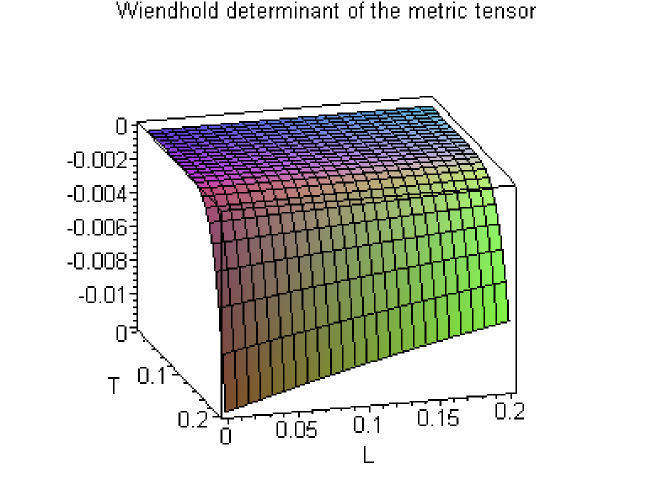
Figure 1: The Wienhold determinant of the metric tensor as a function of temperature, T; and chemical potential, $\lambda=L$ in the $1/2$-BPS supergravity configurations.

We thus see from Fig. 1 that the determinant of the Weinhold metric develops an instability when $T>0.15$. This is also expected, since the coarse graining phenomenon should break down near small effective canonical temperatures. The system is well-defined and physically sound for all $T\in[0,0.15]$.

In order to conclusively analyze the nature of chemical correlations and the concerned properties of the statistical configuration, one needs to determine certain globally invariant quantities on the intrinsic manifold $(M_{2},g)$ of the parameters. In fact, one may easily ascertain that the simplest of such invariants is the scalar curvature of $(M_{2},g)$. In order to do so, one may first compute the Riemann curvature tensor $R_{T\lambda T\lambda}(T,\lambda)$ and then, from the previously defined expression, obtain the scalar curvature. We see that it is not difficult to compute the covariant Riemann tensor $R_{T\lambda T\lambda}(T,\lambda)$. The exact expression for the $R_{T\lambda T\lambda}(T,\lambda)$ is quite involved and thus we relegate it to the Appendix B.

In a straightforward fashion we can show, by applying our previously advertised intrinsic geometric technology, that one may easily obtain the scalar curvature simply via the relation

$$R(T,\lambda)=\frac{R_{T\lambda T\lambda}(T,\lambda)}{||g(T,\lambda)||}$$ (45)

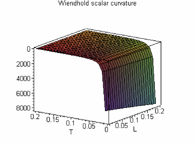
Figure 2: The Wienhold scalar curvature as a function of temperature, T; and chemical potential, $\lambda=L$ in the $1/2$-BPS supergravity configurations.

We observe from Fig. 2 that the system becomes strongly correlated for $T<0.05$, and for $T\in[0.01,0.02]$ it acquires the chemical correlation length of $8\times 10^{3}$. Interestingly, we do not see any chemical fluctuations for $T>0.08$. In the domain of small chemical potentials $T,\lambda\in[0,0.2]$, the pictorial views of the stability may be perceived from the determinant of the Weinhold metric tensor $g^{(E)}(T,\lambda)$ and the concerned correlation length from the corresponding scalar curvature $R^{(E)}(T,\lambda)$. We notice that both the plot of the determinant and that of the scalar curvature of the Wienhold geometry are nice regular 3D hyper-surfaces.

We thence realize that the microcanonical representation of the black holes under consideration posits that there exists a large number of correlated degenerate microscopic states of the $1/2$ BPS giants and superstars. The non-vanishing scalar curvature suggests that a constituent microstate may as well avoid that the initial pure states collapses to a particular pure black hole microstate. This is because of the fact that the intrinsic geometric structures of AdS black hole can be deduced by certain suitably defined subtle measurements [1], and thus there is no loss of information.

5 The Fluctuating Young Tableaux

As in the previous section, the present section is devoted to investigate the notion of large number of boxes into our state-space geometry, and thereby we shall analyze the possible role of concerned large integers in the veritable giant black hole configurations, being considered in the framework of liquid droplet model or fuzzball description. In this concern, we shall precisely compute the statistical pair correlations under this consideration, which ascribes a set of self convincing physical meaning to the state-space quantities, for the simplest excited giant configurations

$$S(n,M)=ln((M^{2})!)-ln(n!)-ln((M^{2}-n)!)$$ (46)

Employing the previously proclaimed formulation, one may easily read off the components of the covariant state-space metric tensor to be

$$g_{nn}(n,M)=\Psi(1,n+1)+\Psi(1,M^{2}-n+1)$$ (47)

$$g_{nM}(n,M)=-2M\Psi(1,M^{2}-n+1)$$ (48)

$$g_{MM}(n,M)=4M^{2}\Psi(1,M^{2}-n+1)-4M^{2}\Psi(1,M^{2}+1)-2\Psi(M^{2}+1)+2\Psi(M^{2}-n+1)$$ (49)

In the above expressions, the $\Psi(n,x)$ is the $n^{th}$ polygamma function, which is the $n^{th}$ derivative of the usual digamma function. Specifically, it turns out that the $\Psi(x)$ may defined to be

$$\Psi(x)=\frac{\partial}{\partial x}\ln(\Gamma(x))$$ (50)

In this framework, we observe that there exists a very simple description which divulges the geometric nature of the statistical pair correlations. The fluctuating extremal black holes may thus easily be determined in terms of the mass and angular momentum of the underlying configurations. Moreover, it is evident that the principle components of the statistical pair correlations are positive definite, for a range of the parameters of the concerned black holes, which physically signifies a certain self-interaction of a fictitious particle moving on an intrinsic surface $(M_{2}(R),g)$. Significantly, it is clear in this case that the following state-space metric constraints hold:

$$g_{nn} > 0,\ \ \forall\ (n,M)\ |\ \Psi(1,n+1)+\Psi(1,M^{2}-n+1)>0$$ (51)

$$g_{MM} > 0,\ \ \forall\ (n,M)\ |\ \Psi(1,M^{2}-n+1)-\Psi(1,M^{2}+1)>$$

$$\frac{1}{2M^{2}}(\Psi(M^{2}+1)-\Psi(M^{2}-n+1))$$

Consequently, we may easily reveal that the common domain of the above state-space constraints defines the range of physically sensible values of the chosen number of boxes and total number of boxes, such that the giants may remain into certain locally stable statistical configurations. We may also notice that the total boxes component $g_{MM}$ of the state-space metric tensor is asymmetrical, in comparison to the $g_{nM}$ and $g_{nn}$. This is physically well-accepted, because of the fact that the component associated with the large number of boxes is somewhat like the heavy head-on collision of two equal particles, which alternate more energy, in contrast to the other excitations, either involving the single particle or the excited-unexcited particles. It is pertinent to mention that the relative pair correlation function determines the selection parameter for a chosen black hole, which may be defined as the modulus of the ratio of excited-excited to excited-unexcited statistical correlations. Importantly, we procure that the parameter thus apprised may be given as the ratio of two digamma functions

$$a:=\frac{1}{2M}|\frac{\Psi(1,n+1)}{\Psi(1,M^{2}-n+1)}|$$ (52)

It is worth to mention that when $n>1$, one has $\Psi(n,x)=\Psi(n)+\gamma$, which is an ordinary rational number, where the $\gamma$ is the standard Euler’s constant. For small values of $n$, $\Psi(n)$ is computed as a sum of gamma functions, which is again a rational number. To force this computation to be performed for larger values of the $n$, we may use

$$\Psi(n,x)=\frac{\partial^{n}\Psi(x)}{\partial x^{n}},$$ (53)

with $\Psi(0,x)=\Psi(x)$. Moreover, the stability of the underlying statistical configurations may earnestly be analyzed by computing the degeneracy of the associated two dimensional state-space manifold. In fact, we may easily ascertain that the determinant of the state-space metric tensor may be given to be

$$g(n,M) = -4M^{2}\Psi(1,n+1)\Psi(1,M^{2}+1)-2\Psi(1,n+1)\Psi(M^{2}+1)$$

$$+4M^{2}\Psi(1,n+1)\Psi(1,M^{2}-n+1)+2\Psi(1,n+1)\Psi(M^{2}-n+1)$$

$$-4M^{2}\Psi(1,M^{2}-n+1)\Psi(1,M^{2}+1)-2\Psi(1,M^{2}-n+1)\Psi(M^{2}+1)$$

$$+2\Psi(1,M^{2}-n+1)\Psi(M^{2}-n+1)$$

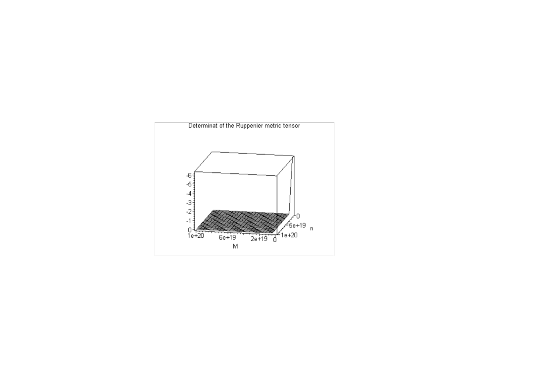
Figure 3: The Ruppenier determinant of the state-space metric tensor as a function of excited droplets, $n$; and total number of fundamental cells, $M^{2}$ in the $1/2$-BPS supergravity configurations.

Fig. 3 indicates that the canonical configurations become unstable and ill-defined when both of the $n$ and $M$ take small values. Up to $10^{5}$ boxes, we discover that the same qualitative features hold. Particularly, it is worth to mention that the fluctuation bumps are aligned towards the $n^{th}$ boundary, when $n$ and $M$ are of the same order.

The determinant of the metric tensor thus calculated is non-zero for any set of given non-zero total boxes and excited boxes, and thus, for the set of proper choices, it provides a non-degenerate state-space geometry for this configuration. In turn, one may illustrate the order of statistical correlations between the equilibrium microstates of the giant black hole system. Besides the fact that the principle component constraints $\{g_{ii}>\ 0\ |\ i=n,M\}$ imply that this system may accomplish certain locally stable statistical configurations, however the negativity of the determinant of the state-space metric tensor indicates that the underlying systems may globally endure a certain instability, as well for the bad choice of boxes, which correspond to certain unphysical macroscopic configurations.

This significantly connotes that there exists a positive definite volume form on the $(M_{2},g)$, for the good choice of boxes and their excitations. One may thus conclude that this system may remain in the nice chosen configuration or, for certain unacceptable choices, might move to some more stable brane configurations. Furthermore, one may easily examine, in general, that the covariant Riemann correlation tensor may be given by the two large integers characterizing the droplets. However, an explicit expression is given by Eq. (ii) State-space Fluctuations: for the $R_{nMnM}(n,M)$, which is rather involved, and thus we have relegated it to the Appendix B.

Furthermore, in order to examine certain global properties of such black holes phase-space configurations, one is required to determine the associated geometric invariants of the underlying state-space manifold. For the giant and superstar black holes, the simplest invariant turns out to be the state-space scalar curvature, which may easily be computed by using the intrinsic geometric technology defined as the negative Hessian matrix of the entropy captured by the excited contributions. Indeed, we discover that the state-space curvature scalar for the fluctuating giant (and superstar) configurations may easily be depicted. Nevertheless, the exact involved expression for the scalar curvature $R(n,M)$ has been depicted in Eq. (ii) State-space Fluctuations: and is shifted to the Appendix B.

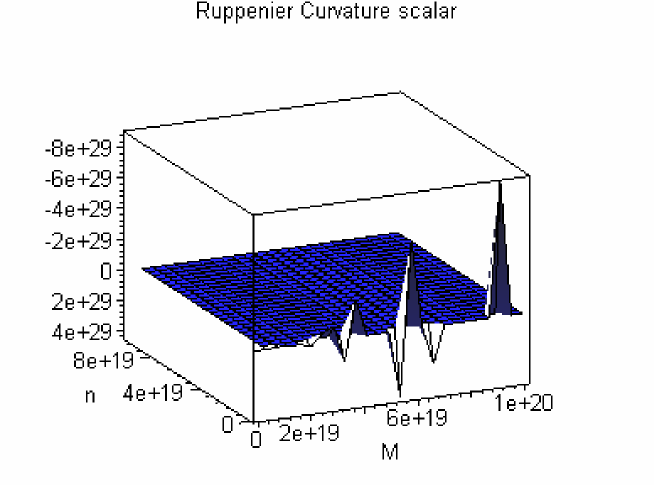
Figure 4: The Ruppenier scalar curvature as a function of excited droplets, $n$, and the total number of fundamental cells, $M^{2}$, in the $1/2$-BPS supergravity configurations.

We numerically find the following conclusions for the state-space scalar curvature correlations.

• For $n,M\in[1,10^{10}]$, it turns out from Fig. 4 that positive, as well as negative correlations exist only along the $M^{th}$ boundary of the state-space configuration. It is also expected from the general consideration of statistical fluctuation theory that the system would possess certain attractions and repulsions.

• We notice, from the respective plots of the determinant and scalar curvature of the state-space configuration, that the system remains stable and regular along the $n^{th}$ boundary of the state-space configuration. We need not mention in this range that the system becomes ill-defined near the origin $(0,0)$ of the state-space manifold.

• We further observe for $10^{4}$ boxes that there exist definite small attraction and repulsion along the $n^{th}$ boundary of the $R$-$n$ surface. Interestingly, the same conclusion remains true for the $g$-$n$ surface of the underlying state-space configuration.

We recognize, in the framework of our state-space geometry, that the negative sign of the curvature scalar signifies that this system is effectively an attractive configuration, under the Gaussian fluctuations. Thus, the giants and superstars appear to be manifestly stable configurations, with nice combinatorial properties of the Young tableaux. Furthermore, we observe that the curvature scalar thus considered is inverse squarely proportional to the determinant of the underlying state-space metric tensor, and thus there are no genuine state-space instability in the underlying microscopic configurations. In turn, we discover that the underlying statistical correlations remain definite, non-zero, finite, regular functions of total boxes and excited boxes carried by the giant black holes.

It is important to note that the state-space geometric quantities may become ill-defined, if the state-space co-ordinates, being defined as the space-time parameters, jump from one existing domain to another domain of the solution. This indicates that the microscopic configurations may correspond to certain interacting statistical systems, in the chosen branch of the full black hole solutions. In an admissible domain of physically acceptable boxes, we discover that the giant black holes have no phase transition, and thus the fundamental statistical configurations are completely free from critical phenomena. Note that the absence of divergences in the scalar curvature indicates that the BPS black brane solutions endure an everywhere thermodynamically stable systems, on their respective state-space configurations.

More generally, we find that the regular state-space scalar curvature seems to be comprehensively universal for the given number of parameters of the configuration. In fact, the concerned idea turns out to be related with the typical form of the state-space geometry, arising from the negative Hessian matrix of the duality invariant expression of the black hole entropy. As in the standard interpretation, the state-space scalar curvature describes the nature of underlying statistical interactions of the possible microscopic configurations, which characteristically turn out to be non-zero, for the $1/2$-BPS black holes. In fact, we may easily appreciate that the constant entropy curve is a standard curve, which may be given by

$$(M^{2})!=c\ n!(M^{2}-n)!$$ (55)

Here, the real constant $c$ can be determined from the given expression of the vacuum entropy. This determines the giant black hole embedding in the view-points of the state-space geometry. Moreover, we may also disclose in the present case that the curve of constant scalar curvature is, however, a complicated curve on the space of total boxes and excited boxes, but the the concerned fundamental nature may easily be fixed by the given number of the boxes. Nonetheless, it is not difficult to enunciate the quantization condition existing on the charges, as we have an integer number of boxes, which in turn signifies a general coordinate transformation in the large number of boxes on the state-space manifold, and may thus be presented in terms of the net number of respective branes.

6 Remarks and Conclusion

This paper provides an exact intrinsic thermodynamic geometric account of the canonical energy fluctuations and box counting entropy for the giants and superstars. The arguments required have been accomplished from an ensemble of Young tableaux with certain randomly excited boxes, while the remaining boxes were kept intact. We notice that the microcanonical representations of the black holes under consideration posit a large number of correlated degenerate microscopic states. These microstates may be evaded by showing that an initial pure state collapses to a particular pure black hole microstate, whose exact structure can be deduced by suitably subtle measurements [1], along with the loss of information, if any. Here, our focus has been to investigate the implications of correlated states for the $1/2$-BPS supergravity black holes. Our analysis clarifies the nature of underlying equilibrium configurations over the Gaussian fluctuations.

Given the importance of the canonical correlations, we have addressed the following questions: (i) how do the Gaussian correlations of pure microstates look like in the view-points of thermodynamic geometries, (ii) what sorts of correlation areas may distinguish the giants or superstars from each other, and (iii) what is the typical nature of statistical fluctuations over an equilibrium ensemble of CFT microstates? Interestingly, we have explicitly demonstrated that the underlying chemical fluctuations involve ordinary summations, while the state-space fluctuations may simply be depicted by standard polygamma functions. Hereby, we notice that the large black holes in AdS spacetimes, whose horizon sizes are bigger than the scale of the AdS curvature, are stable, and exclusively there is no thermodynamic phase transition. We herewith find a precise matching with the fact that these black holes come into an equilibrium configuration, because the AdS geometries create an effective confining potential [44], and thus yield the stability of the thermodynamic system.

Importantly, our framework exploits the fact that the classical general relativity large black holes come with the basic property that their horizon area satisfies the Bekenstein-Hawking entropy relation. With an understanding of the limiting microscopic configurations, an appropriate intrinsic geometric notion has in effect been offered to the counting problem of the microstates of the giants and superstars. Following the discussion of the Appendix A, this provides an account to the degeneracy of microscopic states in the limit $G_{N}/l_{P}>>1$. The semi-classical approximation thus uncovers that the Boltzmann statistical entropy entails certain well-defined equilibrium microstate systems, upon the inclusion of a quadratic fluctuation on the phase-space configurations. Our analysis thus shows that the $1/2$-BPS giants and superstars are thermodynamically stable objects and do not emit Hawking radiation.

The state-space description shows that a set of exact expressions may easily be given for the quadratic fluctuations, over an equilibrium canonical configuration characterized by possible excited and unexcited droplets, in an ensemble of arbitrary random Young tableaux. In turn, the state-space fluctuations, stability criterion and state-space correlation length have precisely been determined, without any approximation, for a large number of giant gravitons and superstars. Following the standard Riemannian geometric notions, we expose that the chemical configuration yields in general that the chemical pair correlation functions, stability condition and correlation length, for an arbitrary value of the effective canonical temperature and the chemical potential, may be determined over an intrinsic Weinhold manifold. Our intrinsic geometric study, thus, exemplifies that there exists an exact fluctuating statistical configuration, which involves an ensemble of fuzzballs, or a number of liquid droplets.

Furthermore, we can ask how the underlying highly degenerate equilibrium microstates get correlated with the chemical potential, carried by a set of given excited droplets. We have shown, from the perspective of string theory on $AdS_{5}\times S^{5}$, that the five dimensional $R$ charged AdS black holes admit an exact Legendre transformed dual chemical configuration, which may be described in terms of the chemical potential and an effective canonical temperature. Thus, the origin of gravitational thermodynamics comes with the existence of a non-zero thermodynamic curvature, under the coarse graining mechanism of alike “quantum information geometry”, associated with the wave functions of underlying BPS black holes. Notice, further, that the physical meaning of the respective curvatures is that they describe the correlation, in the concerned ensemble of black holes. Characteristically, it is worth to mention that the semi-classical gravitational description, arising with the non-vanishing scalar curvature, signifies the existence of the throat of the underlying AdS background.

We notice an intriguing support, from the Mathur’s fuzzball proposal, that the leading order entropy should come from those fuzzs, whose radius varies as the fuzzy throat of the black hole horizon size. Furthermore, the liquid droplet model suggests that the AdS length scales like $L\sim l_{P}f(N_{i})$, where $N_{i}$ is the number of bound states [1, 2]. It has further been suggested that the classical description is achieved, when $N\rightarrow\infty$ while $\hbar\rightarrow 0$, such that the Fermi level $N/\hbar$ remains constant. Most importantly, we have investigated the role of thermodynamic fluctuations in the two parameter giants and superstars, whose chemical and state-space configurations are being respectively characterized by the chemical variables of the effective canonical ensemble, and by the number of both excited and total boxes, constituting an ensemble of arbitrary shaped CFT microstates. The present analysis thus explicates that the underlying chemical and state-space configurations are well-defined, non-degenerate and regular, for all physically admissible domains of the statistical parameters, defining an ensemble of arbitrary fuzzballs, or a set of indiscriminate liquid droplets.

Now, we enlist a number of attributes arising from our study of the thermodynamic intrinsic geometry of (dual) giants and superstars, divulged in the framework of liquid droplets or fuzzball solutions. The intriguing nature of the chemical and the state-space correlations, existing in an underlying statistical basis, ascribes that the local and global thermodynamic structures, thus revealed, may in either case be summarized as follows.

6.1 Chemical Description:

Following our specific notions, we exclusively observe that the chemical configurations of the $1/2$ BPS giants and superstars realize the following general properties:

• There exists an exact expression for the chemical pair correlation functions, stability condition and correlation length, for arbitrary values of $T,\lambda\in M_{2}$.

• Explicit plots displayed in the Figs. 1 and 2 show that the determinant and scalar curvature are non-trivially curved, and surprisingly the results remain the same, even for a single component with $j=1$.

• We further reveal, from the numerical conclusions displayed in Figs. 1 and 2, that the Weinhold metric tensor, and the corresponding correlation length, show that the statements of stability and regularity hold for all $\lambda\in M_{2}$.

6.2 State-space Description:

In this case, the findings obtained from the intrinsic state-space geometry from an ensemble of Young tableaux may be summarized as

• A set of exact precise expressions may easily be given for the state-space fluctuations, over an equilibrium canonical ensemble, characterized by possible arbitrary random Young tableaux.

• The state-space fluctuations, stability criterion and state-space correlation length may easily be determined without any approximation.

• We can express the $g^{(S)}_{ij}(n,M)$, $g^{(S)}(n,M)$ and $R^{(S)}(n,M)$ in terms of nice, well-behaved digamma $\Psi(n)$ and poly-gamma $\Psi(n,M)$ functions. Notice that the mixing between excited and non-excited droplets or fuzzs may precisely be caused by these standard polygamma functions.

• The concerned state-space geometry corresponds to a non-degenerate, locally stable and attractive statistical configuration.

• The underlying numerical computations plotted in Figs. 3 and 4 disclose that the state-space correlation exists along the boundary of $n$ and $M$, for non-large $n$, $M$, when we take approximately $1$ to $10^{5}$ boxes in the Young diagrams.

It is worth to mention that the present analysis takes into account the scales, that are larger than the respective correlation length, and contemplates that just a few giant or superstar microstates cannot dominate the entire macroscopic solution. Most importantly, we have procured that the thermodynamic intrinsic geometric structures of the canonical energy and box counting entropy provide a coherent framework, to further study the thermodynamic geometries, arising from the large number of microstates of the chosen giants, superstars and the other superconformal field theory and supergravity configurations [46].

Finally, it is worth to mention that the interpretation of a non-zero intrinsic scalar curvature, with an underlying interacting statistical system, remains valid even for higher dimensional intrinsic Riemannian manifolds. The implication of a divergent intrinsic covariant curvature may accordingly be divulged, from the Hessian matrix of the canonical energy or the box counting entropy, irrespectively whether, or not, there exists a phase transition in the $1/2$ BPS black hole configurations.

Appendix A

In this appendix, we provide precise expression for the case of two parameter thermodynamic configuration. This review set-up is offered from the viewpoint of two parameter family giant and superstar solutions. In order to do so, we recall important recent studies of the thermodynamic properties of diverse (rotating) black holes have elucidated interesting aspects of phase transitions, if any, in the state-space geometric framework and their associated relations with the extremal black hole solutions in the context of $\mathcal{N}\geq 2$ compactifications [24, 25]. It may be argued however that the connection of such a geometric formulation to the thermodynamic fluctuation theory of black holes requires several modifications [26]. The geometric formulation thus involved has first been applied to $\mathcal{N}\geq 2$ supergravity extremal black holes in $D=4$, which arise as low energy effective field theories from the compactifications of Type II string theories on Calabi-Yau manifolds [27]. Since then, several authors have attempted to understand this connection [28, 29, 30, 31], for both the supersymmetric as well as non-supersymmetric four dimensional black holes and five dimensional rotating black string and ring solutions. Interesting discussions on the vacuum phase transitions, if any, exist in the literature, which involves some change of the black hole horizon topology, [28, 29, 30, 31].

Ruppenier has conjointly advocated the assumption “that all the statistical degrees of freedom of black hole live on the black hole event horizon”, and thus the scalar curvature signifies the average number of correlated Planck areas on the event horizon of the black hole [33]. Specifically, the zero scalar curvature indicates certain bits of information on the event horizon fluctuating independently of each other, while the diverging scalar curvature signals a phase transition indicating highly correlated pixels of the informations. Moreover, Bekenstein has introduced an elegant picture for the quantization of the area of the event horizon, being defined in terms of Planck areas [34]. Recently, the state-space geometry of the equilibrium configurations thus described has extensively been applied to study the thermodynamics of a class of rotating black hole configurations [21, 35, 36, 37].

From the viewpoint of the present consideration, the underlying moduli configuration appears to be horizonless and smooth. However, in the classical limit in which the Planck length and the AdS throat scale as, respectively $l_{P}\rightarrow 0$ and $L\rightarrow 0$, in such a way that their ratio diverges $l_{P}/L\rightarrow\infty$, the underlying moduli configuration acquires an entropy which may be assumed to be associated with the average horizon area of the black hole. In general, one wishes to compare the quantization of a classical moduli space from the known perspective of the AdS/CFT correspondence [5, 6]. In this concern, it is worth to mention that we have

$$AdS/CFT:\ \{\mathcal{N}=4\ SYM\}\ \leftrightarrow\ \{Type\ IIB\ String\ Theory\ on\ AdS_{5}\times S^{5}\}$$ (56)

Following [1, 2], it is important to mention that the supergravity description emerges in the strong coupling limit with $g^{2}_{YM}N>>$ 1while, the dual CFT emerges in the weak coupling limit $g^{2}_{YM}N<<1$. Thus, one finds the matching of entropies in the $\frac{1}{2}$ BPS sector of the configuration [1, 2]. In this sector, the authors of [1, 2] have shown that nearly all states look alike and they belong to the same chiral ring quantization of the classical moduli space. It is however intriguing to note that the dual CFT formalism faces problems with the wave functional renormalization, mixing of states, and in general it may feature certain other technical difficulties as well [1, 2]. Nevertheless, none of these concerns the present analysis, and thus we may safely divulge the probable fluctuations over chosen equilibrium giants configurations.

As mentioned in the introduction, the $1/2$-BPS (dual) giant configurations are parameterized by two chemical potentials, $\lambda_{1},\lambda_{2}$. Thus, the fluctuations around the minima energy configuration are describe an intrinsic Wienhold surface. Explicitly, let us consider the case of the two dimensional intrinsic chemical geometry, such that the components of the metric tensor are given by

$$g_{\lambda_{1}\lambda_{1}} = \frac{\partial^{2}E}{\partial\lambda_{1}^{2}}$$

$$g_{\lambda_{1}\lambda_{2}} = \frac{\partial^{2}E}{{\partial\lambda_{1}}{\partial\lambda_{2}}}$$

$$g_{\lambda_{2}\lambda_{2}} = \frac{\partial^{2}E}{\partial\lambda_{2}^{2}}$$ (57)

In this case, it follows that the determinant of the metric tensor is

$$\|g(\lambda_{1},\lambda_{2})\| = S_{\lambda_{1}\lambda_{1}}S_{\lambda_{2}\lambda_{2}}-S_{\lambda_{1}\lambda_{2}}^{2}$$ (58)

Now, we can calculate the $\Gamma_{ijk}$, $R_{ijkl}$, $R_{ij}$ and $R$ for the above two dimensional thermodynamic geometry $(M_{2},g)$. One may easily inspect that the scalar curvature is given by

$$R(\lambda_{1},\lambda_{2}) = -\frac{1}{2}(E_{\lambda_{1}\lambda_{1}}E_{\lambda_{2}\lambda_{2}}-E_{\lambda_{1}\lambda_{2}}^{2})^{-2}(E_{\lambda_{2}\lambda_{2}}E_{\lambda_{1}\lambda_{1}\lambda_{1}}E_{\lambda_{1}\lambda_{2}\lambda_{2}}$$ (59)

$$+E_{\lambda_{1}\lambda_{2}}E_{\lambda_{1}\lambda_{1}\lambda_{2}}E_{\lambda_{1}\lambda_{2}\lambda_{2}}+E_{\lambda_{1}\lambda_{1}}E_{\lambda_{1}\lambda_{1}\lambda_{2}}E_{\lambda_{2}\lambda_{2}\lambda_{2}}$$

$$-E_{\lambda_{1}\lambda_{2}}E_{\lambda_{1}\lambda_{1}\lambda_{1}}E_{\lambda_{2}\lambda_{2}\lambda_{2}}-E_{\lambda_{1}\lambda_{1}}E_{\lambda_{1}\lambda_{2}\lambda_{2}}^{2}-E_{\lambda_{2}\lambda_{2}}E_{\lambda_{1}\lambda_{1}\lambda_{2}}^{2})$$

Furthermore, the relation between the chemical scalar curvature and the Riemann covariant curvature tensor for any two dimensional intrinsic geometry is given (see for details [21]) by

$$R=\frac{2}{\|g\|}R_{\lambda_{1}\lambda_{2}\lambda_{1}\lambda_{2}}$$ (60)

The relation Eq. 60 is quite usual for an arbitrary intrinsic Riemannian surface $(M_{2}(R),g)$. Correspondingly, the Legendre transformed version of the Wienhold manifold is known as state-space manifold. In fact, the associated configuration is parameterized by the number of excited and total boxes, i.e. $\{n,M\}$. Thus, the Gaussian fluctuation of the entropy of $1/2$-BPS configurations form a two dimensional state-space surface $M_{2}$. Explicitly, the components of covariant state-space metric tensor may be given as

$$g_{nn} = -\frac{\partial^{2}S(n,M)}{\partial n^{2}}$$

$$g_{nM} = -\frac{\partial^{2}S(n,M)}{{\partial n}{\partial M}}$$

$$g_{MM} = -\frac{\partial^{2}S(n,M)}{\partial M^{2}}$$ (61)

It is easy to express, in this simplest case, that the determinant of the metric tensor turns out to be

$$\|g(n,M)\| = S_{nn}S_{MM}-S_{nM}^{2}$$ (62)

As in the case of Wienhold geometry, we find that the state-space scalar curvature is given by

$$R(n,M) = \frac{1}{2}(S_{nn}S_{MM}-S_{nM}^{2})^{-2}(S_{MM}S_{nnn}S_{nMM}+S_{nM}S_{nnM}S_{nMM}$$ (63)

$$+ S_{nn}S_{nnM}S_{MMM}-S_{nM}S_{nnn}S_{MMM}-S_{nn}S_{nMM}^{2}-S_{MM}S_{nnM}^{2})$$

Following the observations of [35], it is essentially evident that the scalar curvature and the corresponding Riemann curvature tensor of an arbitrary two dimensional intrinsic state-space manifold $(M_{2}(R),g)$ may be given by

$$R(n,M)=\frac{2}{\|g\|}R_{nMnM}(n,M)$$ (64)

Appendix B

In this appendix, we provide the explicit form of the most general thermodynamic scalar curvatures describing the family of two charged giant and superstars. Our analysis illustrates that the physical properties of the specific scalar curvatures may exactly be exploited, without any approximation. The definite behavior of curvatures, as accounted in section three, suggests that the various intriguing chemical and state-space examples of $1/2$ BPS solutions include the nice property that they do not diverge, except for the determinant singularity. As mentioned in the main sections, these configurations are an interacting statistical system. We discover that their thermodynamic geometries indicate the possible nature of general two parameter equilibrium configurations. Significantly, one may notice, from the very definition of intrinsic metric tensors, that the relevant Riemann covariant curvature tensors and scalar curvatures may be thus presented as follows.

(i) Canonical Energy Fluctuations:

Here, we shall explicitly supply the exact Riemann covariant tensor of the Weinhold geometry for the 2- parameter giants and superstars. It turns out that the functional nature of a large number of gravitons, within the neighborhood of small chemical fluctuations introduced in the canonical ensemble of $1/2$ BPS configurations, may precisely be divulged. Surprisingly, we expose in this framework, that the intrinsic covariant curvature tensor takes the exact and simple expression

$$R_{T\lambda T\lambda}(T,\lambda) = -\frac{1}{4}\{(\sum_{j=0}^{\infty}(-j^{2}\frac{b_{j}}{T^{4}}\frac{(-2T+2Tb_{j}+j+jb_{j})}{(b_{j}-1)^{3}}))\times(\sum_{j=0}^{\infty}(-jb_{j}\frac{(1+b_{j})}{(b_{j}-1)^{3}})$$

$$-(\sum_{j=0}^{\infty}(j^{2}\frac{b_{j}}{T^{2}}\frac{(1+b_{j})}{(b_{j}-1)^{3}}))^{2}\}^{-1}\{-(\sum_{j=0}^{\infty}(-jb_{j}\frac{(1+b_{j})}{(b_{j}-1)^{3}}))\times$$

$$(\sum_{j=0}^{\infty}(-j^{2}\frac{b_{j}}{T^{4}}\frac{(-2T+2Tb_{j}^{2}+j+4jb_{j}+jb_{j}^{2})}{(b_{j}-1)^{4}}))^{2}+(\sum_{j=0}^{\infty}(-jb_{j}\frac{(1+b_{j})}{(b_{j}-1)^{3}}))\times$$

$$(\sum_{j=0}^{\infty}(j^{2}\frac{b_{j}}{T^{6}}\frac{(j^{2}+4j^{2}b_{j}+j^{2}b_{j}^{2}-6jT+6T^{2}+6jTb_{j}^{2}-12T^{2}b_{j}+6T^{2}b_{j}^{2})}{(b_{j}-1)^{4}}))$$

$$\times(\sum_{j=0}^{\infty}(j^{2}\frac{b_{j}}{T^{2}}\frac{(1+4b_{j}+b_{j}^{2})}{(b_{j}-1)^{4}}))+(\sum_{j=0}^{\infty}(j^{2}\frac{b_{j}}{T^{2}}\frac{(1+b_{j})}{(b_{j}-1)^{3}}))\times$$

$$(\sum_{j=0}^{\infty}(-j^{2}\frac{b_{j}}{T^{4}}\frac{(-2T+2Tb_{j}^{2}+j+4jb_{j}+jb_{j}^{2})}{(b_{j}-1)^{4}}))\times$$

$$(\sum_{j=0}^{\infty}(j^{2}\frac{b_{j}}{T^{2}}\frac{(1+4b_{j}+b_{j}^{2})}{(b_{j}-1)^{4}}))-(\sum_{j=0}^{\infty}(j^{2}\frac{b_{j}}{T^{2}}\frac{(1+b_{j})}{(b_{j}-1)^{3}}))\times$$

$$(\sum_{j=0}^{\infty}(j^{2}\frac{b_{j}}{T^{6}}\frac{(j^{2}+4j^{2}b_{j}+j^{2}b_{j}^{2}-6jT+6T^{2}+6jTb_{j}^{2}-12T^{2}b_{j}+6T^{2}b_{j}^{2})}{(b_{j}-1)^{4}}))$$

$$\times(\sum_{j=0}^{\infty}(-jb_{j}\frac{(1+4b_{j}+b_{j}^{2})}{(b_{j}-1)^{4}}))-(\sum_{j=0}^{\infty}(-j^{2}\frac{b_{j}}{T^{4}}\frac{(-2T+2Tb_{j}+j+jb_{j})}{(b_{j}-1)^{3}}))\times$$

$$(\sum_{j=0}^{\infty}(j^{2}\frac{b_{j}}{T^{2}}\frac{(1+4b_{j}+b_{j}^{2})}{(b_{j}-1)^{4}}))^{2}+(\sum_{j=0}^{\infty}(-j^{2}\frac{b_{j}}{T^{4}}\frac{(-2T+2Tb_{j}+j+jb_{j})}{(b_{j}-1)^{3}}))\times$$

$$(\sum_{j=0}^{\infty}(-j^{2}\frac{b_{j}}{T^{4}}\frac{(-2T+2Tb_{j}^{2}+j+4jb_{j}+jb_{j}^{2})}{(b_{j}-1)^{4}}))\times(\sum_{j=0}^{\infty}(-jb_{j}\frac{(1+4b_{j}+b_{j}^{2})}{(b_{j}-1)^{4}}))\}$$

(ii) State-space Fluctuations:

As stated earlier, the state-space metric in the excited and unexcited droplets is given by the negative Hessian matrix of the box counting entropy. Here, the numbers of excited and empty boxes in a given Young diagram are respected to be extensive variables. In this case, the two distinct large integers characterize the intrinsic state-space correlation length, carried by the giants and superstars. Our computation shows that the exact Riemann covariant curvature tensor is given by

$$R_{nMnM}(n,M) = 1/2\{(-2M^{2}\Psi(1,n+1)\Psi(1,M^{2}+1)-\Psi(1,n+1)\Psi(M^{2}+1)$$

$$+2M^{2}\Psi(1,n+1)\Psi(1,M^{2}-n+1)+\Psi(1,n+1)\Psi(M^{2}-n+1)$$

$$-2M^{2}\Psi(1,M^{2}-n+1)\Psi(1,M^{2}+1)-\Psi(1,M^{2}-n+1)\Psi(M^{2}+1)$$

$$+\Psi(1,M^{2}-n+1)\Psi(M^{2}-n+1))\}^{-1}[\Psi(1,n+1)\Psi(1,M^{2}-n+1)^{2}$$

$$-\Psi(1,M^{2}-n+1)\Psi(2,n+1)\Psi(M^{2}+1)$$

$$+\Psi(1,M^{2}-n+1)\Psi(2,n+1)\Psi(M^{2}-n+1)$$

$$+\Psi(2,M^{2}-n+1)\Psi(1,M^{2}-n+1)\Psi(M^{2}+1)$$

$$-\Psi(2,M^{2}-n+1)\Psi(1,M^{2}-n+1)\Psi(M^{2}-n+1)$$

$$+2M^{2}\{3\Psi(2,M^{2}-n+1)\Psi(1,n+1)\Psi(1,M^{2}+1)$$

$$+2\Psi(1,M^{2}-n+1)\Psi(2,n+1)\Psi(1,M^{2}+1)$$

$$-2\Psi(1,M^{2}-n+1)^{2}\Psi(2,n+1)+\Psi(1,M^{2}-n+1)^{3}$$

$$-\Psi(2,M^{2}-n+1)\Psi(2,n+1)\Psi(M^{2}+1)$$

$$+\Psi(2,M^{2}-n+1)\Psi(2,n+1)\Psi(M^{2}-n+1)$$

$$-\Psi(2,M^{2}-n+1)\Psi(1,n+1)\Psi(1,M^{2}-n+1)$$

$$+\Psi(2,M^{2}-n+1)\Psi(1,M^{2}-n+1)\Psi(1,M^{2}+1)\}$$

$$+4M^{4}\{\Psi(2,M^{2}-n+1)\Psi(1,n+1)\Psi(2,M^{2}+1)$$

$$-\Psi(2,M^{2}-n+1)\Psi(2,n+1)\Psi(1,M^{2}+1)$$

$$+\Psi(1,M^{2}-n+1)\Psi(2,n+1)\Psi(2,M^{2}+1)\}]$$

Finally, let us turn our attention to the state-space scalar curvature for the two parameter droplet configurations. A systematic examination demonstrates that the scalar curvature is

$$R(n,M) = \frac{1}{2}\{-2\Psi(1,n+1)\Psi(1,M^{2}+1)M^{2}-\Psi(1,n+1)\Psi(M^{2}+1)$$

$$+2M^{2}\Psi(1,n+1)\Psi(1,M^{2}-n+1)+\Psi(1,n+1)\Psi(M^{2}-n+1)$$

$$-2M^{2}\Psi(1,M^{2}-n+1)\Psi(1,M^{2}+1)-\Psi(1,M^{2}-n+1)\Psi(M^{2}+1)$$

$$+\Psi(1,M^{2}-n+1)\Psi(M^{2}-n+1)\}^{-2}$$

$$[\Psi(1,M^{2}-n+1)^{3}+\Psi(1,n+1)\Psi(1,M^{2}-n+1)^{2}$$

$$-\Psi(1,M^{2}-n+1)\Psi(2,n+1)\Psi(M^{2}+1)$$

$$+\Psi(1,M^{2}-n+1)\Psi(2,n+1)\Psi(M^{2}-n+1)$$

$$+\Psi(2,M^{2}-n+1)\Psi(1,M^{2}-n+1)\Psi(M^{2}+1)$$

$$-\Psi(2,M^{2}-n+1)\Psi(1,M^{2}-n+1)\Psi(M^{2}-n+1)$$

$$+2M^{2}\{\Psi(2,M^{2}-n+1)\Psi(1,M^{2}-n+1)\Psi(1,M^{2}+1)$$

$$-\Psi(2,M^{2}-n+1)\Psi(1,n+1)\Psi(1,M^{2}-n+1)$$

$$-\Psi(2,M^{2}-n+1)\Psi(2,n+1)\Psi(M^{2}+1)$$

$$+\Psi(2,M^{2}-n+1)\Psi(2,n+1)\Psi(M^{2}-n+1)$$

$$-2\Psi(1,M^{2}-n+1)^{2}\Psi(2,n+1)$$

$$+2\Psi(1,M^{2}-n+1)\Psi(2,n+1)\Psi(1,M^{2}+1)$$

$$+3\Psi(2,M^{2}-n+1)\Psi(1,n+1)\Psi(1,M^{2}+1)\}$$

$$+4M^{4}\{\Psi(2,M^{2}-n+1)\Psi(1,n+1)\Psi(2,M^{2}+1)$$

$$+\Psi(1,M^{2}-n+1)\Psi(2,n+1)\Psi(2,M^{2}+1)$$

$$-\Psi(2,M^{2}-n+1)\Psi(2,n+1)\Psi(1,M^{2}+1)\}]$$

References

- [1] V. Balasubramanian, J. de Boer, V. Jejjala, J. Simon, “The Library of Babel: On the origin of gravitational thermodynamics”, JHEP 0512 (2005) 006, arXiv:hep-th/0508023v2.
- [2] V. Balasubramanian, M. Berkooz, A. Naqvi, M. J. Strassler, “Giant gravitons in conformal field theory”, JHEP 0204, 034 (2002), arXiv:hep-th/0107119.
- [3] V. Balasubramanian, J. de Boer, V. Jejjala, J. Simon, “Entropy of near-extremal black holes in ”, JHEP 0805, 067 (2008), arXiv:0707.3601v2 [hep-th].
- [4] K. Huang, “Statistical Mechanics”, John Wiley, 1963, L. D. Landau, E. M. Lifshitz, “Statistical Physics-I, II”, Pergamon, 1969.
- [5] H. Lin, O. Lunin, and J. Maldacena, “Bubbling AdS space and 1/2 BPS geometries”, JHEP 0410, 025 (2004).
- [6] S. Bellucci, E. Ivanov, S. Krivonos, “AdS/CFT Equivalence Transformation”, Phys. Rev. D 66, 086001 (2002); Erratum-ibid. D 67, 049901 (2003), arXiv:hep-th/0206126.
- [7] S. Bellucci, A. Galajinsky, E. Ivanov, S. Krivonos, “, Canonical Transformations and Superconformal Mechanics”, Phys. Lett. B 555, 99-106 (2003); arXiv:hep-th/0212204.
- [8] O. Lunin, S. D. Mathur, “Metric of the multiply wound rotating string”, Nucl. Phys. B 610, 49 (2001), arXiv:hep-th/0105136.
- [9] S. S. Gubser, J. J. Heckman, “Thermodynamics of R-charged Black Holes in AdS(5) From Effective Strings”, JHEP 0411, 052 (2004), arXiv:hep-th/0411001v2.
- [10] S. D. Mathur, “Where are the states of a black hole”, OHSTPY-HEP-T-04-001, arXiv:hep-th/0401115.
- [11] S. D. Mathur, A. Saxena, Y. K. Srivastava, “Constructing ’hair’ for the three charge hole”, arXiv:hep-th/0311092.
- [12] J. Simon, “Small Black holes vs horizonless solutions in AdS”, Phys. Rev. D 81, 024003 (2010), arXiv:0910.3225v2 [hep-th].
- [13] F. Weinhold, “Metric geometry of equilibrium thermodynamics”, J. Chem. Phys. 63 , 2479 (1975), DOI:10. 1063/ 1. 431689.
- [14] F. Weinhold, “Metric geometry of equilibrium thermodynamics. II”, Scaling, homogeneity, and generalized Gibbs–Duhem relations, ibid J. Chem. Phys 63 , 2484 ( 1975).
- [15] G. Ruppeiner, “Riemannian geometry in thermodynamic fluctuation theory”, Rev. Mod. Phys 67 (1995) 605, Erratum 68 (1996) 313.
- [16] M. Santoro, A. S. Benight, “On the geometrical thermodynamics of chemical reactions”, math-ph/0507026.
- [17] G. Ruppeiner, “Thermodynamics: A Riemannian geometric model”, Phys. Rev. A 20, 1608 (1979).
- [18] G. Ruppeiner, “Thermodynamic Critical Fluctuation Theory?”, Phys. Rev. Lett. 50, 287 (1983).
- [19] G. Ruppeiner, “New thermodynamic fluctuation theory using path integrals”, Phys. Rev. A 27,1116,1983.
- [20] G. Ruppeiner and C. Davis, “Thermodynamic curvature of the multicomponent ideal gas”, Phys. Rev. A 41, 2200, 1990.
- [21] B. N. Tiwari, “Sur les corrections de la géométrie thermodynamique des trous noirs”, arXiv:0801.4087v1 [hep-th].
- [22] T. Sarkar, G. Sengupta, B. N. Tiwari, “Thermodynamic Geometry and Extremal Black Holes in String Theory”, JHEP 0810, 076, 2008, arXiv:0806.3513v1 [hep-th].
- [23] T. Sarkar, G. Sengupta, B. N. Tiwari, “On the Thermodynamic Geometry of BTZ Black Holes”, JHEP 0611 (2006) 015, arXiv:hep-th/0606084v1.
- [24] S. Bellucci, S. Ferrara, A. Marrani, “Attractor Horizon Geometries of Extremal Black Holes”, Contribution to the Proceedings 27 of the XVII SIGRAV Conference, 4-7 September 2006, Turin, Italy, arXiv:hep-th/0702019.
- [25] S. Bellucci, S. Ferrara, A. Marrani, “Attractors in Black”, Contribution to the Proceedings of the 3rd RTN Workshop Constituents, Fundamental Forces and Symmetries of the Universe, 1-5 October 2007, Valencia, Spain, Fortsch. Phys. 56 (2008) 761, arXiv:0805.1310.
- [26] G. Ruppeiner, “Thermodynamic curvature and phase transitions in Kerr-Newman black holes”, Phys. Rev. D 75, 024037 (2007).
- [27] S. Ferrara, G. W. Gibbons, R. Kallosh, “Black Holes and Critical Points in Moduli Space”, Nucl. Phys. B500, 75 (1997) hep-th/9702103.
- [28] J. Shen, R. G. Cai, B. Wang, R. K. Su, “Thermodynamic Geometry and Critical Behavior of Black Holes”, Int. J. Mod. Phys. A 22 (2007) 11-27, arXiv:gr-qc/0512035v1.
- [29] J. E. Aman, I. Bengtsson, N. Pidokrajt, “Geometry of black hole thermodynamics”, Gen. Rel. Grav. 35 (2003) 1733, arXiv:gr-qc/0304015v1.
- [30] J. E. Aman, N. Pidokrajt, “Geometry of Higher-Dimensional Black Hole Thermodynamics”, Phys. Rev. D 73 (2006) 024017, arXiv:hep-th/0510139v3.
- [31] G. Arcioni and E. Lozano-Tellechea, “Stability and critical phenomena of black holes and black rings”, Phys. Rev. D 72, 104021 (2005).
- [32] S. D. Mathur, “The fuzzball proposal for black holes: An elementary review”, Fortsch. Phys. 53 (2005) 793, arXiv:hep-th/0502050.
- [33] G. Ruppeiner, “Thermodynamic curvature and phase transitions in Kerr-Newman black holes”, Phy. Rev. D 78, 024016 (2008).
- [34] D. Bekenstein, “Information in the holographic universe”, Sci. Am. 289, No. 2, 58-65 (2003).
- [35] S. Bellucci, B. N. Tiwari, “On the Microscopic Perspective of Black Branes Thermodynamic Geometry”, arXiv:0808.3921v1 [hep-th].
- [36] S. Bellucci, B. N. Tiwari, “State-space Manifold and Rotating Black Holes”, To appear.
- [37] S. Bellucci, B. N. Tiwari, “Black Strings, Black Rings and State-space Manifold”, To appear.
- [38] O. Lunin, S. D. Mathur, “AdS/CFT Duality and the Black Hole Information Paradox”, Nucl. Phys. B 623 (2002) 342, arXiv:hep-th/0109154.
- [39] V. Balasubramanian, F. Larsen, “On D-Branes and Black Holes in Four Dimensions”, Nucl. Phys. B 478, 199 (1996), arXiv:hep-th/9604189.
- [40] S. Corley, A. Jevicki, and S. Ramgoolam, “Exact correlators of giant gravitons from dual N = 4 SYM theory”, Adv. Theor. Math. Phys. 5, 809 (2002) arXiv:hep-th/0111222.
- [41] D. Berenstein, “A toy model for the AdS/CFT correspondence”, JHEP 0407, 018 (2004), arXiv:hep-th/0403110.
- [42] R. C. Myers, and O. Tafjord, Superstars and “giant gravitons”, JHEP 0111, 009 (2001) arXiv:hep-th/0109127.
- [43] N. V. Suryanarayana, “Half-BPS giants, free fermions and microstates of superstars”, JHEP 0601, 082, 2006, arXiv:hep-th/0411145.
- [44] S. W. Hawking and D. N. Page, Thermodynamics of Black “Holes In Anti-De Sitter Space”, Commun. Math. Phys. 87, 577 (1983).
- [45] E. G. Gimon, F. Larsen, J. Simon, “Black Holes in Supergravity: the non-BPS Branch”, JHEP 0801, 040 (2008), arXiv:0710.4967v3 [hep-th].
- [46] J. M. Maldacena, “The Large N Limit of Superconformal Field Theories and Supergravity”, Adv. Theor. Math. Phys. 2 (1998) 231-252; arXiv:hep-th/9711200v3.