An alternative well-posedness property and static spacetimes with naked singularities

Abstract

In the first part of this paper, we show that the Cauchy problem for wave propagation in some static spacetimes presenting a singular time-like boundary is well posed, if we only require the waves to have finite energy, although no boundary condition is required. This feature does not come from essential self-adjointness, which is false in these cases, but from a different phenomenon that we call the alternative well-posedness property, whose origin is due to the degeneracy of the metric components near the boundary.

Beyond these examples, in the second part, we characterize the type of degeneracy which leads to this phenomenon.

1 Introduction

The aim of this paper is to investigate the well-posedness of the Cauchy problem for the propagation of waves in static spacetimes presenting a singular time-like boundary, and to clarify the boundary behaviour of the waves. Such singularities can arise when solving Einstein equations in the vacuum or in situations where matter is present but located away from singularities.

This line of research has been initiated by Wald in [1], and further developed by, among others, the authors of references [2, 3, 4, 5, 6].

The propagation of waves is formally given by a standard wave equation of the form

$$\partial_{tt}\phi+A\phi=0,$$

where $A$ is a second-order symmetric operator with variable coefficients independent of time, defined on $C^{\infty}_{0}(\Omega)$, the space of test functions (see 2.1 for precise definitions). Hence, the Cauchy problem is well-posed as soon as one is able to choose a physically meaningful self-adjoint extension of $A$, on the Hilbert space $H$ naturally associated to the setting.

In most cases, this is done either by adding suitable boundary conditions or because $A$ turns out to be essentially self-adjoint. Since here, there is no physically meaningful boundary condition, many authors discussed the essentially self-adjointness of $A$: although never explicitely proved, the above cited papers are based on the fact that $A$ does not fulfill this property.

This is the reason why, in [3], the authors suggested to replace $H$ by another space, on which they claimed that one recovers the essentially self-adjointness of $A$. However, this is wrong, and we prove it at the end of the first part.

Other choices have been to deal with the Friedrichs extension of $A$, the most clear argument for doing so being stated in [6]: “the Friedrichs extension is the only one whose domain is contained in $H^{1}$”. In this work we show how this observation turns out to be at the core of the problem:

When no boundary conditions can be provided (physically or mathematically), by choosing the Friedrichs extension, the solution turns out naturally to have finite energy. But, of course, this extension cannot be interpreted as imposing any boundary condition.

On the other hand, requiring the solutions the condition to have finite energy is, in general, not enough to have a well posed problem. However, it may occur, that under this sole condition, the problem turns out to be well-posed without any boundary condition, i.e., the solution is completely determined by the Cauchy data. Indeed, as we show in this work, it happens when the smallest possible space (the completion of smooth compactly supported functions on $\Omega$ with the energy norm) coincides with the largest possible one: the energy space (which obviously contains functions that do not vanish at the boundary).

In part I, we show this for explicit examples: Taub’s plane symmetric spacetime [7] and its generalization to higher dimensions [8], and Schwarzschild solution with negative mass. The last one has already been discussed in the literature [2, 3].

The singularity of spacetime induces non standard behavior of the coefficients of $A$ when the point reaches the boundary. Roughly speaking, in the normal direction to the boundary, the coefficients vanish, while they explode in the parallel direction. In particular, the normal coefficient vanishes like some power of the distance to the boundary.

We start by showing that the operator $A$ is not essentially self-adjoint. Hence, we have to choose one of its many self-adjoint extensions. Our criterion is to require the waves to have finite energy at any time.

Contrary to the standard cases (like, for instance, vibrating strings), where boundary conditions are needed, we show here that this sole condition is enough to select a unique self-adjoint extension of $A$. No boundary conditions must be imposed to functions in the domain of this extension, and the Cauchy problem is well-posed with initial conditions only.

However, the absence of boundary condition does not imply the absence of boundary behaviour. As a matter of fact, it happens that the waves do have a non trivial boundary behaviour, i.e., a trace on $\partial\Omega$, which moreover obeys a regularity law which depends on the above mentioned exponent.

In the second part, we turn our attention to the general problem of deciding when boundary conditions are needed or not for the Cauchy problem to be well-posed in the absence of essential self-adjointness. Our setting is that for a divergence operator on the half-space, fulfilling a pointwise ellipticity condition; we do not prescribe any a priori form of global ellipticity, thus allowing arbitrary degeneracies near the boundary (provided the coefficients remain locally integrable up to the boundary, however). Paralleling somehow our first part, we use the Dirichlet form associated to the operator to define an energy space which is the largest possible space whose elements all have finite energy. Then, we say that the operator has the alternative well-posedness property if it has one and only one self-adjoint extension with domain included in the energy space.

We clarify the link between this property and the density in the energy space of test functions compactly supported in the geometric domain. On the basis of this abstract preliminary, we finally give a necessary condition and a sufficient condition for this property to hold. Under a mild assumption on the coefficients of the operators, which is reminiscent of Muckenhoupt $A_{2}$ class, these conditions are equivalent, so that we obtain a characterization of the alternative well-posedness property. Its application to static spacetimes such as the examples above is straightforward.

Part I. Wave propagation in Taub’s spacetime and other examples

2 Massless scalar field in Taub’s plane symmetric spacetime

2.1 Geometric setting

We consider the $(n+2)$-dimensional spacetime with $n\geq 2$ and line element

$$ds^{2}=-z^{-1+\frac{1}{n}}\,\left(dt^{2}-dz^{2}\right)+z^{2/n}\left[(dx^{\scriptscriptstyle 1})^{2}+\dots+(dx^{\scriptscriptstyle{n}})^{2}\right],$$

$$-\infty<t<\infty,\quad\quad-\infty<x^{\scriptscriptstyle{i}}<\infty,\,1\leq i\leq n,\quad\quad 0<z<\infty\,.$$

Throughout the paper, we will use the following notation: in $\Omega=\mathbb{R}^{n}\times(0,\infty)$, the current point is $(x,z)$, with $x=(x^{\scriptscriptstyle{1}},...,x^{\scriptscriptstyle{n}})\in\mathbb{R}^{n}$, $z>0$; the Lebesgue measure on $\Omega$ is $d\mu$, and on $\mathbb{R}^{n}$ is $dx$; the gradient and the Laplacian on $\mathbb{R}^{n}$ are $\nabla=(\partial_{x^{\scriptscriptstyle{1}}},...,\partial_{x^{\scriptscriptstyle{n}}})^{T}$ and $\Delta=\sum_{i=1}^{n}\partial_{x^{\scriptscriptstyle{i}}x^{\scriptscriptstyle{i}}}$.

When $n=2$, this spacetime is Taub’s plane symmetric vacuum solution [7], which is the unique nontrivial static and plane symmetric solution of Einstein vacuum equations ($R_{ab}=0$). It has a singular boundary at $z=0$ (see [9] for a detailed study of the properties of this solution).

By matching it to inner solutions it turns out to be the exterior solution of some static and plane symmetric distributions of matter [9, 10, 11]. In such a case, the singularities are not the sources of the fields, but they arise owing to the attraction of distant matter. We call them empty repelling singular boundaries (see also [12]).

In this spacetime, we consider the propagation of a massless scalar field with Lagrangian density

$$\mathscr{L}=-\frac{1}{2}\nabla^{a}\phi\,\nabla_{a}\phi=-\frac{1}{2}g^{ab}\partial_{a}\phi\,\partial_{b}\phi\ ,$$ (1)

where $\nabla$ denotes the covariant derivative (Levi-Civita connection).

As usual, we obtain the field equations by requiring that the action

$$S=\int\mathscr{L}(\nabla_{a}\phi,\phi,g_{ab})\sqrt{|g|}\ dtd\mu\$$

be stationary under arbitrary variations of the fields $\delta\phi$ in the interior of any compact region, but vanishing at its boundary. Thus, we have

$$\nabla_{a}\left(\frac{\partial\mathscr{L}}{\partial\ \!\nabla_{a}\phi}\ \right)=\frac{\partial\mathscr{L}}{\partial\ \!\phi}\ .$$

In our case, this reads

$$\nabla_{a}\nabla^{a}\phi\ = \frac{\partial_{a}\left(\sqrt{|g|}\,g^{ab}\partial_{b}\phi\right)}{\sqrt{|g|}}$$ (2)

$$= z^{-1+\frac{1}{n}}\left(-\,\partial_{tt}\phi+{\frac{1}{z}\partial_{z}(z\,\partial_{z}\phi)}+\frac{1}{z^{1+\frac{1}{n}}}\Delta\phi\right)$$

$$= 0.$$

As it is well known (see for example [13]), from the Lagrangian density $\mathscr{L}$ we get the energy-stress tensor

$$T^{ab}=-\frac{\partial\mathscr{L}}{\partial\ \!\nabla_{a}\phi}\ \nabla^{b}\phi\ +g^{ab}\mathscr{L}=g^{ac}g^{bd}\,\partial_{c}\phi\,\partial_{d}\phi-\frac{1}{2}g^{ab}g^{cd}\,\partial_{c}\phi\,\partial_{d}\phi\ ,$$

which is symmetric and, for smooth enough solution of (2), has vanishing covariant divergence ($\nabla_{a}T^{ab}=0$). Since the spacetime is stationary, $\partial_{t}$ is a Killing vector field. Therefore by integrating $(-(\partial_{t})_{b}T^{bt})$ over the whole space we get that, whenever it exists, the total energy of the field configuration is

$$E(\phi,t)=\frac{1}{2}\int_{\Omega}\left(z\,(\partial_{t}\phi)^{2}+z\,(\partial_{z}\phi)^{2}+\frac{1}{z^{\frac{1}{n}}}\,(\nabla\phi)^{2}\right)\,dx\,dz.$$

2.2 Statement of the results

To study the properties of the solutions of the wave equation (2), we start with defining the underlying elliptic differential operator $A$ and the Hilbert space $H$ on which $A$ is symmetric.

Define, when $\varphi\in C_{0}^{\infty}(\Omega)$, the operator $A$ by

$$A\varphi=-\frac{1}{z}\partial_{z}\left(z\,\partial_{z}\varphi\right)-\frac{1}{z^{1+\frac{1}{n}}}\Delta\varphi.$$

Then consider the Hilbert space

$$H := L^{2}(\Omega,z\,d\mu)$$

$$= \{\varphi(x,z)\ :\ \int_{\Omega}|\varphi(x,z)|^{2}\,z\,d\mu<\infty\}.$$

By construction the operator $A$ is symmetric on $H$, with

$$<A\varphi,\eta>_{H} = \int_{\Omega}\left(z\partial_{z}\varphi\,\partial_{z}\bar{\eta}\,+\frac{1}{z^{\frac{1}{n}}}\nabla\varphi\cdot\nabla\bar{\eta}\right)d\mu$$

$$= :b(\varphi,\eta)$$

for $\varphi,\eta\in C_{0}^{\infty}(\Omega)$.

This leads to introducing the “energy space”

$$\mathcal{E}=\{\varphi\in H^{1}_{loc}(\Omega)\cap H\ :\,b(\varphi,\varphi)<\infty\},$$ (3)

where $H^{1}_{loc}(\Omega)$ is the usual local Sobolev space. It is straightforward to check that $\mathcal{E}$, equipped with its natural norm

$$\|\varphi\|^{2}_{\mathcal{E}}:=b(\varphi,\varphi)+\|\varphi\|^{2}_{H},$$

is a Hilbert space. This is the largest subspace of $H$ on which the form $b$ is finite everywhere.

Remark 2.1

The space $C_{c}^{\infty}(\Omega)$ of the restrictions to $\Omega$ of $C_{0}^{\infty}(\mathbb{R}^{n+1})$ functions is included in $\mathcal{E}$; to prove that it is dense in both $H$ and $\mathcal{E}$ is left to the reader.

Our first question is whether $A$ is essentially self-adjoint or not: as a result, it is not. However, we are only looking for those extensions with domain included in the energy space, because we are interested in waves having finite energy. When taking into account this restriction, we recover the uniqueness of the self-adjoint extension of $A$.

Theorem 2.2

The operator $A$ is not essentially self-adjoint. However, there exists only one self-adjoint extension of $A$ whose domain $D$ is included in the energy space $\mathcal{E}$.

We will see later that the domain of this particular extension is

$$D:=\{\varphi\in\mathcal{E}\ :\exists\ C>0\ \forall\ \eta\in\mathcal{E},\ |b(\varphi,\eta)|\leq C\|\eta\|_{H}\}.$$

Notation 2.3

For the sake of simplicity, the self-adjoint extension of $A$ given by the theorem above is denoted the same way.

In the next section we will show that the uniqueness of such an extension comes from the density in $\mathcal{E}$ of $C_{0}^{\infty}(\Omega)$. This important density property prevents the space $\mathcal{E}$ to possess any kind of trace operator or, more generally, any continuous linear form supported on the boundary. Hence there is no boundary condition attached to the definition of $A$.

Now, coming back to the wave equation, we take suitable functions $f$ and $g$ on $\Omega$ and consider the Cauchy problem  

$$(P)\left\{\begin{array}[]{cc}\partial_{tt}\phi+A\phi&=0,\\ \phi(0,\cdot)&=f,\\ \partial_{t}\phi(0,\cdot)&=g.\end{array}\right.$$

Theorem 2.4

1. Assume $f\in\mathcal{E}$ and $g\in H$. Then the problem (P) has a unique solution

   $$\phi\in C([0,\infty);\mathcal{E})\cap C^{1}([0,\infty);H),$$

   and there exists a constant $C>0$ such that

   $$\forall\ t>0\ \ \ \|\phi(t,\cdot)\|_{\mathcal{E}}+\|\partial_{t}\phi(t,\cdot)\|_{H}\leq C(\|f\|_{\mathcal{E}}+\|g\|_{H}).$$

2. In this case, the energy

   $$E(\phi,t):=\frac{1}{2}\int_{\Omega}\left(z\,(\partial_{t}\phi)^{2}+z\,(\partial_{z}\phi)^{2}+\frac{1}{z^{\frac{1}{n}}}\,|\nabla\phi|^{2}\right)d\mu$$

   is well-defined and conserved:

   $$\forall\ t>0\ \ \ E(\phi,t)=\frac{1}{2}\left(\|g\|_{H}^{2}+b(f,f)\right).$$

3. If, in addition, $f\in D$ and $g\in\mathcal{E}$, we have

   $$\phi\in C([0,\infty);D)\cap C^{1}([0,\infty);\mathcal{E}),$$

   and, for another constant $C>0$,

   $$\forall\ t>0\ \ \ \|\phi(t,\cdot)\|_{D}+\|\partial_{t}\phi(t,\cdot)\|_{\mathcal{E}}\leq C(\|f\|_{D}+\|g\|_{\mathcal{E}}).$$

This result shows that the Cauchy problem (P) is well posed without any boundary condition on $\phi$. This does not necessarily mean, however, that $\phi(t,\cdot)$ vanishes, or has no trace at all, on the boundary. Indeed, provided $f$ and $g$ are regular enough, $\phi(t,\cdot)$ does have a trace on $\partial\Omega$ at each time $t>0$, which is entirely determined by the Cauchy data:

Theorem 2.5

Assume $f\in D$ and $g\in\mathcal{E}$, and let $\phi$ be the solution of (P) given by Theorem 2.4. Then, for each $t>0$, ${\displaystyle\lim_{z\to 0}\phi(t,\cdot,z)}$ exists in $L^{2}(\mathbb{R}^{n})$.

By standard arguments, at each fixed $z>0$, the trace $\phi(t,\cdot,z)$ on the hyperplane $\Gamma_{z}=:\{(x,z);x\in\mathbb{R}^{n}\}$ exists in the Sobolev space ${H}^{1}(\mathbb{R}^{n})$ (even in ${H}^{3/2}(\mathbb{R}^{n})$, see for instance [14]). This theorem says that the trace of $\phi$ on the boundary exists as the strong limit of $\phi(t,\cdot,z)$, for the $L^{2}$-topology, of its traces on $\Gamma_{z}$ when $z\rightarrow 0$.

We could have written down the theorem above with stronger topologies, namely that of ${H}^{1}$ and even ${H}^{3/2}$. But there exists a more striking result. If we denote by $\phi(t,\cdot,0)$ the trace of $\phi(t,\cdot)$ on $\partial\Omega$, we have

Theorem 2.6

Under the preceding hypotheses, $\phi(t,\cdot,0)\in{H}^{\frac{2n}{n-1}}(\mathbb{R}^{n})$ for each $t>0$, and we have more precisely $\phi(\cdot,\cdot,0)\in C([0,\infty);{H}^{\frac{2n}{n-1}}(\mathbb{R}^{n}))$.

If it was a classical case, the trace of $\phi(t)$ would be at most in ${H}^{3/2}(\mathbb{R}^{n})$ because $\phi(t)$ would be in ${H}^{2}(\Omega)$. This is what happens for $\phi(t,\cdot,z)$ at each $z>0$, which has no reason to be in ${H}^{\frac{2n}{n-1}}(\mathbb{R}^{n})$ unless additional assumptions on $\phi$ are made. What happens here is a compensation phenomenon between the normal and the tangential degeneracies of the coefficients of $A$ near the boundary, so that there is a gain of regularity on the trace $\phi(t,\cdot,0)$ with respect to the regularity of $\phi(t,\cdot,z)$, $z>0$.

The theorems stated above will be deduced from the results of the following section.

3 The domain of $A$ and its properties

3.1 The space $\mathcal{E}$ and the definition of $A$

Lemma 3.1

$C_{0}^{\infty}(\Omega)$ is dense in $\mathcal{E}$.

We pointed out in section 2 that $C_{c}^{\infty}(\Omega)$ is included and dense in $\mathcal{E}$. This Lemma, hence, implies that there is no trace operator in $\mathcal{E}$ . Let us be more precise. We claim that there exists no topological linear space $F$ and no operator $T$ such that  
i) $T$ is linear and continuous from $\mathcal{E}$ to $F$.  
ii) If $\varphi\in C_{c}^{\infty}(\Omega)$, then $\varphi(\cdot,0)\in F$, and $T\varphi=\varphi(\cdot,0)$.

Indeed, property ii) implies that $T$ vanishes on $C_{0}^{\infty}(\Omega)$ but not on $\mathcal{E}$, which contradicts i) and Lemma 3.1.

Let us now prove the Lemma. It suffices to approximate in $\mathcal{E}$ any $\varphi\in C_{c}^{\infty}(\Omega)$ by functions in $C_{0}^{\infty}(\Omega)$. Let $\varphi\in C_{c}^{\infty}(\Omega)$. We first construct $\varphi_{\varepsilon}\in C_{c}(\Omega)\cap\mathcal{E}$ for all $\varepsilon>0$ such that $\varphi_{\varepsilon}(x,0)=0$ and $\displaystyle{\lim_{\varepsilon\to 0}\varphi_{\varepsilon}=\varphi\ \mbox{ in}\ \mathcal{E}}$. To this purpose, we set

$$\varphi_{\varepsilon}(x,z)=\varphi(x,z)h_{\varepsilon}(z),$$

where

$$h_{\varepsilon}(z)=\left\{\begin{array}[]{cc}\frac{1}{\varepsilon}|\log z|^{-\varepsilon}&\ \mbox{if}\ \ z\leq z(\varepsilon)\\ 1&\ \mbox{if}\ \ z>z(\varepsilon),\end{array}\right.$$

with $\displaystyle{|\log z(\varepsilon)|=\varepsilon^{-\frac{1}{\varepsilon}}}$; then $\varphi_{\varepsilon}(x,z)\in C_{c}(\Omega)\cap\mathcal{E}$ for all $\varepsilon>0$. Furthermore, notice that

$$\int_{0}^{\infty}|\partial_{z}h_{\varepsilon}|^{2}z\,dz=\int_{z\leq z(\varepsilon)}|\log z|^{-2-2\varepsilon}\;\frac{1}{z}\;dz\underset{\varepsilon\to 0}{\longrightarrow}0.$$

Using this observation and the dominated convergence theorem, it is straightforward to obtain

$$\|\varphi_{\varepsilon}-\varphi\|_{\mathcal{E}}\underset{\varepsilon\to 0}{\longrightarrow}0.$$ (4)

Then, for all $\varepsilon>0,\alpha>0$, we define

$$\varphi_{\varepsilon,\alpha}(\cdot,z)=\left\{\begin{array}[]{cc}\varphi_{\varepsilon}(\cdot,z-\alpha)&\ \mbox{if}\ z\geq\alpha,\\ 0&\ \mbox{if}\ z\leq\alpha.\end{array}\right.$$

Since $\varphi_{\varepsilon}$ vanishes on $\partial\Omega$, we have

$$\varphi_{\varepsilon,\alpha}\underset{\alpha\to 0^{+}}{\longrightarrow}\varphi_{\varepsilon}.$$

With (4) and the fact that $\varphi_{\varepsilon,\alpha}\in C_{0}(\Omega)\cap\mathcal{E}$, this gives the density in $\mathcal{E}$ of $C_{0}(\Omega)\cap\mathcal{E}$. The proof of the lemma finishes with a standard regularization scheme.

$\Box$

We define the operator $\mathcal{A}$ on the domain

$$D=\{\varphi\in\mathcal{E}\ :\,\exists\ C>0\ \forall\ \eta\in\mathcal{E},\ |b(\varphi,\eta)|\leq C\|\eta\|_{H}\}$$

by the classical procedure: if $\varphi\in D$, there exists $\psi\in H$ such that $\displaystyle{b(\varphi,\eta)=<\psi\,,\eta>}$ for all $\eta\in\mathcal{E}$, and we set $\psi=\mathcal{A}\varphi$.

Proof of Theorem 2.2:

By the symmetry of the bilinear form $b(\varphi,\eta)$ and by the definition of $D$, $(\mathcal{A},D)$ is a self-adjoint extension of $(A,C_{0}^{\infty}(\Omega))$. Now by Lemma 3.1, $(\mathcal{A},D)$ is the Friedrichs extension of $(A,C_{0}^{\infty}(\Omega))$; thus it is the only extension with domain included in $\mathcal{E}$.

In order to see that $(A,C_{0}^{\infty}(\Omega))$ is not essentially self-adjoint it is enough to give a function $\eta$ such that $\eta\in D(A^{*})$, where

$$D(A^{*})=\{\eta\in H\ :\,\exists\ C>0:\forall\varphi\in C_{0}^{\infty}(\Omega),\ |<\eta,A\varphi>|\leq C\|\varphi\|_{H}\},$$

and $\eta\notin\mathcal{E}$.

Taking $\eta$ such that its Fourier transform in $x$ is $\hat{\eta}(\xi,z)=K_{0}(\frac{2n}{n-1}\ z^{\frac{n-1}{2n}}|\xi|)$, where $K_{0}$ is the modified Bessel function of the second kind, we have that $\eta\in H,\ A^{*}\eta=0$, and $\eta\notin\mathcal{E}$ (the properties of the function $\eta$ are discussed below, see Remark 3.3), thus the proof is finished.

$\Box$

As already mentioned, from now on we do not distinguish between both operators, and use the letter $A$ to denote them.

Remark 3.2

Let $\psi$ in $H$. Then, if we consider the equation $\psi=A\varphi$, where $\varphi\in H$, in the distribution sense, either it has a unique solution or it has no solution. Prescribing some boundary condition would lead to an overdetermined problem, with no solution in general.

3.2 Traces of functions in $D$

Our second key result is that although there is no trace operator in the whole space $\mathcal{E}$, every function in the domain $D$ does have a trace on $\partial\Omega$. If $\varphi\in D$ we denote by $\varphi(z)$ its trace on the subspace $\Gamma_{z}=\mathbb{R}^{n}\times\{z\}$, $z>0$. Such a trace exists thanks to classical results on elliptic operators with $C^{\infty}$ coefficients, [14].

In order to study the behavior of $\varphi(z)$ in $L^{2}(\mathbb{R}^{n})$, we consider $\psi\in H$ such that $A\varphi=\psi$. Taking the Fourier Transform in $x$, we write this equation as

$$\hat{A\varphi}(\xi,z)=-\frac{1}{z}\;\partial_{z}\big{(}z\,\partial_{z}\hat{\varphi}(\xi,z)\big{)}+\frac{|\xi|^{2}}{z^{1+\frac{1}{n}}}\hat{\varphi}(\xi,z)\,=\hat{\psi}(\xi,z).$$ (5)

Any solution of the differential equation

$$z\,u^{\prime\prime}(z)+u^{\prime}(z)-\frac{1}{z^{\frac{1}{n}}}u(z)\,=-z\,v(z)$$ (6)

can be written as

$$u(z)=\left(\int_{z}^{\infty}s\,v(s)\,u_{1}(s)\,ds+C_{0}\right)\,u_{0}(z)+\left(\int_{0}^{z}s\,v(s)\,u_{0}(s)\,ds+C_{1}\right)\,u_{1}(z),$$

with $u_{0}(z)=I_{0}\left(\frac{z^{\alpha_{n}}}{\alpha_{n}}\right)$ and $u_{1}(z)=\frac{1}{\alpha_{n}}K_{0}\left(\frac{z^{\alpha_{n}}}{\alpha_{n}}\right)$, where $\alpha_{n}=\frac{1}{2}-\frac{1}{2n}$ and $I_{0}$ and $K_{0}$ are modified Bessel functions and solutions of the homogeneous ordinary differential equation associated with (6).

Remark 3.3

Near the origin, the behavior of the solutions $u_{0}(z)$ and $u_{1}(z)$ is:

$$\hskip-42.67912ptu_{0}(z)=1+\frac{z^{{1}-\frac{1}{n}}}{(1-\frac{1}{n})^{2}}\,+O\left(z^{{2}-\frac{2}{n}}\right),\;\;u_{0}^{\prime}(z)=\frac{z^{-\frac{1}{n}}}{(1-\frac{1}{n})}\,+O\left(z^{{1}-\frac{2}{n}}\right),$$

$$u_{1}(z)=-\log(z)+c+O\left(z^{{1}-\frac{1}{n}}\right),u_{1}^{\prime}(z)=-\frac{1}{z}+c\ {z^{-\frac{1}{n}}}+O\left(\log(z)z^{-\frac{1}{n}}\right),$$

where $c$ is a different constant in each equation.

Also, for large values of $z$, we have

$$u_{0}(z) = \left({\sqrt{\frac{\alpha_{n}}{2\pi}}}\,\,z^{-\frac{\alpha_{n}}{2}}+O\left(z^{-\frac{3\alpha_{n}}{2}}\right)\right)e^{\frac{z^{\alpha_{n}}}{\alpha_{n}}}$$

$$u_{0}^{\prime}(z) = \left({\sqrt{\frac{\alpha_{n}}{2\pi}}}\,\,z^{-1+\frac{\alpha_{n}}{2}}+O\left(z^{-1-\frac{\alpha_{n}}{2}}\right)\right)e^{\frac{z^{\alpha_{n}}}{\alpha_{n}}}$$

$$u_{1}(z) = \left(\sqrt{\frac{\pi}{2\,\alpha_{n}}}\,z^{-\frac{\alpha_{n}}{2}}+O\left(z^{-\frac{3\alpha_{n}}{2}}\right)\right)e^{-\frac{z^{\alpha_{n}}}{\alpha_{n}}}$$

$$u_{1}^{\prime}(z) = -\left(\sqrt{\frac{\pi}{2\,\alpha_{n}}}\,z^{-1+\frac{\alpha_{n}}{2}}+O\left(z^{-1-\frac{\alpha_{n}}{2}}\right)\right)e^{-\frac{z^{\alpha_{n}}}{\alpha_{n}}}.$$

As a consequence of this remark we obtain that for $\psi\in L^{2}((0,\infty),z\,dz)$, the only solution $u$ to (6) such that $u$ and $\partial_{z}u$ belong to $L^{2}((0,\infty),z\,dz)$ is

$$u(z)=\left(\int_{z}^{\infty}s\,v(s)\,u_{1}(s)\,ds\right)\,u_{0}(z)+\left(\int_{0}^{z}s\,v(s)\,u_{0}(s)\,ds\right)\,u_{1}(z).$$

By scaling in the equation (6), we obtain that the only solution to (5) which belongs to $\hat{\mathcal{E}}=:\{\hat{\varphi}:\varphi\in\mathcal{E}\}$ is

$$\hat{\varphi}(\xi,z) = \left(\int_{z}^{\infty}s\,\hat{\psi}(\xi,s)\,u_{1}(s|\xi|^{\frac{1}{\alpha_{n}}})\,ds\right)\ u_{0}(z|\xi|^{\frac{1}{\alpha_{n}}})$$ (7)

$$+ \left(\int_{0}^{z}s\,\hat{\psi}(\xi,s)\,u_{0}(s|\xi|^{\frac{1}{\alpha_{n}}})\,ds\right)u_{1}(z|\xi|^{\frac{1}{\alpha_{n}}}).$$

Lemma 3.4

Assume $\varphi\in D$ and Supp $\varphi\subset\mathbb{R}^{n}\times[0,1]$. There exists a constant $C$ independent of $\varphi$ such that

$$\sup_{z\leq 1}\|z^{\frac{1}{n}}\,\partial_{z}\varphi(z)\|_{L^{2}(\mathbb{R}^{n})}\leq\,C\|A\varphi\|_{H}.$$

Proof :   By derivating (7) with respect to $z$, we obtain

$$\partial_{z}\hat{\varphi}(\xi,z) = \left(\int_{z}^{\infty}\!\!\!s\,\hat{\psi}(\xi,s)\,u_{1}(s|\xi|^{{\frac{1}{\alpha_{n}}}})ds\right)|\xi|^{{\frac{1}{\alpha_{n}}}}u^{\prime}_{0}(z|\xi|^{{\frac{1}{\alpha_{n}}}})$$ (8)

$$+ \left(\int_{0}^{z}\!\!\!s\,\hat{\psi}(\xi,s)\,u_{0}(s|\xi|^{{\frac{1}{\alpha_{n}}}})ds\right)|\xi|^{{\frac{1}{\alpha_{n}}}}u^{\prime}_{1}(z|\xi|^{{\frac{1}{\alpha_{n}}}}).$$

In order to estimate this function in $L^{2}(\mathbb{R}^{n})$, we fix $z$ and consider first the case $z|\xi|^{\frac{1}{\alpha_{n}}}\geq 1$. We have

$$\left\|\left(\int_{z}^{\infty}\!\!s\,\hat{\psi}(\xi,s)\,u_{1}(s|\xi|^{{\frac{1}{\alpha_{n}}}})ds\right)|\xi|^{{\frac{1}{\alpha_{n}}}}u^{\prime}_{0}(z|\xi|^{{\frac{1}{\alpha_{n}}}})\ \mathbf{1}_{\{z|\xi|^{\frac{1}{\alpha_{n}}}\geq 1\}}\right\|_{L^{2}(d\xi)}^{2}$$

$$\leq\int_{\{z|\xi|^{\frac{1}{\alpha_{n}}}\geq 1\}}\left(\int_{z}^{\infty}s\,|\hat{\psi}(\xi,s)|^{2}ds\right)\left(\int_{z}^{\infty}s\,u^{2}_{1}(s\,|\xi|^{{\frac{1}{\alpha_{n}}}})\,ds\right)|\xi|^{\frac{2}{\alpha_{n}}}u^{\prime 2}_{0}(z|\xi|^{\frac{1}{\alpha_{n}}})\,d\xi.$$

Using the behavior of $u_{1}$ and $u_{0}$ given in the remark 3.3, we obtain

$$\int_{z}^{\infty}s\,u^{2}_{1}(s|\xi|^{\frac{1}{\alpha_{n}}})\,ds\leq Cz^{2-2\alpha_{n}}|\xi|^{-2}e^{-2\frac{z^{\alpha_{n}}}{\alpha_{n}}|\xi|}$$ (9)

and

$$\left\|\left(\int_{z}^{\infty}\!\!s\,\hat{\psi}(\xi,s)\,u_{1}(s|\xi|^{\frac{1}{\alpha_{n}}})ds\right)|\xi|^{\frac{1}{\alpha_{n}}}u^{\prime}_{0}(z|\xi|^{\frac{1}{\alpha_{n}}})\ \mathbf{1}_{\{z|\xi|^{\frac{1}{\alpha_{n}}}\geq 1\}}\right\|_{L^{2}(d\xi)}^{2}\leq C\,\|\psi\|^{2}_{H}.$$

When $z|\xi|^{\frac{1}{\alpha_{n}}}\geq 1$, we also have

$$\int_{0}^{z}s\,u^{2}_{0}(s|\xi|^{\frac{1}{\alpha_{n}}})\,ds\leq Cz^{2-2\alpha_{n}}|\xi|^{-2}e^{2\frac{z^{\alpha_{n}}}{\alpha_{n}}|\xi|}.$$ (11)

This gives

$$\left\|\left(\int_{0}^{z}s\,\hat{\psi}(\xi,s)\,u_{0}(s|\xi|^{\frac{1}{\alpha_{n}}})\,ds\right)|\xi|^{\frac{1}{\alpha_{n}}}u^{\prime}_{1}(z|\xi|^{\frac{1}{\alpha_{n}}})\;\mathbf{1}_{\{z|\xi|^{\frac{1}{\alpha_{n}}}\geq 1\}}\right\|_{L^{2}(d\xi)}^{2}$$

$$\leq\int_{\{z|\xi|^{\frac{1}{\alpha_{n}}}\geq 1\}}\left(\int_{0}^{z}s\,|\hat{\psi}(\xi,s)|^{2}\,ds\right)\left(\int_{0}^{z}s\,u^{2}_{0}(s|\xi|^{\frac{1}{\alpha_{n}}})\,ds\right)|\xi|^{8}u^{\prime 2}_{1}(z|\xi|^{\frac{1}{\alpha_{n}}})\,d\xi$$

$$\leq C\int_{\{z|\xi|^{\frac{1}{\alpha_{n}}}\geq 1\}}\left(\int_{z}^{\infty}s\,|\hat{\psi}(\xi,s)|^{2}\,ds\right)z^{-\alpha_{n}}|\xi|^{-1}d\xi\,\leq C\|\psi\|^{2}_{H}.$$

In the case $z|\xi|^{\frac{1}{\alpha_{n}}}\leq 1$, we use Minkowski inequality and the support condition on $\varphi$ to obtain

$$\left\|\left(\int_{z}^{\infty}s\,\hat{\psi}(\xi,s)\,u_{1}(s|\xi|^{\frac{1}{\alpha_{n}}})\,ds\right)|\xi|^{\frac{1}{\alpha_{n}}}u^{\prime}_{0}(z|\xi|^{\frac{1}{\alpha_{n}}})\ \mathbf{1}_{\{z|\xi|^{\frac{1}{\alpha_{n}}}\leq 1\}}\right\|$$

$$\leq Cz^{-\frac{1}{n}}\int_{z}^{\infty}\sqrt{s}\,\|\hat{\psi}(s)\|_{L^{2}(d\xi)}\,ds\leq Cz^{-\frac{1}{n}}\|\psi\|_{H},$$ (13)

and

$$\left\|\left(\int_{0}^{z}s\,\hat{\psi}(\xi,s)\,u_{0}(s|\xi|^{\frac{1}{\alpha_{n}}})\,ds\right)|\xi|^{\frac{1}{\alpha_{n}}}u^{\prime}_{1}(z|\xi|^{\frac{1}{\alpha_{n}}})\ \mathbf{1}_{\{z|\xi|^{\frac{1}{\alpha_{n}}}\leq 1\}}\right\|_{L^{2}(d\xi)}\,$$

$$\leq C\int_{0}^{z}\frac{s}{z}\,\|\hat{\psi}(\xi,s)\|_{L^{2}(d\xi)}\,ds\leq C\,\|\psi\|_{H}.$$ (14)

Thanks to (3.2), (3.2), (3.2) and (3.2), and recalling that $\psi=A\varphi$, the Lemma is proved.

$\Box$

Let now $\varphi\in D$, and assume first that Supp $\varphi\subset\mathbb{R}^{n}\times[0,1]$. Then the last lemma applies, the formula

$$\varphi(0)=-\int_{0}^{1}\partial_{z}\varphi(z)dz$$

defines the trace $\varphi(0)$ of $\varphi$ on $\partial\Omega$, and gives that $\varphi(0)\in L^{2}(\mathbb{R}^{n})$, with

$$\|\varphi(0)\|_{L^{2}(\mathbb{R}^{n})}\leq C\|A\varphi\|_{H}.$$ (15)

In the general case, where $\varphi$ does not satisfy any support condition, we modify $\varphi$ in $\tilde{\varphi}$ by setting

$$\tilde{\varphi}(x,z)=\varphi(x,z)h(z),$$

where $h\in C^{\infty}(\mathbb{R})$ is such that $h(z)=1$ when $z\leq\frac{1}{2}$ and $h(z)=0$ when $z\geq 1$. It is easy to check that $\tilde{\varphi}\in D$ and that

$$\|A\tilde{\varphi}\|_{H}\leq\|A\varphi\|_{H}+C\|\varphi\|_{\mathcal{E}}.$$

The inequality (15) applied to $\tilde{\varphi}$, with the fact that $\tilde{\varphi}=\varphi$ on $\mathbb{R}^{n}\times[0,\frac{1}{2}]$, ends the proof of Theorem 2.5, giving the estimate

$$\|\varphi(0)\|_{L^{2}(\mathbb{R}^{n})}\leq C\left(\|A\varphi\|_{H}+\|\varphi\|_{\mathcal{E}}\right).$$ (16)

The additional regularity of the trace is contained in the next more precise result:

Lemma 3.5

Let $\varphi\in D$ and $\psi\in H$ such that $A\varphi=\psi$. Then

$$\hskip-42.67912pti)\ \ \sup_{z\leq\frac{1}{2}}\|z^{\frac{1}{n}}\,\partial_{z}\varphi(z)\|_{L^{2}(\mathbb{R}^{n})}\leq\,C\left(\|A\varphi\|_{H}+\|\varphi\|_{\mathcal{E}}\right),$$ (17)

$$\hskip-42.67912ptii)\ \ \Delta\varphi(0)\in L^{2}(\mathbb{R}^{n})\ \ and\ \ \|\Delta\varphi(0)\|_{L^{2}(\mathbb{R}^{n})}\leq C\left(\|A\varphi\|_{H}+\|\varphi\|_{\mathcal{E}}\right),$$ (18)

$$\hskip-42.67912ptiii)\ \ \Delta\varphi(0)=-\lim_{z\to 0}(1-\frac{1}{n})z^{\frac{1}{n}}\,\partial_{z}\varphi(z)\ \ {in\ the\ strong\ topology\ of\ }L^{2}(\mathbb{R}^{n}).$$ (19)

$$\hskip-42.67912ptiv)\ \ \Delta^{\frac{n}{n-1}}\varphi(0)\in L^{2}(\mathbb{R}^{n}).$$ (20)

v) Moreover, the preceding statement is sharp, in the sense that for any
$\gamma\in H^{\frac{2n}{n-1}}(\mathbb{R}^{n})$, there exist $\varphi\in D$ such that $\varphi(0)=\gamma$.

Proof :   The proof of i) goes through replacing $\varphi$ with $\tilde{\varphi}$ and applying Lemma 3.4, as we did for deducing (16) from (15).

We continue the proof using the same trick, and in order to alleviate the notation, we write $\varphi$ instead of $\tilde{\varphi}$. The second step of the proof consists in showing that

$$\lim_{z\to 0}(1-\frac{1}{n})z^{\frac{1}{n}}\,\partial_{z}\varphi(z)=\lambda(z),$$ (21)

where $\lambda$ is defined by

$$\hat{\lambda}(\xi)=|\xi|^{2}\int_{0}^{\infty}\!\!s\,\hat{\psi}(\xi,s)\,u_{1}(s|\xi|^{\frac{1}{\alpha_{n}}})ds,$$

and the limit is taken in the strong $L^{2}$-topology.

To prove that $\lambda\in L^{2}(\mathbb{R}^{n})$ is straightforward: since $z\mapsto z^{2\alpha_{n}}\ u_{1}(z)$ is bounded, we have by the support condition on $\varphi$ that

$$|\hat{\lambda}(\xi)|\leq\int_{0}^{1}\!\!s^{1-2\alpha_{n}}\,|\hat{\psi}(\xi,s)|\,ds,$$ (22)

which implies

$$\|\lambda\|_{L^{2}(\mathbb{R}^{n})}\leq C\|\psi\|_{H},$$ (23)

by Cauchy Schwarz inequality.

Now, by Remark 3.3, $u^{\prime}_{0}(z)\sim\frac{z^{-\frac{1}{n}}}{(1-\frac{1}{n})}\,+O\left(z^{{1}-\frac{2}{n}}\right)$ when $z\to 0$. Using this in the proof of Lemma 3.4, we let the reader check that it gives

$$c_{n}z^{\frac{1}{n}}\,\partial_{z}\hat{\varphi}(\xi,z)=|\xi|^{2}{\bf 1}_{\{z|\xi|^{\frac{1}{\alpha_{n}}}\leq 1\}}\int_{z}^{\infty}\!\!s\,\hat{\psi}(\xi,s)\,u_{1}(s|\xi|^{\frac{1}{\alpha_{n}}})ds+\rho(\xi,z),$$

where $c_{n}=1-\frac{1}{n}$ and

$$\|\rho(\cdot,z)\|_{L^{2}(d\xi)}\leq Cz^{\frac{1}{n}}\|\psi\|_{H}.$$ (24)

We thus have, by Lemma 3.4 and the dominated convergence theorem, that

$$\lim_{z\to 0}c_{n}z^{\frac{1}{n}}\,\partial_{z}\varphi(z)=\lambda(z),$$

in the strong $L^{2}$-topology.

The next step is to identify $\lambda$ with $-\Delta\varphi(0)$, assuming for the moment an additional regularity on $\varphi$, namely that $\Delta\varphi\in D$. In this case, we already know that $-\Delta\varphi(0)\in L^{2}(\mathbb{R}^{n})$, since it is the trace of $-\Delta\varphi$ on $\partial\Omega$. We then start from formula (7) and write

$$-\widehat{\Delta\varphi}(\xi,z) = \left(\int_{z}^{\infty}s\,\hat{\psi}(\xi,s)\,u_{1}(s|\xi|^{\frac{1}{\alpha_{n}}})\,ds\right)\ |\xi|^{2}u_{0}(z|\xi|^{\frac{1}{\alpha_{n}}})$$ (25)

$$+ \left(\int_{0}^{z}s\,\hat{\psi}(\xi,s)\,u_{0}(s|\xi|^{\frac{1}{\alpha_{n}}})\,ds\right)|\xi|^{2}u_{1}(z|\xi|^{\frac{1}{\alpha_{n}}}).$$

We decompose $\hat{\lambda}+\widehat{\Delta\varphi}$ into three terms:

$$\hat{\lambda}(\xi)+\widehat{\Delta\varphi}(\xi,z) = \left(\int_{0}^{z}s\,\hat{\psi}(\xi,s)\,u_{1}(s|\xi|^{\frac{1}{\alpha_{n}}})\,ds\right)\ |\xi|^{2}$$ (26)

$$+ \left(\int_{z}^{\infty}s\,\hat{\psi}(\xi,s)\,u_{1}(s|\xi|^{\frac{1}{\alpha_{n}}})\,ds\right)\ |\xi|^{2}(1-u_{0}(z|\xi|^{\frac{1}{\alpha_{n}}}))$$

$$- \left(\int_{0}^{z}s\,\hat{\psi}(\xi,s)\,u_{0}(s|\xi|^{\frac{1}{\alpha_{n}}})\,ds\right)|\xi|^{2}u_{1}(z|\xi|{{}^{\frac{1}{\alpha_{n}}}})$$

$$= :a(\xi,z)+b(\xi,z)+c(\xi,z).$$

That $\|a(\cdot,z)\|_{L^{2}(\mathbb{R}^{n})}$ tends to 0 with $z$ comes from the analog of (22). Using the estimates (9) and (11) as in the proof of Lemma 3.4, we see that

$$|b(\xi,z)\ {\bf 1}_{\{z|\xi|^{\frac{1}{\alpha_{n}}}\geq 1\}}|^{2}+|c(\xi,z)\ {\bf 1}_{\{z|\xi|^{\frac{1}{\alpha_{n}}}\geq 1\}}|^{2}$$

$$\leq C\ |\xi|\ z^{5/4}\left(\int_{z}^{\infty}s\,|\hat{\psi}(\xi,s)|^{2}\,ds+\int_{0}^{z}s\,|\hat{\psi}(\xi,s)|^{2}\,ds\right).$$

This gives

$$\int_{\{z|\xi|^{\frac{1}{\alpha_{n}}}\geq 1\}}\big{(}|b(\xi,z)|^{2}+|c(\xi,z)|^{2}\big{)}\,d\xi\leq z^{5/4}\|(-\Delta)^{1/4}\psi\|_{H}^{2}.$$ (27)

From he behavior of $u_{1}$ and $u_{0}$ near the origin (remark 3.3), by using the Cauchy-Schwarz inequality we get the estimate

$$\left|b(\xi,z){\bf 1}_{\{z|\xi|^{\frac{1}{\alpha_{n}}}\leq 1\}}\right| \leq Cz^{1-\frac{1}{n}}\int_{z}^{\infty}s|\xi|^{4}\,|\hat{\psi}(\xi,s)|\,|u_{1}(s|\xi|^{\frac{1}{\alpha_{n}}})|\,ds.$$

$$\leq Cz^{\frac{1}{n}}\left(\int_{z}^{\infty}s\,|\hat{\psi}(\xi,s)|^{2}ds\right)^{\frac{1}{2}},$$

since $s\mapsto su_{1}^{2}(s)$ is integrable. Thus we have

$$\int_{\{z|\xi|^{\frac{1}{\alpha_{n}}}\leq 1\}}|b(\xi,z)|^{2}\,d\xi\leq Cz^{\frac{2}{n}}\|\psi\|_{H}^{2}.$$ (28)

Finally, we have

$$\left|\,c(\xi,z){\bf 1}_{\{z|\xi|^{\frac{1}{\alpha_{n}}}\leq 1\}}\right|\leq C\left(\int_{0}^{z}s\,|\hat{\psi}(\xi,s)|ds\right)|\xi|^{2}|\ln(z|\xi|^{\frac{1}{\alpha_{n}}})|\,$$

$$\leq C|\xi|^{2\alpha_{n}-\frac{1}{2}}\int_{0}^{z}\sqrt{s}\,|\hat{\psi}(\xi,s)|ds\leq Cz^{\frac{1}{n}}\left(\int_{0}^{z}\,s|\hat{\psi}(\xi,s)|^{2}ds\right)^{\frac{1}{2}},$$ (29)

and this gives

$$\int_{\{z|\xi|^{\frac{1}{\alpha_{n}}}\leq 1\}}|c(\xi,z)|^{2}\,d\xi\leq Cz^{\frac{2}{n}}\|\psi\|_{H}^{2}.$$ (30)

We thus have proved (by the comments on $a$, (27), (28), and (30)) that

$$\lim_{z\to 0}\|\lambda+\Delta\varphi(z)\|_{L^{2}(\mathbb{R}^{n})}=0.$$ (31)

We are now ready for the final step in proving ii) and iii). Let $\varphi\in D$, with $\mbox{Supp}\ \varphi\subset\mathbb{R}^{n}\times[0,1]$ as we said, and for all $\epsilon>0$, let

$$\varphi_{\varepsilon} = (I-\varepsilon\Delta)^{-1}\varphi,$$

$$\psi_{\varepsilon} = A\varphi_{\varepsilon}=(I-\varepsilon\Delta)^{-1}\psi.$$

Then $\displaystyle{\|\psi_{\varepsilon}\|_{H}\leq\|\psi\|_{H}}$ and $\displaystyle{\lim_{\varepsilon\to 0}\|\psi_{\varepsilon}-\psi\|_{H}=0}$, $\varphi_{\varepsilon}\in D,\ \Delta\varphi_{\varepsilon}\in D$, and $\mbox{Supp}\ \varphi_{\varepsilon}\subset\mathbb{R}^{n}\times[0,1]$.

Apply Lemma 3.4, (21) and (31) to $\varphi_{\varepsilon}$: it gives

$$\|\Delta\varphi_{\varepsilon}(0)\|_{L^{2}(\mathbb{R}^{n})}\leq C\|\psi_{\varepsilon}\|_{H}\leq C\|\psi\|_{H},$$

therefore, we obtain that $\Delta\varphi(0)\in L^{2}(\mathbb{R}^{n})$, with

$$\|\Delta\varphi(0)\|_{L^{2}(\mathbb{R}^{n})}\leq C\|\psi\|_{H}.$$

This last estimate and Lemma 3.4 are finally applied to $\varphi-\varphi_{\varepsilon}$ in the following chain of inequalities:

$$\|\Delta\varphi(0)+c_{n}z^{\frac{1}{n}}\,\partial_{z}\varphi(z)\|_{L^{2}(\mathbb{R}^{n})}$$

$$\leq\|\Delta\varphi(0)-\Delta\varphi_{\varepsilon}(0)\|_{L^{2}(\mathbb{R}^{n})}+\|\Delta\varphi_{\varepsilon}(0)+\frac{1}{2}\sqrt{z}\,\partial_{z}\varphi_{\varepsilon}(z)\|_{L^{2}(\mathbb{R}^{n})}$$

$$+c_{n}\|z^{\frac{1}{n}}\,\partial_{z}\varphi(z)-z^{\frac{1}{n}}\,\partial_{z}\varphi_{\varepsilon}(z)\|_{L^{2}(\mathbb{R}^{n})}$$

$$\leq C\|\psi-\psi_{\varepsilon}\|_{H}+\|\Delta\varphi_{\varepsilon}(0)+c_{n}z^{\frac{1}{n}}\,\partial_{z}\varphi_{\varepsilon}(z)\|_{L^{2}(\mathbb{R}^{n})}.$$

We know that the first term above tends to zero with $\varepsilon$, and that the second tends to zero with $z$ for each fixed $\varepsilon$. This implies that

$$\lim_{z\to 0}\|\Delta\varphi(0)+c_{n}z^{\frac{1}{n}}\,\partial_{z}\varphi(z)\|_{L^{2}(\mathbb{R}^{n})}=0,$$

and the proof of (18) and (19) is complete.

To prove (20), we define

$$\hat{\mu}(\xi):=|\xi|^{\frac{1}{n-1}}\hat{\lambda}(\xi)=\int_{0}^{\infty}\!\!s\,|\xi|^{\frac{1}{\alpha_{n}}}\hat{\psi}(\xi,s)\,u_{1}(s|\xi|^{4})ds.$$

Then, by Cauchy-Schwarz inequality and Remark 3.3

$$|\hat{\mu}(\xi)|^{2} \leq \left(\int_{0}^{\infty}s\,|\hat{\psi}(\xi,s)|^{2}\,ds\right)\left(\int_{0}^{\infty}s\,|\xi|^{\frac{1}{\alpha_{n}}}\,|u_{1}(s|\xi|^{4})|^{2}ds\right)$$

$$\leq C\int_{0}^{\infty}\!\!s\,|\hat{\psi}(\xi,s)|^{2}\,ds\,,$$

and we obtain

$$\int_{\mathbb{R}^{n}}|\hat{\mu}(\xi)|^{2}d\xi\leq C\ \|\psi\|^{2}_{H}.$$

This shows that $\mu\in L^{2}(\mathbb{R}^{n})$, i.e., $\Delta^{\frac{n}{n-1}}\varphi(0)\in L^{2}(\mathbb{R}^{n})$.

In order to prove v) let $F\in C^{\infty}(\mathbb{R})$ such that $F,F^{\prime},F^{\prime\prime}$ are bounded, verifying $F(0)=1,F^{\prime}(0)=\frac{1}{c_{n}^{2}}$, and

$$\int_{0}^{\infty}\Big{|}F(z^{1-\frac{1}{n}})-c_{n}^{2}F^{\prime}(z^{1-\frac{1}{n}})-c_{n}^{2}z^{1-\frac{1}{n}}F^{\prime\prime}(z^{1-\frac{1}{n}})\Big{|}^{2}\ \frac{dz}{z^{1+\frac{2}{n}}}$$ (32)

is finite.

For example, one can take $F(t)=(1+\frac{1}{c_{n}}t)^{\frac{1}{c_{n}}}e^{-t^{4}}$ .

Let $h\in C^{\infty}\big{(}[0,\infty)\big{)}$ such that $h(z)=1$ if $z\leq 1$ and $h(z)=0$ if $z\geq 2$. We define $\varphi$ by its Fourier transform in $x,y$:

$$\hat{\varphi}(\xi,z):=F(z^{1-\frac{1}{n}}\,|\xi|^{2})\,\hat{\gamma}(\xi)\,h(z),$$

where $\gamma$ is any arbitrary function in $H^{\frac{2n}{n-1}}(\mathbb{R}^{n})$. We will successively prove that $\varphi\in H$, $\varphi\in\mathcal{E}$ and $\varphi\in D$.

$\bullet$ $\varphi\in H$ :

$$\int_{\mathbb{R}^{n+1}_{+}}|\hat{\varphi}(\xi,z)|^{2}z\,d\mu\leq C\int_{\mathbb{R}^{n}}|\hat{\gamma}(\xi)|^{2}d\xi<\infty$$

since $h$ is compactly supported and $F$ is bounded on $[0,\infty]$.

$\bullet$ $\varphi\in\mathcal{E}$: we first compute $\partial_{z}{\varphi}(\xi,z)$, obtaining as its Fourier transform

$$\partial_{z}\hat{\varphi}(\xi,z)=\frac{c_{n}}{z^{\frac{1}{n}}}\ F^{\prime}(z^{1-\frac{1}{n}}\,|\xi|^{2})\,|\xi|^{2}\,\hat{\gamma}(\xi)\,h(z)+F(z^{1-\frac{1}{n}}\,|\xi|^{2})\,\hat{\gamma}(\xi)\,h^{\prime}(z).$$

It belongs to $H$ because $F^{\prime}$ is bounded and $|\xi|^{\frac{n}{n-1}}\,\hat{\gamma}(\xi)\in L^{2}(\mathbb{R}^{n})$; then, we turn to $\nabla\varphi$ and write

$$\int_{\mathbb{R}^{n+1}_{+}}|\nabla\varphi(\xi,z)|^{2}\frac{1}{z^{\frac{1}{n}}}\,d\mu=\int_{\mathbb{R}^{n+1}_{+}}|\xi|^{2}\,|\hat{\varphi}(\xi,z)|^{2}\,\frac{d\mu}{z^{\frac{1}{n}}}\leq C\int_{\mathbb{R}^{n}}|\xi|^{2}\ |\hat{\gamma}(\xi)|^{2}d\xi<\infty,$$

where again we have used that $F$ is bounded and $h$ is compactly supported.

$\bullet$ $\varphi\in D$: we start by computing $\widehat{A\varphi}(\xi,z)$

$$\widehat{A\varphi}(\xi,z) = \frac{\hat{\gamma}(\xi)\,h(z)}{z}\Big{\{}\frac{1}{z^{\frac{1}{n}}}|\xi|^{2}F(z^{1-\frac{1}{n}}\,|\xi|^{2})-\frac{c_{n}^{2}}{z^{\frac{1}{n}}}|\xi|^{2}F^{\prime}(z^{1-\frac{1}{n}}\,|\xi|^{2})$$

$$- \frac{c_{n}^{2}}{z^{\frac{2}{n}}}|\xi|^{4}F^{\prime\prime}(z^{1-\frac{1}{n}}\,|\xi|^{2})\Big{\}}-2c_{n}\frac{1}{z^{\frac{1}{n}}}F^{\prime}(z^{1-\frac{1}{n}}\,|\xi|^{2})|\xi|^{2}\hat{\gamma}(\xi)h^{\prime}(z)$$

$$- \frac{1}{z}F(z^{1-\frac{1}{n}}\,|\xi|^{2})\hat{\gamma}(\xi)h^{\prime}(z)-F(z^{1-\frac{1}{n}}\,|\xi|^{2})\hat{\gamma}(\xi)h^{\prime\prime}(z)$$

$$= :\frac{1}{z^{1+\frac{1}{n}}}G(z^{1-\frac{1}{n}}\,|\xi|^{2})\ \hat{\gamma}(\xi)\ h(z)+\rho(\xi,z).$$

It is straightforward to see that $\rho\in H$. On the other hand, we have

$$\int_{0}^{\infty}\int_{\mathbb{R}^{n}}\Big{|}\frac{1}{z^{1+\frac{1}{n}}}G(z^{1-\frac{1}{n}}\,|\xi|^{2})\Big{|}^{2}|\hat{\gamma}(\xi)|^{2}h^{2}(z)zd\mu\leq\int_{\mathbb{R}^{n}}|\xi|^{\frac{4n}{n-1}}\,|\hat{\gamma}(\xi)|^{2}d\xi<\infty,$$

where in the last step we have made use of (32), whence $A\varphi\in H$.

We thus have constructed a function $\varphi$ in the domain $D$ of $A$ such that $\varphi(0)=\gamma$ (since $F(0)=h(0)=1$). Note that $\left.c_{n}z^{\frac{1}{n}}\partial_{z}\varphi(z)\right|_{z=0}=-\Delta\varphi(0)$, as required. The proof of Lemma 3.5 is complete.

$\Box$

4 Solutions of the wave equation. Existence and properties.

In this section we apply the results of our study of the operator $A$ to the resolution of the Cauchy problem for the wave equation.

4.1 Well-posedness of (P)

Here we prove the assertions i) and iii) of Theorem 2.4.

Given $f\in D$ and $g\in\mathcal{E}$, the solution of (P) is given by (see, for example, [15])

$$\phi(t,\cdot)=\cos(tA^{\frac{1}{2}})f+A^{-\frac{1}{2}}\sin(tA^{\frac{1}{2}})g.$$ (33)

Taking into account that $D(A^{\frac{1}{2}})=\mathcal{E}$, we have $\phi(t,\cdot)\in D$ and $\partial_{t}\phi(t,\cdot)\in\mathcal{E}$. That $\phi(t,\cdot)$ and $\partial_{t}\phi(t,\cdot)$ are continuous vector-valued functions (in $D$ and in $\mathcal{E}$ respectively) rely on a classical density argument we only sketch. For $\varepsilon>0$ we set $f_{\varepsilon}=(I+\varepsilon A)^{-1}f$, $g_{\varepsilon}=(I+\varepsilon A)^{-1}g$ and $\phi_{\varepsilon}=(I+\varepsilon A)^{-1}\phi$. Then $\partial_{t}\phi_{\varepsilon}(t,\cdot)\in D$ and $\partial_{tt}\phi_{\varepsilon}(t,\cdot)\in\mathcal{E}$, with their norms uniformly bounded in $t$, while $\phi_{\varepsilon}(t,\cdot)\rightarrow\phi(t,\cdot)$ in $D$ and $\partial_{t}\phi_{\varepsilon}(t,\cdot)\rightarrow\partial_{t}\phi(t,\cdot)$ in $\mathcal{E}$ when $\varepsilon\to 0$. The conclusion readily follows.

When $f\in\mathcal{E}$ and $g\in H$, we define $\phi(t,\cdot)$ by (33). Then $\phi(t,\cdot)\in\mathcal{E}$ and $\partial_{t}\phi(t,\cdot)\in H$. The continuity results are obtained by density arguments in the same way as above.

The reader should notice that in this case we have $\partial_{tt}\phi(t,\cdot)+A(\phi(t,\cdot))=0$ in $\mathcal{E}^{\prime}$, where $\mathcal{E}^{\prime}$ is the dual space of $\mathcal{E}$; hence $\phi$ is a weak solution of (P).

4.2 Conservation of the energy

Although the argument here is standard, we recall it for the convenience of the reader. We assume first that $f\in D$ and $g\in\mathcal{E}$. Then $\phi(t,\cdot)$ is a strong solution of (P) and we have

$$\int_{t_{1}}^{t_{2}}\int_{\Omega}z\,\partial_{t}\phi\,(\partial_{tt}\phi+A\phi)\,dt\,d\mu=0.$$ (34)

We consider each term separately, obtaining for the first one

$$\int_{\Omega}\int_{t_{1}}^{t_{2}}z\,\partial_{t}\phi\ \partial_{tt}\phi\,dt\,d\mu=\left.\frac{1}{2}\int_{\Omega}z\,(\partial_{t}\phi)^{2}\,d\mu\right|_{t_{1}}^{t_{2}},$$ (35)

and for the second one (see for instance [15])

$$\int_{t_{1}}^{t_{2}}\int_{\Omega}\partial_{t}\phi\ A\phi\,z\,dt\,d\mu = \int_{t_{1}}^{t_{2}}<\partial_{t}\phi,A\phi>_{H}\,dt$$ (36)

$$= \int_{t_{1}}^{t_{2}}b(\phi,\partial_{t}\phi)\,dt$$

$$= \frac{1}{2}\left.\int_{\Omega}\left((\partial_{z}\phi)^{2}z+\frac{1}{z^{\frac{1}{n}}}\ (\nabla\phi)^{2}\right)d\mu\ \right|_{t1}^{t_{2}}.$$

Now, by (34), adding (35) and (36), we have for all $t>0$

$$E(\phi,t) = \frac{1}{2}\int_{\Omega}\left(z\,(\partial_{t}\phi)^{2}+z\,(\partial_{z}\phi)^{2}+\frac{1}{z^{\frac{1}{n}}}\,|\nabla\phi|^{2}\right)d\mu$$

$$= \frac{1}{2}\left(\|g\|_{H}^{2}+b(f,f)\right).$$

Again, by a density argument as in the preceding subsection, this result remains true when $f\in\mathcal{E}$ and $g\in H$.

4.3 Flux of the energy

What precedes has a consequence on the behaviour of the flux of energy through the hyperplanes $z=cte$, which we now describe.

Let $f\in D$ and $g\in H$. The flux of energy from the region $\{z>z_{0}\}$ to its complement $\{z<z_{0}\}$ is defined as

$$\frac{d}{dt}\frac{1}{2}\int_{\{z>z_{0}\}}\left(z\,(\partial_{t}\phi)^{2}+z\,(\partial_{z}\phi)^{2}+\frac{1}{z^{\frac{1}{n}}}\,|\nabla\phi|^{2}\right)d\mu\,.$$

By direct computation, it is equal to

$$\int_{\Gamma_{z_{0}}}T^{zt}\,dx=-\int_{\Gamma_{z_{0}}}z\,\partial_{t}\phi\,\partial_{z}\phi\,dx\,.$$

Writing

$$\partial_{t}\phi(t,z_{0})-\partial_{t}\phi(t,1)=\int_{z_{0}}^{1}\partial_{z}\partial_{t}\phi(t,z_{0})dz\,,$$

and using that $\partial_{t}\phi\in\mathcal{E}$, we obtain

$$\|\partial_{t}\phi(t,\cdot)\|_{L^{2}(\Gamma_{z_{0}})}\leq C\left(1+|\log z_{0}|\right)^{\frac{1}{2}}.$$

With (17) in Lemma 3.5, this gives

$$\Big{|}\int_{\Gamma_{z_{0}}}T^{zt}\,dx\Big{|}\,\leq\,Cz_{0}^{1-\frac{1}{n}}\left(1+|\log z_{0}|\right)^{\frac{1}{2}}.$$

In particular ${\displaystyle\lim_{z_{0}\to 0}\int_{\Gamma_{z_{0}}}T^{zt}\,dx=0}$. This means that the wave is completely reflected at the boundary.

4.4 Traces

Finally, the results on the traces of the waves $\phi(t,\cdot,\cdot)$ for each $t$ stated in Theorem 2.5 and in Theorem 2.6 follow from Lemma 3.4 and Lemma 3.5 respectively.

5 Vertical waves

Here, for the sake of completness, we consider smooth solutions of the wave equation $\Box\phi=0$ independent of the horizontal coordinates $x$ and $y$. Indeed for this case we will be able to find an explicit representation of $\phi$ in terms of the Cauchy data.

In this case, (2) becomes

$$\partial_{tt}\phi(t,z)-\frac{\partial_{z}\bigl{(}z\,\partial_{z}\phi(t,z)\bigr{)}}{z}=0.$$ (37)

We are looking for the solution $\phi(t,z)$ of this equation, with given initial values $\phi(t,z)\big{|}_{t=0}=f(z)$ and $\partial_{t}\phi(t,z)\big{|}_{t=0}=g(z)$ at the Cauchy “surface” $t=0$, such that $\partial_{t}\phi(t,.),\partial_{z}\phi(t,.)\in L^{2}((0,\infty),zdz)$.  

Proposition 5.1

Under the above mentioned conditions, the solution of the equation (37), for smooth enough functions $f(z)$ and $g(z)$, is given by

$$\phi(t,z) = \frac{1}{2}\sqrt{1-\frac{t}{z}}\;f(z-t)+\frac{1}{2}\sqrt{1+\frac{t}{z}}\;f(z+t)$$ (38)

$$+ \frac{t}{16z\sqrt{z}}{\int_{z-t}^{z+t}\frac{f(\zeta)}{\sqrt{\zeta}}\,\;\;_{2}F_{1}\left(\frac{3}{2},\frac{3}{2};2;\frac{t^{2}-(\zeta-z)^{2}}{4\zeta z}\right)\,d\zeta}$$

$$+ \frac{1}{2\sqrt{z}}{\int_{z-t}^{z+t}g(\zeta)\,\sqrt{\zeta}\,\;\;_{2}F_{1}\left(\frac{1}{2},\frac{1}{2};1;\frac{t^{2}-(\zeta-z)^{2}}{4\zeta z}\right)\,d\zeta}\,.$$

for $t\leq z$, and

$$\phi(t,z)=\int_{0}^{t-z}\Bigl{(}f^{\prime}(\zeta)+g(\zeta)\Bigr{)}\frac{\zeta}{\sqrt{t^{2}-(\zeta-z)^{2}}}\;\,_{2}F_{1}\left(\frac{1}{2},\frac{1}{2};1;\frac{4\zeta z}{t^{2}-(\zeta-z)^{2}}\right)\,d\zeta$$

$$+\,(t-z)\int_{0}^{t-z}f(\zeta)\,\frac{1}{(t-z+\zeta)\;\sqrt{t^{2}-(\zeta-z)^{2}}}\;_{2}F_{1}\left(\frac{1}{2},\frac{1}{2};1;\frac{4\zeta z}{t^{2}-(\zeta-z)^{2}}\right)\,d\zeta$$

$$+\,z\int_{0}^{t-z}f(\zeta)\frac{\zeta\;(t-z-\zeta)}{(t-z+\zeta)\,\bigl{(}t^{2}-(\zeta-z)^{2}\bigr{)}^{3/2}}\,\frac{}{}\,\;_{2}F_{1}\left(\frac{3}{2},\frac{3}{2};2;\frac{4\zeta z}{t^{2}-(\zeta-z)^{2}}\right)\,d\zeta$$

$$+\frac{1}{2\sqrt{z}}{\int_{t-z}^{t+z}\Bigl{(}f^{\prime}(\zeta)+g(\zeta)+\frac{f(\zeta)}{2\zeta}\Bigr{)}\,\sqrt{\zeta}\,\;\;_{2}F_{1}\left(\frac{1}{2},\frac{1}{2};1;\frac{t^{2}-(\zeta-z)^{2}}{4\zeta z}\right)\,d\zeta}$$

$$+\frac{1}{32z\sqrt{z}}{\int_{t-z}^{t+z}f(\zeta)\frac{\bigl{(}z^{2}-(t-\zeta)^{2}\bigr{)}}{\zeta\sqrt{\zeta}}\,\;\;_{2}F_{1}\left(\frac{3}{2},\frac{3}{2};2;\frac{t^{2}-(\zeta-z)^{2}}{4\zeta z}\right)\,d\zeta}\,.$$ (39)

for $t\geq z$, where $\;{}_{2}F_{1}$ is the Gauss hypergeometric function.

In particular, at the boundary, we have the trace

$$\phi(t,0)=f(0)+\int_{0}^{t}\frac{\Bigl{(}t\,f^{\prime}(\zeta)+\zeta\,g(\zeta)\Bigr{)}}{\sqrt{t^{2}-\zeta^{2}}}\,d\zeta\,.$$ (40)

Notice that, as already has been pointed out, the solution is completely determined by the initial data, and no boundary condition should and can be provided.

For the sake of readability, the proof of this proposition is postponed to A.

5.1 Two explicit examples

In order to explore the qualitative behavior of these waves we have explicitly computed some solutions of the Cauchy problem (37). In this section, we show two specific examples. In both cases, we choose two particular $C_{0}^{1}(\mathbb{R}_{+})$ functions $f$ and $g$ and get $\phi(t,z)$ by numerically integrating the expressions given in (38) and (5.1).

5.1.1 Example 1

We take, at $t=0$, the Cauchy data

$$f(z)=\cases{0&$0\leq z\leq 1$\\ 16(z-1)^{2}(z-2)^{2}\quad\quad&$1\leq z\leq 2$\\ 0&$2\leq z$}\quad\quad\quad\mbox{and}\quad\quad\quad g(z)=0\,.$$

In Fig. 1 we display two views of the plot of $\phi(t,z)$ for $t\in[0,3]$ and $z\in[0,5]$ obtained from (38) and (5.1) by numerical integration. Notice that the initial pulse is decomposed in two pieces, as occurs with D’Alembert’s solution. One of the waveforms travels in the positive z-direction, while the other travels in opposite direction. Then the latter reaches the boundary and $\phi(t,0)$ increases from $0$ to a maximum value. Later on, it becomes negative and attains a minimum, afterward it tends to $0$ as $C/t^{2}$ as it can be readily seen from (40). Thus we see how it is reflected at the singular boundary and proceeds to travel upward.

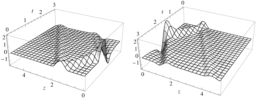
Figure 1: Example 1, two views of $\phi(t,z)$.

5.1.2 Example 2

In this case, interchanging the roles of $f$ and $g$, we set

$$f(z)=0\quad\quad\quad\mbox{and}\quad\quad\quad g(z)=\cases{0&$0\leq z\leq 1$\\ 16(z-1)^{2}(z-2)^{2}\quad\quad&$1\leq z\leq 2$\\ 0&$2\leq z$}\,.$$

In Fig. 2 we display two views of the plot of $\phi(t,z)$ for $t\in[0,3]$ and $z\in[0,5]$ obtained from (38) and (5.1). In this case, we readily get from (40) that $\phi(t,0)$ tends to $0$ as $C/t$. We can see from Fig. 2, that the wave is also completely reflected at the boundary.

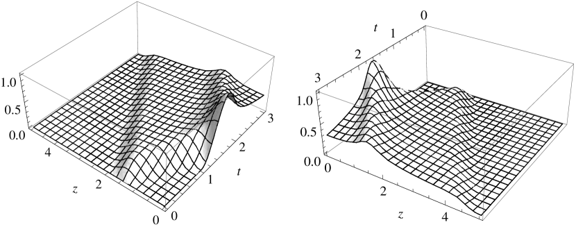
Figure 2: Example 2, two views of $\phi(t,z)$.

These examples clearly show that, in spite of $\phi(t,z)$ does not satisfy any prescribed boundary condition at the origin, some of the qualitative features of the waves are similar to those of the classical cases, such as vibrating strings or pressure waves in pipes, with boundary condition imposed at the end. In fact, in all the cases the original pulse decomposes in two pieces and the one travelling to the boundary completely reflects at it.

However, in the latter cases, the corresponding operator $A$ does not satisfy the well-posedness property and admits infinitely many self-adjoint extensions with domain included in the energy space. For instance, the propagation of pressure waves inside the tube of a wind musical instrument depends drastically on the physical properties of its end. When it is open, the air pressure must equal the atmospheric pressure there, and we have to impose Dirichlet’s boundary conditions. Being the end closed, air cannot move at it, and Neumann’s boundary conditions must be required. Furthermore, by adding a movable membrane at the extreme, we can generate more general boundary conditions to be satisfied. Therefore, in these cases, it is Physics which requires the existence of infinitely many self-adjoint extensions.

Whereas, in our case, in which Physics cannot provide any boundary condition to be imposed, the alternative well-posedness property fortunately tells us that none is actually needed.

6 Schwarzschild with negative mass

The analysis of Schwarzschild spacetime with negative mass shows similar features than Taub’s example, and it is the purpose of this section to briefly describe it.

We start with recalling the geometrical setting. The space is $\Omega=S^{2}\times(0,\infty)$ and the metric of the spacetime is

$$ds^{2}=-\left(1+\frac{2M}{r}\right)dt^{2}+\left(1+\frac{2M}{r}\right)^{-1}dr^{2}+r^{2}d\Sigma^{2},$$

where $d\Sigma^{2}$ denotes the metric on the unit sphere $S^{2}$ and $M$ is a positive parameter. In this case, the wave equation writes

$$\partial_{tt}\phi+A\phi=0$$

with

$$A\varphi=-\left(1+\frac{2M}{r}\right)\frac{1}{r^{2}}\,\left[\partial_{r}\left(r^{2}\left(1+\frac{2M}{r}\right)\partial_{r}\varphi\right)+\Delta_{S^{2}}\varphi\right]$$

defined on $C_{0}^{\infty}(\Omega)$.

The operator $A$ is symmetric on the Hilbert space

$$H=\{\varphi(r,\mathbf{\theta}):\int_{\Omega}|\varphi(r,\mathbf{\theta})|^{2}\frac{r^{2}}{1+\frac{2M}{r}}drd\sigma(\mathbf{\theta}\ ,)<\infty\}$$

and the associated energy space is defined as in (3), through the sesquilinear form

$$b(\varphi,\eta)=\int_{\Omega}\partial_{r}\varphi\ \partial_{r}\eta\ r^{2}\Big{(}1+\frac{2M}{r}\Big{)}drd\sigma(\mathbf{\theta})+\int_{\Omega}\nabla_{\mathbf{\theta}}\varphi\cdot\nabla_{\mathbf{\theta}}\,\eta\ r^{2}drd\sigma(\mathbf{\theta})\ .$$

Theorem 6.1

The operator $A$ is not essentially self-adjoint. However, it has only one self-adjoint extension with domain included in $\mathcal{E}$.

Proof :   The uniqueness of the self-adjoint extension with domain included in $\mathcal{E}$ is proved as in Theorem 2.2. We first show that $C_{0}^{\infty}$ is dense in $\mathcal{E}$, just by mimicking the proof of Lemma 3.1, and then we usethe same argument to conclude. The counterexample to essential self-adjointness is given by any function

$$\varphi(r,\mathbf{\theta})=Q_{l}\left(1+\frac{r}{M}\right)Y_{l}^{m}(\mathbf{\theta})$$

where $\theta\in S^{2}$ is the current point in the unit sphere, $l$ is an integer, $l\geq 1$, $m$ is another integer with $|m|\leq l$, $Y_{l}^{m}$ is the spherical harmonic, and $Q_{l}$ is the second Legendre function. We recall that $Q_{l}\big{(}1+\frac{r}{M}\big{)}=O(|\ln r|)$ and $Q_{l}^{\prime}\big{(}1+\frac{r}{M}\big{)}=O(\frac{1}{r})$ when $r\rightarrow 0$, while $Q_{l}\big{(}1+\frac{r}{M}\big{)}=O(r^{-l-1})$ at infinity. Hence, $\varphi_{l,m}\in H$, but $\varphi_{l,m}\notin\mathcal{E}$ on one hand, on the other hand, $A^{*}\varphi_{l,m}=0$ by construction.

$\Box$

The example $\varphi(r,\mathbf{\theta})=(1+Y_{l}^{m}(\mathbf{\theta}))\eta(r)$ shows that functions in the domain of $A$ do not necessarily have a trace at the origin. This comes from the dependency with respect to angular variables. However, if we consider for each $\varphi$ in the domain of $A$ its mean values over the spheres $S(0,r)$, angular variables disappear and, as a result the limit when $r\to 0$ does exists, and is not a priori vanishing. Indeed, we have the following.

Theorem 6.2

Let $\varphi\in D(A)$ and define

$$\lambda(\varphi,r)=\int_{S^{2}}\varphi(r,\mathbf{\theta})d\sigma(\mathbf{\theta}).$$

Then,

$$\lim_{r\to 0}\lambda(\varphi,r)=:\lambda(\varphi)$$

exists, and

$$|\lambda(\varphi)|\leq C(\|A\varphi\|_{H}+\|\varphi\|_{\mathcal{E}})$$

for some constant $C$.

Proof :   Let $\varphi\in D(A)$, $\psi\in H$ such that $\psi=A\varphi$; multiplying it by a cut-off function away from zero, we assume that Supp $\varphi\subset B(0,1)$. We have

$$-\left(1+\frac{2M}{r}\right)\frac{1}{r^{2}}\,\left[\partial_{r}\left(r^{2}\left(1+\frac{2M}{r}\right)\partial_{r}\lambda(\varphi,r)\right)\right]=\int_{S^{2}}\psi(r,\mathbf{\theta})d\sigma(\mathbf{\theta})$$

$$+\left(1+\frac{2M}{r}\right)\frac{1}{r^{2}}\int_{S^{2}}\Delta_{S^{2}}\varphi(r,\mathbf{\mathbf{\theta}})d\sigma(\mathbf{\theta}))$$

$$=\int_{S^{2}}\psi(r,\mathbf{\theta})d\sigma(\mathbf{\theta}),$$

from which we deduce that

$$\int_{0}^{1}\left|\partial_{r}\left(r^{2}\left(1+\frac{2M}{r}\right)\partial_{r}\lambda(\varphi,r)\right)\right|^{2}\left(1+\frac{2M}{r}\right)\frac{dr}{r^{2}} \leq \int_{\Omega}|\psi(r,\theta)|^{2}r^{2}\frac{drd\sigma(\mathbf{\theta})}{1+\frac{2M}{r}}$$

$$\leq C\|\psi,,-\|_{H}.$$

Using this estimate and Cauchy-Schwarz inequality, we obtain for $s<r<1$

$$\left|r^{2}\left(1+\frac{2M}{r}\right)\partial_{r}\lambda(\varphi,r)-s^{2}\left(1+\frac{2M}{s}\right)\partial_{s}\lambda(\varphi,s)\right|$$

$$\leq C\left(\int_{s}^{r}\frac{t^{2}}{1+\frac{2M}{t}}dt\right)^{\frac{1}{2}}\|\psi\|_{H}.$$ (41)

Then ${\displaystyle\lim_{r\to 0}r^{2}\left(1+\frac{2M}{r}\right)\partial_{r}\lambda(\varphi,r)}$ exists and it must be zero since

$$\int_{0}^{1}|\partial_{r}\lambda(\varphi,r)|^{2}rdr<\infty.$$

Thus, when $s$ goes to $0$, we get from (6) that

$$|\partial_{r}\lambda(\phi,r)|\leq Cr\left(\int_{0}^{r}|\psi(t,\theta)|^{2}dt\right)^{\frac{1}{2}}.$$

Hence

$$\lambda(\varphi,0)=-\int_{0}^{1}\partial_{r}\lambda(\varphi,r)dr$$

exists when $\mbox{Supp}\ \varphi\subset B(0,1)$. The end of the proof follows as in the proof of (16).

$\Box$

Remark. Non essential self-adjointness of $A$ has been claimed in [2] where a different argument based on von Neumann’s criterion is suggested. However we think preferable to give a proof.

Later on, the authors of [3] suggested to replace the underlying Hilbert space $H$ by the energy space $\mathcal{E}$. To avoid confusion, we note $A_{\mathcal{E}}$ their operator, given by (6), defined on $C_{0}^{\infty}$ and taking values in $\mathcal{E}$. They claimed that, doing this, the operator $A_{\mathcal{E}}$ is essentially self-adjoint. This is not founded for three reasons. First, the energy which is associated to such an operator is not the physical energy. Second, the importance of the density in $\mathcal{E}$ of $C_{0}^{\infty}$ has been skipped in [3], while it is a key property which must be verified, otherwise the operator $A$ would not be densely defined (a non densely defined operator cannot be essentially self-adjoint). Finally, and more dramatically, their claimed result is just false.

Indeed, by Theorem 6.2 there exists a non trivial linear form on $D(A)$ which vanishes on $C_{0}^{\infty}$. Hence the closure of the latter in the former, which we denote by $D_{0}$, is strictly included in $D(A)$. One can use this to construct two different self-extensions of $A_{\mathcal{E}}$. Let $\beta$ be the sesquilinear form associated to $A_{\mathcal{E}}$ with domain $D(A)$, and $\beta_{0}$ the analogous form with domain $D_{0}$. Then, we classically define $\mathcal{A}$ and $\mathcal{A}_{0}$ respectively on:

$$D(\mathcal{A})=\{f\in D(A);\,\forall g\in D(A)\,|\beta(f,g)|\leq C\|g\|_{\mathcal{E}}\}$$

and

$$D(\mathcal{A}_{0})=\{f\in D_{0};\,\forall g\in D_{0}\,|\beta(f,g)|\leq C\|g\|_{\mathcal{E}}\},$$

where

$$\beta(f,\psi)=<Af,A\psi>_{H}.$$

Both are self-adjoint extensions of $A_{\mathcal{E}}$, and there are different since their associated forms have distinct domains.

Part II. The alternative well-posedness property

7 Setting of the problem and statement of the main result

In this second part, we initiate the program which aims at understanding what is hidden behind the examples of the first part, and to which extent one can obtain general results.

We keep on considering $\Omega=\mathbb{R}^{n}\times(0,\infty)$, and turn our attention to the divergence operators of the form

$${L=-\frac{1}{m}\,\mbox{div}\,M\,\mbox{grad}}.$$

We assume:

• (H1) $m\in C^{\infty}(\Omega)$ and $M\in C^{\infty}(\Omega,\mathcal{M}_{n+1}(\mathbb{R}))$;  
  

• (H2) $\displaystyle{\mbox{for all}\ (x,z)\in\Omega\ \ m(x,z)>0\,\ \mbox{and}\ M(x,z)=M(x,z)^{t}>0;}$  
  

• (H3) $m$ and $M$ are integrable on every compact subset of $\bar{\Omega}$.

We define the Hilbert space

$$H=\{\varphi\in L^{2}_{loc}(\Omega):\int_{\Omega}|\varphi(x,z)|^{2}m(x,z)d\mu<\infty\},$$

and the energy space

$$\mathcal{E}=\{\varphi\in H\cap H^{1}_{\mbox{loc}}(\Omega):b(\varphi,\varphi)<\infty\},$$

where

$$b(\varphi,\psi)=\int_{\Omega}M(x,z)\,\mbox{grad}\,\varphi(x,z)\cdot\mbox{grad}\,\psi(x,z)\,d\mu$$ (42)

for suitable $\varphi,\psi$. They are equipped with their canonical norms. Thanks to hypothesis (H3), $C_{c}^{\infty}(\Omega)$ is included in $H$ and $\mathcal{E}$, and we moreover assume

• (H4) $C_{c}^{\infty}(\Omega)$ is dense in $H$ and in $\mathcal{E}$.

Then, the operator $L$ is defined on $C_{0}^{\infty}(\Omega)$ and it is symmetric by (H2). So, we ask when $L$ has the property we call alternative well-posedness, which, by definition, means that there is only one self-adjoint extension of $L$ with domain included in $\mathcal{E}$. A first answer to this question is the following result.

Theorem 7.1

Let $L$ be a divergent operator fulfilling hypotheses (H1-H4)

1. Assume $L$ has the alternative well-posedness property. Then, for every measurable and non negligible set $\Gamma$ in $\mathbb{R}^{n}$, we have

   $$\int_{0}^{1}\int_{\Gamma}\frac{1}{m_{n+1,n+1}(x,z)}dx\,dz=\infty.\ \$$ (43)

2. Assume that for all $x\in\mathbb{R}^{n}$(everywhere, not almost everywhere) there exists an open ball $B$ containing $x$ such that

   $$\int_{0}^{1}\frac{1}{\omega_{B}(z)}dz=\infty,\ \$$ (44)

   where $\omega_{B}(z)=\int_{B}m_{n+1,n+1}(y,z)dy$. Then $L$ has the alternative well-posedness property.

This theorem says that only the normal diagonal part of $L$, namely the term $-\partial_{z}m_{n+1,n+1}\partial_{z}$, seems to matter with respect to the alternative well-posedness and that it should vanish rapidly enough on approaching the boundary for this property to hold.  
The necessary condition in (i) is not sufficient: there exists an operator $L$ which does not have the alternative well-posedness, but such that

$$\int_{0}^{1}\int_{\Gamma}\frac{1}{m_{n+1,n+1}(x,z)}dx\,dz=\infty\ \$$ (45)

for every non negligible subset $\Gamma$ of $\mathbb{R}^{n}$.

Also, the sufficient condition in (ii) is not necessary: there exists an operator $L$ which has the alternative well-posedness, but such that

$$\int_{0}^{1}\frac{1}{\omega_{B}(z)}dz<\infty\ \$$ (46)

for all balls $B$ containing the origin. However, this condition is sharp in the sense that there exists an operator $L$ which has not the alternative well-posedness property, satisfying (44) for every $x\in\mathbb{R}^{n}$ but $0$.

Nevertheless, an immediate and useful corollary, which in particular applies when $m_{n+1,n+1}$ only depends on the variable $z$, is the following. Its proof is left to the reader.

Corollary 7.2

Assume, in addition, that for all $x\in\mathbb{R}^{n}$ there exists $\rho>0$ such that

$$\sup_{z\leq 1}\left(\int_{B(x,\rho)}m_{n+1,n+1}(y,z)dy\right)\left(\int_{B(x,\rho)}\frac{1}{m_{n+1,n+1}(y,z)}dy\right)<\infty.$$ (47)

Then $L$ has the alternative well-posedness property if and only if, for all balls $B$ in $\mathbb{R}^{n}$, we have

$$\int_{0}^{1}\int_{B}\frac{1}{m_{n+1,n+1}(y,z)}dy\,dz=\infty.$$ (48)

A remark is here in order. The reader has noticed that our hypothesis (H1) on the regularity of the coefficients is obviously not sharp. They are designed to avoid additional difficulties which are not essential for our understanding of the alternative well-posedness property.

8 Proof of Theorem 7.1

We begin with an abstract characterization of the alternative well-posedness property. Let us denote by $\mathcal{E}_{0}$ the closure of $C_{0}^{\infty}(\Omega)$ in $\mathcal{E}$. Then, we have

Lemma 8.1

The operator $L$ has the alternative well-posedness property if and only if $\mathcal{E}_{0}=\mathcal{E}$.

To prove this assertion, we begin with assuming that $L$ has the alternative well-posedness property. Let $\mathcal{L}$ and $\mathcal{L}_{0}$ be the self-adjoint operators associated with the form $b$ given by (42) and defined on domains $\mathcal{E}$ and $\mathcal{E}_{0}$ respectively. They are both extensions of $L$ with domains included in $\mathcal{E}$, and so, are equal. But then we must have $D(\mathcal{L}^{\frac{1}{2}})=D(\mathcal{L}_{0}^{\frac{1}{2}})$, which is $\mathcal{E}=\mathcal{E}_{0}$.

Reciprocally, if $\mathcal{E}=\mathcal{E}_{0}$, the only self-adjoint extension of $L$ with domain in $\mathcal{E}$ is its Friedrichs extension, because the form $b$ defined on $\mathcal{E}$ is the closure of the form $b$ defined on $C_{0}^{\infty}(\Omega)$. The lemma is proved.

$\Box$

Remark 8.2

This Lemma, as simple as it is, enlightens the key point in the alternative well-posedness property. Indeed, in a classical case where boundary conditions are needed, the space $\mathcal{E}$ is the largest possible Banach space onto which $(b(\varphi,\varphi)+\|\varphi\|^{2}_{H})^{\frac{1}{2}}$ defines a norm, while $\mathcal{E}_{0}$ is the smallest one containing $C^{\infty}_{0}(\Omega)$. One thus may understand the alternative well-posedness as saying that the smallest possible space is also the largest, and this is why no boundary condition is needed to obtain a self-adjoint extension with domain in $\mathcal{E}$.

We turn to the proof of the first assertion of Theorem 7.1. We assume the existence of a non negligible subset $\Gamma$ of $\mathbb{R}^{n}$ such that

$$\int_{0}^{1}\int_{\Gamma}\frac{1}{m_{n+1,n+1}(x,z)}\,dx\,dz<\infty.\ \$$ (49)

We will prove that $\mathcal{E}_{0}\neq\mathcal{E}$ by constructing a linear form on $\mathcal{E}$ vanishing on $\mathcal{E}_{0}$, but not identically vanishing.

Let $\eta\in C_{c}^{\infty}(0,\frac{1}{2})$ which equals 1 in a neighbourhood of $0$. If $\varphi\in\mathcal{E}$ we set

$$\lambda(\varphi)=\int_{0}^{1}\int_{\Gamma}\partial_{z}(\varphi(x,z)\eta(z))dx\,dz.$$

That $\lambda$ defines a continuous linear form on $\mathcal{E}$ follows directly from Cauchy-Schwarz inequality and (49); it is vanishing on $\mathcal{E}_{0}$ but not on $\mathcal{E}$, since $\lambda(\varphi)=-\int_{\Gamma}\varphi(x,0)dx$ whenever $\varphi\in C_{c}^{\infty}(\Omega)$.

Regarding the second assertion, we assume $\mathcal{E}\neq\mathcal{E}_{0}$ and prove that (44) does not hold. There exists $\lambda\in\mathcal{E}^{\prime}$ (the dual space of $\mathcal{E}$), not identically vanishing, but null on $\mathcal{E}_{0}$. Therefore, there is at least one (and in fact many, as we will see) test function $\varphi\in C_{c}^{\infty}(\Omega)$ such that $\lambda(\varphi)\neq 0$.

The first step consists in showing that whenever $\lambda(\varphi)\neq 0$ (suppose $\lambda(\varphi)=1$), then $\int_{0}^{1}\frac{1}{\omega_{B}}<\infty$ as soon as $B\supset\mbox{Supp}\ \phi(\cdot,0)$. For $x\in\mathbb{R}^{n}$, we write $\zeta_{0}(x)=\varphi(x,0)$ and we define

$$E=\{\eta\in H^{1}_{loc}(0,\infty):\ \zeta_{0}\otimes\eta\in\mathcal{E}\},$$

equipped with the norm $\displaystyle{\|\eta\|_{E}=\|\zeta_{0}\otimes\eta\|_{\mathcal{E}}}.$ It is a Banach space, on which $C_{c}^{\infty}(0,\infty)$ is dense.

Let $\eta\in C_{c}^{\infty}(0,\infty)$ and $\psi=\eta(0)\varphi-\zeta_{0}\otimes\eta$. Since $\psi$ vanishes on $\partial\Omega$, it belongs to $\mathcal{E}_{0}$ (extend it by $0$ outside $\Omega$ and remark that $\psi_{\varepsilon}(x,z)=\psi(x,z-\varepsilon)$ converge towards $\psi$ in $\mathcal{E}$). We thus have

$$\lambda(\zeta_{0}\otimes\eta)=\lambda(\eta(0)\varphi)=\eta(0)$$

and

$$|\eta(0)|\leq\|\lambda\|_{\mathcal{E}^{\prime}}\|\eta\|_{E}.$$ (50)

We compute

$$\|\eta\|_{E}^{2}=\int_{0}^{\infty}\omega(z)\eta^{\prime}(z)^{2}\,dz+\int_{0}^{\infty}\beta(z)\eta^{\prime}(z)\eta(z)\,dz+\int_{0}^{\infty}(\alpha(z)+c(z))\eta(z)^{2}\,dz$$

where, decomposing the matrix $M$ as

$$M=\left(\begin{array}[]{ccccc}&&&&m_{1,n+1}\\ &&&&.\\ &&M^{\prime}&&.\\ &&&&.\\ m_{1,n+1}&.&.&.&m_{n+1,n+1}\end{array}\right),$$

we have set

$$\omega(z) = \int_{\mathbb{R}^{n}}m_{n+1,n+1}(x,z)\zeta_{0}(x)^{2}\,dx,$$

$$\beta(z) = 2\sum_{j=1}^{n}\int_{\mathbb{R}^{n}}m_{j,n+1}(x,z)\partial_{j}\zeta_{0}(x)\zeta_{0}(x)\,dx,$$

$$\alpha(z) = \int_{\mathbb{R}^{n}}M^{\prime}(x,z)\nabla\zeta_{0}(x)\cdot\nabla\zeta_{0}(x)\,dx,$$

$$c(z) = \int_{\mathbb{R}^{n}}\zeta_{0}(x)^{2}\,m(x,z)\,dx.$$

By the positive definiteness of $M$, we have for all $z>0$

$$\beta(z)\leq 2\sqrt{\alpha(z)\omega(z)}.$$

Inserting this in (50), we find that

$$|\eta(0)|^{2}\leq C\left(\int_{0}^{\infty}w(z)\eta^{\prime}(z)^{2}\,dz+\int_{0}^{\infty}(\alpha(z)+c(z))\eta(z)^{2}\,dz\right)$$

for some uniform constant $C$. It is not difficult to see that this last inequality implies

$$\int_{0}^{1}\frac{1}{w(z)}\,dz\leq C,$$

and then

$$\int_{0}^{1}\frac{1}{\omega_{B}(z)}\,dz<\infty,$$ (51)

for all balls $B$ which contain the support of $\zeta_{0}$.

The second step is an argument of descent which will give one point $x$ in $\mathbb{R}^{n}$ such that (51) holds when $B$ contains $x$. We will use for each $j\geq 0$ a partition of unity $(\chi_{j,k})_{k\in\mathbb{Z}^{n}}$with $\mbox{Supp}\ \chi_{j,k}\subset B(k2^{-j},\sqrt{n}2^{-j})=:B_{j,k}$.

We start with $j=0$, and decompose $\varphi=\sum_{k}\varphi\chi_{0,k}$. There must exist at least one $k_{0}\in\mathbb{Z}^{n}$ such that $\lambda(\varphi\chi_{0,k_{0}})\neq 0$. By the first step, the inequality (51) is verified for $B=B_{0,k_{0}}$.

We now decompose $\varphi_{0}=\varphi\chi_{0,k_{0}}$ at the next finer scale: $\varphi_{0}=\sum_{k}\varphi_{0}\chi_{1,k}$, and select $k_{1}$ such that $\lambda(\varphi_{0}\chi_{1,k_{1}})\neq 0$. Then, (51) holds for $B=B_{1,k_{1}}$ (note that this ball is included in $B_{0,k_{0}}$).

We continue, and thus inductively construct a nested sequence of dyadic balls fulfilling (51): the point $x$ we are looking for is at the intersection of these balls. Theorem 7.1 is completely proved.

9 A few conclusive words

Going back to spacetimes with naked singularities, the alternative well posedness property being satisfied means that such spacetimes, though exhibiting a boundary, are physically consistent because their Laplace-Beltrami operator is well defined without requiring any condition at the boundary. We are not claiming that naked singularities do exist in the universe, which we do not know. But, at least, the necessity to define a condition at the boundary, fortunately, does not exist.

However we have proved the alternative well-posedness property only for the examples of this paper. If we believe in General Relativity, then it is conceivable that any meaningful solution having naked singularities should fulfill the alternative well-posedness property.

Appendix A Proof of Proposition 5.1

Since the characteristics of the equation (37) are $z\pm t=$ constant, the change of variables $\xi=z+t$ and $\eta=z-t$ brings this equation to $L(\phi)=0$, where

$$L(\phi)=\partial_{\xi\eta}\phi+\frac{1}{2(\xi+\eta)}(\partial_{\xi}\phi+\partial_{\eta}\phi).$$

The adjoint $L^{*}$ of the operator $L$ is given by

$$L^{*}(\psi)=\partial_{\xi\eta}\psi-\partial_{\xi}\left(\frac{\psi}{2(\xi+\eta)}\right)-\partial_{\eta}\left(\frac{\psi}{2(\xi+\eta)}\right)$$ (52)

and we have

$$\psi L(\phi)-\phi L^{*}(\psi)=-\partial_{\xi}\left(\phi\;\partial_{\eta}\psi-\frac{\phi\,\psi}{2(\xi+\eta)}\right)+\partial_{\eta}\left(\partial_{\xi}\phi\;\psi+\frac{\phi\,\psi}{2(\xi+\eta)}\right).$$

Taking $\phi$ such that $L(\phi)=0$ and integrating over a piecewise smooth compact domain $\Gamma$ with boundary $\partial\Gamma$, one obtains by Green’s formula

$$-\int\int_{\Gamma}\phi L^{*}(\psi)\,d\xi\,d\eta=\oint_{\partial\Gamma}\left(\partial_{\xi}\phi\;\psi\,d\xi+\phi\,\partial_{\eta}\psi\,d\eta+\frac{\phi\,\psi}{2(\xi+\eta)}(d\xi-d\eta)\right)\,,$$ (53)

where the line integral around $\partial\Gamma$ is taken in the clockwise sense.

To obtain a representation for $\phi(P)=\phi(\xi_{0},\eta_{0})$, following Riemann (see, for example, [16]), we choose for $\psi$ a function $R(\xi,\eta;\xi_{0},\eta_{0})$ subject to the following conditions:

a) As a function of $\xi$ and $\eta$, $R$ satisfies the adjoint equation

$$L_{(\xi,\eta)}^{*}(R)=0\,.$$

b) On the characteristics $\eta=\eta_{0}$ and $\xi=\xi_{0}$ it satisfies

$$\partial_{\xi}R-\frac{R}{2(\xi+\eta)}=0\hskip 56.9055pt{\rm on}\hskip 14.22636pt\eta=\eta_{0}\,,$$

and

$$\partial_{\eta}R-\frac{R}{2(\xi+\eta)}=0\hskip 56.9055pt{\rm on}\hskip 14.22636pt\xi=\xi_{0}\,.$$

c) $R(\xi_{0},\eta_{0};\xi_{0},\eta_{0})=1$.

Conditions b) are ordinary differential equations along the characteristics; integrating them and using c) we get that

$$R(\xi,\eta;\xi_{0},\eta_{0})=\sqrt{\frac{\xi+\eta}{\xi_{0}+\eta_{0}}}\,.$$

on both characteristics.

Now by trying with the ansatz

$$R(\xi,\eta;\xi_{0},\eta_{0})=\sqrt{\frac{\xi+\eta}{\xi_{0}+\eta_{0}}}\,F(w)\,,$$

where

$$w=-\frac{(\xi-\xi_{0})(\eta-\eta_{0})}{(\xi_{0}+\eta_{0})(\xi+\eta)}\,,$$ (54)

and using (52) we get that in order to satisfy condition a) the function $F(w)$ must satisfy the differential equation

$$w(1-w)F^{\prime\prime}(w)+(1-2w)F^{\prime}(w)-\frac{1}{4}F(w)=0\,.$$ (55)

The only solution of this equation with $F(0)=1$ is the Gauss hypergeometric function $\;{}_{2}F_{1}\,(\frac{1}{2},\frac{1}{2};{1};w)$ [17]. Therefore we have that the Riemann function is

$$R(\xi,\eta;\xi_{0},\eta_{0})=\sqrt{\frac{\xi+\eta}{\xi_{0}+\eta_{0}}}\,\;_{2}F_{1}\!\left(\frac{1}{2},\frac{1}{2};{1};-\frac{(\xi-\xi_{0})(\eta-\eta_{0})}{(\xi_{0}+\eta_{0})(\xi+\eta)}\right)\,,$$ (56)

which is a $C^{\infty}$ function of $\xi$ and $\eta$, for $\xi+\eta>0$, $\xi_{0}+\eta_{0}>0$ and $|w|<1$.

It can be shown that as a function of $\xi_{0}$ and $\eta_{0}$, $R$ also satisfies the equation

$$L_{(\xi_{0},\eta_{0})}(R)=0\,.$$

For the sake of clearness, we introduce new time-like coordinates $t=(\xi_{0}-\eta_{0})/2$ and $\tau=(\xi-\eta)/2$ and spacelike ones $z=(\xi_{0}+\eta_{0})/2$ and $\zeta=(\xi+\eta)/2$. In terms of these coordinates, we have

$$w=\frac{(t-\tau)^{2}-(z-\zeta)^{2}}{4z\zeta}\,,$$

and

$$R(\tau,\zeta;t,z)=\sqrt{\frac{\zeta}{z}}\,\;_{2}F_{1}\!\left(\frac{1}{2},\frac{1}{2};{1};\frac{(t-\tau)^{2}-(z-\zeta)^{2}}{4z\zeta}\right)\,.$$ (57)

Figure 3: Domain of integration $\Gamma$: (a) for $z>t$ and (b) for $z<t$.

It can readily be seen from (54) that, in the region $0\leq\xi\leq\xi_{0}$, $\eta\geq\eta_{0}$, $\xi+\eta>0$ and $\xi_{0}+\eta_{0}>0$ (see Fig. 3), it holds that $w\geq 0$. If in addition $\eta_{0}>0$ ($z>t$), we can easily check that $0\leq w<1$ and then Riemann’s function (56) is well-defined in that region. However, if $\eta_{0}<0$ ($z<t$), we see that $w=1$ on the characteristic $\xi=-\eta_{0}$, and furthermore $w>1$ for $0\leq\xi<-\eta_{0}$. Thus, in the latter case, $R(\xi,\eta;\xi_{0},\eta_{0})$ is defined through (56) only for $-\eta_{0}<\xi\leq\xi_{0}$.

Therefore we must treat the cases $z>t$ and $z<t$ separately.

A.1 $z>t$

In this case, since $R(\xi,\eta;\xi_{0},\eta_{0})$ is an infinitely differentiable solution of $L_{(\xi,\eta)}^{*}(\psi)=0$ in $0\leq\xi\leq\xi_{0}$ and $\eta\geq\eta_{0}$, by applying expression (53) to the triangle $ABP$ (see Fig.3(a)) we get

$$\int_{AB}\left(\partial_{\xi}\phi\;R\,d\xi+\phi\,\partial_{\eta}R\,d\eta+\frac{\phi\,R}{2(\xi+\eta)}(d\xi-d\eta)\right)$$

$$+\int_{BP}\phi\,\left(\partial_{\eta}R-\frac{R}{2(\xi+\eta)}\right)d\eta+\int_{PA}\left(\partial_{\xi}\phi\;R+\frac{\phi\,R}{2(\xi+\eta)}\right)d\xi = 0\,,$$

since $d\xi=d\eta$ along $AB$ and

$$\int_{PA}\partial_{\xi}\phi\,R\,d\xi=\phi(A)R(A)-\phi(P)R(P)-\int_{PA}\phi\,\partial_{\xi}R\,d\xi\,,$$

we have

$$\int_{AB}\left(\partial_{\xi}\phi\;R\,d\xi+\phi\,\partial_{\eta}R\,d\eta\right)+\int_{BP}\phi\,\left(\partial_{\eta}R-\frac{R}{2(\xi+\eta)}\right)d\eta$$

$$+\phi(A)R(A)-\phi(P)R(P)-\int_{PA}\phi\;\left(\partial_{\xi}R-\frac{R}{2(\xi+\eta)}\right)d\xi = 0\,.$$

Taking into account that $R$ satisfies conditions b) and c), we get Riemann’s representation formula

$$\phi(P)=\phi(A)R(A)+\int_{AB}\left(\partial_{\xi}\phi\;R\,d\xi+\phi\,\partial_{\eta}R\,d\eta\right)\,.$$

In order to obtain a more symmetric expression, we add the identity

$$0=\frac{1}{2}\bigl{(}\phi(B)R(B)-\phi(A)R(A)\bigr{)}-\frac{1}{2}\int_{AB}\bigl{(}\partial_{\xi}(\phi R)\,d\xi+\partial_{\eta}(\phi R)\,d\eta\bigr{)}\,$$

getting

$$\phi(P) = \frac{1}{2}\bigl{(}\phi(B)R(B)+\phi(A)R(A)\bigr{)}$$

$$+ \frac{1}{2}\int_{AB}\bigl{(}\partial_{\xi}\phi\;R-\phi\;\partial_{\xi}R\,\bigr{)}d\xi-\frac{1}{2}\int_{AB}\bigl{(}\partial_{\eta}\phi\,R-\phi\,\partial_{\eta}R\bigr{)}\,d\eta\,.$$

Finally, by using (57) we get (38).

A.2 $z<t$

In this case, $R(\xi,\eta;\xi_{0},\eta_{0})$ is an infinitely differentiable solution of $L_{(\xi,\eta)}^{*}(\psi)=0$ in $-\eta_{0}<\xi\leq\xi_{0}$ and $\eta\geq\eta_{0}$. For $\epsilon>0$ and sufficiently small, let us consider the trapezium $A_{+}BPC_{+}A_{+}$ with vertices $A_{+}=(-\eta_{0}+\epsilon,-\eta_{0}+\epsilon)$, $B=(\xi_{0},\xi_{0})$, $P=(\xi_{0},\eta_{0})$ and $C_{+}=(-\eta_{0}+\epsilon,\eta_{0})$ (see Fig.3(b)), by using expression (53) we have

$$0=\oint_{A_{+}BPC_{+}A_{+}}\left(\partial_{\xi}\phi\;R\,d\xi+\phi\,\partial_{\eta}R\,d\eta+\frac{\phi\,R}{2(\xi+\eta)}(d\xi-d\eta)\right)\,,$$

and proceeding as in the $z>t$ case we get

$$\phi(P) = \phi(C_{+})R(C_{+})+\int_{A_{+}B}\left(\partial_{\xi}\phi\;R\,d\xi+\phi\,\partial_{\eta}R\,d\eta\right)$$

$$+ \int_{C_{+}A_{+}}\phi\,\left(\partial_{\eta}R-\frac{R}{2(\xi+\eta)}\right)d\eta\,.$$

Now, taking into account that

$$_{2}F_{1}\,\left(\frac{1}{2},\frac{1}{2};{1};1-\theta\right)=-\frac{1}{\pi}\log\left(\frac{\theta}{16}\right)-\frac{1}{4\pi}\left(\log\left(\frac{\theta}{16}\right)+2\right)\theta+O\left(\theta^{2}\,\log\theta\right),$$ (58)

a straightforward computation from (56) shows that, on the characteristic $C_{+}A_{+}$, i.e., $\xi=-\eta_{0}+\epsilon$,

$$\left(\partial_{\eta}R-\frac{R}{2(\xi+\eta)}\right)\Bigg{|}_{\xi=-\eta_{0}+\epsilon}=\frac{1}{\pi(\xi_{0}+\eta)}\sqrt{\frac{\xi_{0}+\eta_{0}}{\eta-\eta_{0}}}+O(\epsilon\,\ln\epsilon)\,.$$

Therefore we have

$$\phi(P) = \phi(C_{+})\sqrt{\frac{\epsilon}{\xi_{0}+\eta_{0}}}\,+\int_{A_{+}B}\left(\partial_{\xi}\phi\;R\,d\xi+\phi\,\partial_{\eta}R\,d\eta\right)$$

$$+ \frac{1}{\pi}\int_{C_{+}A_{+}}\frac{\phi}{(\xi_{0}+\eta)}\sqrt{\frac{\xi_{0}+\eta_{0}}{\eta-\eta_{0}}}\;d\eta+O(\epsilon\,\ln\epsilon)\,,$$

and when $\epsilon$ goes to $0$, we get

$$\phi(P)=\int_{AB}\left(\partial_{\xi}\phi\;R\,d\xi+\phi\,\partial_{\eta}R\,d\eta\right)+\frac{1}{\pi}\int_{\eta_{0}}^{-\eta_{0}}\frac{\phi(-\eta_{0},\eta)}{(\xi_{0}+\eta)}\sqrt{\frac{\xi_{0}+\eta_{0}}{\eta-\eta_{0}}}\;d\eta\,.$$ (59)

In order to get rid of the integral along the characteristic $CA$ in the last expression we shall “extend” the Riemann’s function $R$ to the region $w>1$.

Let us consider the function

$$R_{1}(\xi,\eta;\xi_{0},\eta_{0})=\sqrt{\frac{\xi+\eta}{\xi_{0}+\eta_{0}}}\,\frac{1}{\sqrt{w}}\;_{2}F_{1}\!\left(\frac{1}{2},\frac{1}{2};{1};\frac{1}{w}\right)$$

$$=\frac{\xi+\eta}{\sqrt{(\xi_{0}-\xi)(\eta-\eta_{0})}}\,\;_{2}F_{1}\!\left(\frac{1}{2},\frac{1}{2};{1};-\frac{(\xi_{0}+\eta_{0})(\xi+\eta)}{(\xi-\xi_{0})(\eta-\eta_{0})}\right)\,.$$ (60)

Clearly $R_{1}$ vanishes at the boundary ($\xi+\eta=0$) and by comparing with (56), we see that $R$ and $R_{1}$ “formally coincide” at $w=1$, although, of course, none of them exist there (see equation (58)).

On the other hand, since $\displaystyle{\frac{1}{\sqrt{w}}\;_{2}F_{1}\!\left(\frac{1}{2},\frac{1}{2};{1};\frac{1}{w}\right)}$ is the regular solution at $\infty$ of the hypergeometric differential equation (55), $R_{1}$ also satisfies

$$L_{(\xi,\eta)}^{*}(R_{1})=0\hskip 28.45274pt{\rm and}\hskip 28.45274ptL_{(\xi_{0},\eta_{0})}(R_{1})=0\,,$$

as it can be readily checked. Moreover straightforward computations show that in a neighborhood of the boundary

$$\left(\partial_{\eta}R_{1}-\frac{R_{1}}{(\xi+\eta)}\right)\Bigg{|}_{\xi+\eta=\epsilon}=-\frac{\bigl{(}\xi_{0}-\xi+\eta-\eta_{0}\bigr{)}}{4\bigl{(}(\xi_{0}-\xi)(\eta-\eta_{0})\bigr{)}^{3/2}}\;\epsilon+O\left(\epsilon^{2}\right)\,$$ (61)

and that in a neighborhood of the characteristic $CA$

$$\left(\partial_{\eta}R_{1}-\frac{R_{1}}{2(\xi+\eta)}\right)\Bigg{|}_{\xi=-\eta_{0}-\epsilon^{\prime}}=\frac{1}{\pi(\xi_{0}+\eta)}\sqrt{\frac{\xi_{0}+\eta_{0}}{\eta-\eta_{0}}}+O(\epsilon^{\prime}\,\ln\epsilon^{\prime})\,.$$ (62)

For $\epsilon$ and $\epsilon^{\prime}$ positive and small enough, let us consider the triangle $O_{+}A_{-}C_{-}$ with vertices $O_{+}=(\epsilon,\epsilon)$, $A_{-}=(-\eta_{0}-\epsilon^{\prime},-\eta_{0}-\epsilon^{\prime})$ and $C_{-}=(-\eta_{0}-\epsilon^{\prime},\eta_{0}+2\epsilon+\epsilon^{\prime})$ (see Fig.3(b)). Since $R_{1}(\xi,\eta;\xi_{0},\eta_{0})$ is an infinitely differentiable solution of $L_{(\xi,\eta)}^{*}(\psi)=0$ in $\xi+\eta>0$ and $0\leq\xi<-\eta_{0}$, by using expression (53) we have

$$\int_{O_{+}A_{-}}\left(\partial_{\xi}\phi\;R_{1}\,d\xi+\phi\,\partial_{\eta}R_{1}\,d\eta\right)+\int_{A_{-}C_{-}}\phi\,\left(\partial_{\eta}R_{1}-\frac{.R_{1}}{2(\xi+\eta)}\right)d\eta$$

$$+\int_{C_{-}O_{+}}\partial_{\xi}\phi\;R_{1}\,d\xi+\int_{C_{-}O_{+}}\phi\,\left(\partial_{\eta}R_{1}-\frac{R_{1}}{(\xi+\eta)}\right)d\eta=0\,.$$

Taking into account (A.2), (61) and (62) we can write

$$\int_{O_{+}A_{-}}\left(\partial_{\xi}\phi\;R_{1}\,d\xi+\phi\,\partial_{\eta}R_{1}\,d\eta\right)+\frac{1}{\pi}\int_{A_{-}C_{-}}\frac{\phi}{(\xi_{0}+\eta)}\sqrt{\frac{\xi_{0}+\eta_{0}}{\eta-\eta_{0}}}\;d\eta+O(\epsilon,\epsilon^{\prime}\,\ln\epsilon^{\prime})=0\,,$$

and when $\epsilon$ and $\epsilon^{\prime}$ go to $0$, we get

$$\int_{OA}\left(\partial_{\xi}\phi\;R_{1}\,d\xi+\phi\,\partial_{\eta}R_{1}\,d\eta\right)-\frac{1}{\pi}\int_{\eta_{0}}^{-\eta_{0}}\frac{\phi(-\eta_{0},\eta)}{(\xi_{0}+\eta)}\sqrt{\frac{\xi_{0}+\eta_{0}}{\eta-\eta_{0}}}\;d\eta=0\,.$$

Therefore, by adding this expression to (59), we get Riemann’s representation formula for the case $\eta_{0}<0$

$$\phi(P)=\int_{OA}\left(\partial_{\xi}\phi\;R_{1}\,d\xi+\phi\,\partial_{\eta}R_{1}\,d\eta\right)+\int_{AB}\left(\partial_{\xi}\phi\;R\,d\xi+\phi\,\partial_{\eta}R\,d\eta\right)\,.$$

Finally, by using (A.2) we obtain(5.1).

Notice that, since no contribution from the boundary ($\xi+\eta=0$) remains in the last expression, the solution is completely determined by the initial data. Therefore no boundary condition should and can be provided. However, at the boundary, (5.1) becames

$$\phi(t,0) = \int_{0}^{t}\Bigl{(}f^{\prime}(\zeta)+g(\zeta)\Bigr{)}\frac{\zeta}{\sqrt{t^{2}-\zeta^{2}}}\,d\zeta+\,t\int_{0}^{t}\,\frac{f(\zeta)}{(t+\zeta)\;\sqrt{t^{2}-\zeta^{2}}}\,d\zeta\,,$$ (63)

and integrating by parts we get the trace given in (40).

Notice that, for $z=t$, we can easily see that expressions (38) and (5.1) coincide.

$\Box$

References

- [1] Wald R M 1980 J. Math. Phys. 21 2802
- [2] Horowitz G T and Marolf D 1995 Phys. Rev. D 52 5670
- [3] Ishibashi A and Hosoya A 1999 Phys. Rev. D 60 104028
- [4] Ishibashi A and Wald R M 2003 Class. Quantum Grav. 20 3815
- [5] Seggev I 2004 Class. Quantum Grav. 21 2851
- [6] Stalker J G and Shadi Tahvildar-Zadeh A 2004 Class. Quantum Grav. 21 2831
- [7] Taub A H Ann. Math. 1951 53 472
- [8] Liang C 1990 J. Math. Phys. 31 1464
- [9] Gamboa Saraví R E 2008 Int. J. Mod. Phys. A 23 1995
- [10] Gamboa Saraví R E 2009 Gen. Relativ. Gravit. 41 1459
- [11] Gamboa Saraví R E 2009 Int. J. Mod. Phys. A 24 5381
- [12] Gamboa Saraví R E 2008 Class. Quantum Grav. 25 045005
- [13] Gamboa Saraví R E 2004 J. Phys. A: Math. Gen. 37 9573
- [14] Lions J L et Magenes E 1968 Problèmes aux limites non homogènes et applications Volume I, Travaux et Recherches Mathématiques, No. 17 (Dunod, Paris)
- [15] Kato T 1966 Perturbation theory for linear operators (Berlin: Springer-Verlag)
- [16] Courant R and Hilbert D 1962 Methods of Mathematical Physics: Volume II (New York: Interscience)
- [17] Abramowitz M and Stegun I A (eds) 1972 Handbook of Mathematical Functions with Formulas, Graphs, and Mathematical Tables (New York: Dover)