Neighborhoods of univalent functions

Abstract.

The main result shows a small perturbation of a univalent function is again a univalent function, hence a univalent function has a neighborhood consisting entirely of univalent functions.

For the particular choice of a linear function in the hypothesis of the main theorem, we obtain a corollary which is equivalent to the classical Noshiro-Warschawski-Wolff univalence criterion.

We also present an application of the main result in terms of Taylor series, and we show that the hypothesis of our main result is sharp.

1. Introduction

We denote by $U_{r}=\left\{z\in\mathbb{C}:\left|z\right|<r\right\}$ the open disk of radius $r>0$ centered at the origin and we let $U=U_{1}$. The class of functions $f:D\rightarrow\mathbb{C}$ analytic in the domain $D$ will be denoted by $\mathcal{A}\left(D\right)$.

It is known that if $f:D\rightarrow\mathbb{C}$ is a univalent map in a domain $D$, then $f^{\prime}\neq 0$ in $D$. The non-vanishing of the derivative of an analytic function (local univalence) is not in general sufficient to insure the univalence of the function, as it can be seen by considering for example the exponential function $f\left(z\right)=e^{z}$ defined in the upper half-plane.

The classical Noshiro-Warschawski-Wolff univalence criterion gives a partial converse of the above result, as follows:

Theorem 1.1.

If $f:D\rightarrow\mathbb{C}$ is analytic in the convex domain $D$ and

$$\mathop{\rm Re}\nolimits f^{\prime}\left(z\right)>0,\qquad z\in D,$$

then $f$ is univalent in $D$.

In the present paper we introduce the constant $K\left(f,D\right)$ associated with a function $f:D\rightarrow\mathbb{C}$ analytic in a domain $D$, which is a measure of the ”degree of univalence” of $f$ (see Proposition 2.1 and the remark following it).

Using the constant $K\left(f,D\right)$ thus introduced, in Theorem 2.4 we obtain a sufficient condition for univalence, which shows that a small perturbation of a univalent function is again univalent. As a theoretical consequence of this result, it follows that a univalent function has a neighborhood consisting entirely of univalent functions (see Remark 2.8).

The Theorem 2.4 is sharp, in the sense that we cannot replace the upper bound appearing in the hypothesis of this theorem by a larger one, as shown in Example 2.9.

For the particular choice of a linear function in Theorem 2.4, we obtain a simple sufficient condition for univalence (Corollary 2.6), which is shown to be equivalent to the Noshiro-Warschawski-Wolff univalence criterion. The main result in Theorem 2.4 can be viewed therefore as a generalization of this classical result, in which the linear function is replaced by a general univalent function.

The paper concludes with another application of the main result in the case of analytic functions defined in the unit disk. Thus, in Theorem 2.11 and the corollary following it, we obtain sufficient conditions for the univalence of an analytic function defined in the unit disk in terms of the coefficients of its Taylor series representation, which might be of independent interest.

2. Main results

Given a function $f:D\rightarrow\mathbb{C}$ analytic in the domain $D$ we introduce the constant $K\left(f,D\right)$ defined as follows:

(2.1) $$K\left(f,D\right)=\inf_{\begin{subarray}{c}a,b\in D\\ a\neq b\end{subarray}}\left|\frac{f\left(a\right)-f\left(b\right)}{a-b}\right|$$

Note that from the definition follows immediately that if the function $f$ is not univalent in $D$ then $K\left(f,D\right)=0$ The constant $K\left(f,D\right)$ characterizes the univalence of the function $f$ in $D$ in the following sense:

Proposition 2.1.

Let $f:D\rightarrow\mathbb{C}$ be an analytic function in the domain $D$. If $K\left(f,D\right)>0$ then $f$ is univalent in $D$.

Conversely, if $f$ is univalent in $D$ and $\Omega\subset\overline{\Omega}\subset D$ is a domain strictly contained in $D$, then $K\left(f,\Omega\right)>0$.

Proof.

The first statement follows from the inequality

$$\left|f\left(a\right)-f\left(b\right)\right|\geq\left|a-b\right|K\left(f,D\right)>0,$$

for any distinct points $a,b\in D$.

To prove the converse, note that

$$K\left(f,\Omega\right)\geq\inf_{a,b\in\overline{\Omega}}\left|F\left(a,b\right)\right|,$$

where $F:\overline{\Omega}\times\overline{\Omega}\rightarrow\mathbb{C}$ is the function defined by

$$F\left(a,b\right)=\left\{\begin{array}[]{l}\frac{f\left(a\right)-f\left(b\right)}{a-b},\qquad a\neq b\\ f^{\prime}\left(a\right),\qquad\quad a=b\end{array}\right..$$

Note that since $f:D\rightarrow\mathbb{C}$ is analytic, $F$ is continuous on the closed set $\overline{\Omega}\times\overline{\Omega}$, and therefore $F$ attains its minimum modulus on this set:

$$K\left(f,\Omega\right)\geq\inf_{a,b\in\overline{\Omega}}\left|F\left(a,b\right)\right|=\left|F\left(\alpha,\beta\right)\right|,$$

for some $\alpha,\beta\in\overline{\Omega}$.

If $\alpha\neq\beta$, then $\left|F\left(\alpha,\beta\right)\right|=\left|\frac{f\left(\alpha\right)-f\left(\beta\right)}{\alpha-\beta}\right|>0$ since $\alpha,\beta\in\overline{\Omega}\subset D$ and $f$ is univalent in $D$, and if $\alpha=\beta$ then $\left|F\left(\alpha,\alpha\right)\right|=\left|f^{\prime}\left(\alpha\right)\right|>0$, again by the univalence of $f$ in $D$. It follows that in all cases we have

$$K\left(f,\Omega\right)\geq\left|F\left(\alpha,\beta\right)\right|>0,$$

concluding the proof. ∎

Remark 2.2.

Note that the converse in the above proposition may not hold for $\Omega=D$ without the additional hypothesis, as shown in the example below.

In order to have the equivalence

$$f\text{ univalent in }D\Longleftrightarrow\text{ }K\left(f,D\right)>0,$$

one needs additional hypotheses, which guarantee the existence of a continuous extension of $f,f^{\prime}$ to $\overline{D}$, such that $f$ is injective on $\overline{D}$ and $f^{\prime}\neq 0$ in $\overline{D}$.

For example, in the case $D=U$, if the boundary of the image domain $f\left(U\right)$ is a Jordan curve of class $C^{1,\alpha}$ $\left(0<\alpha<1\right)$, by Carathéodory theorem the function $f$ has a continuous injective extension to $\overline{D}$, and also, by Kelogg-Warschawski theorem, the function $f^{\prime}$ has continuous extension to $\overline{D}$, with $f^{\prime}\neq 0$ in $\overline{D}$ (see for example [1], p. 24 and pp. 48 – 49). Following the proof above with $\Omega$ replaced by $U$, we obtain $K\left(f,U\right)>0$, and therefore in this case we have

$$f\text{ univalent in }U\Longleftrightarrow\text{ }K\left(f,U\right)>0.$$

Example 2.3.

Let $D=U-\left[0,1\right]$ be the unit disk with a slit along the positive real axis. Since $D$ is simply connected, there exists a conformal map $f:U\rightarrow D$ between the unit disk $U$ and $D$ (see Figure 1 below). The map $f$ has a continuous extension to $\overline{U}$, and without loss of generality we may assume that there exists $\theta\in(0,2\pi)$ such that $f\left(e^{i\theta}\right)=f\left(e^{-i\theta}\right)\in\left(0,1\right)$.

The function $f$ is univalent in $U$, but $K\left(f,U\right)=0$ since

$$K\left(f,U\right)\leq\lim_{\begin{subarray}{c}a\rightarrow e^{i\theta}\\ b\rightarrow e^{-i\theta}\end{subarray}}\left|\frac{f\left(a\right)-f\left(b\right)}{a-b}\right|=\left|\frac{f\left(e^{i\theta}\right)-f\left(e^{-i\theta}\right)}{e^{i\theta}-e^{-i\theta}}\right|=0.$$

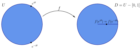
Figure 1. An example of a univalent function in $U$ for which $K\left(f,U\right)=0$.

The main result is contained in the following:

Theorem 2.4.

Let $f:D\rightarrow\mathbb{C}$ be a non-constant analytic function in the convex domain $D$. If there exists an analytic function $g:D\rightarrow\mathbb{C}$ univalent in $D$ such that

(2.2) $$\left|f^{\prime}\left(z\right)-g^{\prime}\left(z\right)\right|\leq K\left(g,D\right),\qquad z\in D,$$

then the function $f$ is also univalent in $D$.

Proof.

Assuming that $f$ is not univalent in $D$, there exists distinct points $z_{1,2}\in D$ such that $f\left(z_{1}\right)=f\left(z_{2}\right)$. Integrating the derivative of $f-g$ along the line segment $\left[z_{1},z_{2}\right]\subset D$ and using the hypothesis (2.2) we obtain

$$\left|g\left(z_{2}\right)-g\left(z_{1}\right)\right| = \left|\left(f\left(z_{2}\right)-g\left(z_{2}\right)\right)-\left(f\left(z_{1}\right)-g\left(z_{1}\right)\right)\right|$$

$$= \left|\int_{\left[z_{1},z_{2}\right]}f^{\prime}\left(z\right)-g^{\prime}\left(z\right)dz\right|$$

$$\leq \int_{\left[z_{1},z_{2}\right]}\left|f^{\prime}\left(z\right)-g^{\prime}\left(z\right)\right|\left|dz\right|$$

$$\leq \int_{\left[z_{1},z_{2}\right]}K\left(g,D\right)\left|dz\right|$$

$$= K\left(g,D\right)\left|z_{1}-z_{2}\right|.$$

Since the points $z_{1,2}$ are assumed to be distinct, from the definition of the constant $K\left(g,D\right)$ we obtain equivalently

(2.3) $$\left|\frac{g\left(z_{2}\right)-g\left(z_{1}\right)}{z_{2}-z_{1}}\right|\leq K\left(g,D\right)=\inf_{\begin{subarray}{c}a,b\in D\\ a\neq b\end{subarray}}\left|\frac{g\left(a\right)-g\left(b\right)}{a-b}\right|\leq\left|\frac{g\left(z_{2}\right)-g\left(z_{1}\right)}{z_{2}-z_{1}}\right|,$$

and therefore

(2.4) $$K\left(g,D\right)=\inf_{\begin{subarray}{c}a,b\in D\\ a\neq b\end{subarray}}\left|\frac{g\left(a\right)-g\left(b\right)}{a-b}\right|=\left|\frac{g\left(z_{2}\right)-g\left(z_{1}\right)}{z_{2}-z_{1}}\right|.$$

Consider now the auxiliary function $G:D-\left\{z_{2}\right\}\rightarrow\mathbb{C}$ defined by

(2.5) $$G\left(z\right)=\frac{g\left(z\right)-g\left(z_{2}\right)}{z-z_{2}},\qquad z\in D-\left\{z_{2}\right\},$$

and note that since $g$ is analytic in $D$, $G$ is also analytic in $D-\left\{z_{2}\right\}$ and moreover the limit

(2.6) $$\lim_{z\rightarrow z_{2}}G\left(z\right)=\lim_{z\rightarrow z_{2}}\frac{g\left(z\right)-g\left(z_{2}\right)}{z-z_{2}}=g^{\prime}\left(z_{2}\right)$$

exists and it is finite. The function $G$ can be therefore extended by continuity to an analytic function in $D$, denoted also by $G$.

Since

$$\inf_{z\in D}\left|G\left(z\right)\right|=\inf_{\begin{subarray}{c}z\in D\\ z\neq z_{2}\end{subarray}}\left|G\left(z\right)\right|=\inf_{\begin{subarray}{c}z\in D\\ z\neq z_{2}\end{subarray}}\left|\frac{g\left(z\right)-g\left(z_{2}\right)}{z-z_{2}}\right|\geq\inf_{\begin{subarray}{c}a,b\in D\\ a\neq b\end{subarray}}\left|\frac{g\left(a\right)-g\left(b\right)}{a-b}\right|=K\left(g,D\right),$$

combining with (2.4) we obtain that

$$\inf_{z\in D}\left|G\left(z\right)\right|\geq K\left(g,D\right)=\left|\frac{g\left(z_{2}\right)-g\left(z_{1}\right)}{z_{2}-z_{1}}\right|=\left|G\left(z_{1}\right)\right|\geq\inf_{z\in D}\left|G\left(z\right)\right|,$$

which shows that minimum value of the modulus of $G$ in $D$ is attained at $z_{1}$:

$$\inf_{z\in D}\left|G\left(z\right)\right|=\left|G\left(z_{1}\right)\right|.$$

However, since the function $g$ is univalent in $D$, from the definition of $G$ it follows that $G\left(z\right)\neq 0$ for any $z\in D-\left\{z_{2}\right\}$, and also $G\left(z_{2}\right)=g^{\prime}\left(z_{2}\right)\neq 0$, and therefore the function $G$ does not vanish in $D$. Applying the maximum modulus principle to the analytic function $1/G$ it follows that $\left|G\right|$ must be constant in $D$, and therefore $G$ is constant in $D$.

It follows that

(2.7) $$g\left(z\right)=g\left(z_{2}\right)+c\left(z-z_{2}\right),\qquad z\in D,$$

for a certain constant $c\in\mathbb{C}$ (from the definition of $G$ it can be seen that the constant $c$ can be written in the form $c=g^{\prime}\left(z_{2}\right)e^{i\theta}$, for some $\theta\in\mathbb{R}$).

The relation (2.7) shows that $g$ is a linear function, and therefore the constant $K\left(g,D\right)$ becomes in this case

$$K\left(g,D\right) = \inf_{\begin{subarray}{c}a,b\in D\\ a\neq b\end{subarray}}\left|\frac{g\left(a\right)-g\left(b\right)}{a-b}\right|$$

$$= \inf_{\begin{subarray}{c}a,b\in D\\ a\neq b\end{subarray}}\left|\frac{\left(g\left(z_{2}\right)+c\left(a-z_{2}\right)\right)-\left(g\left(z_{2}\right)+c\left(b-z_{2}\right)\right)}{a-b}\right|$$

$$= \inf_{\begin{subarray}{c}a,b\in D\\ a\neq b\end{subarray}}\left|\frac{c\left(a-b\right)}{a-b}\right|$$

$$= \left|c\right|.$$

The hypothesis (2.2) of the theorem can be written therefore as follows

$$\left|f^{\prime}\left(z\right)-c\right|\leq\left|c\right|,\qquad z\in D,$$

which shows that either $f$ is linear in $D$ (and thus univalent, since $f$ is assumed to be non-constant in $D$), or the following strict inequality holds

$$\left|f^{\prime}\left(z\right)-c\right|<\left|c\right|,\qquad z\in D.$$

Repeating the proof above with $g\left(z\right)\equiv cz$ we obtain

$$\left|cz_{2}-cz_{1}\right| = \left|\left(f\left(z_{2}\right)-cz_{2}\right)-\left(f\left(z_{1}\right)-cz_{1}\right)\right|$$

$$= \left|\int_{\left[z_{1},z_{2}\right]}f^{\prime}\left(z\right)-cdz\right|$$

$$\leq \int_{\left[z_{1},z_{2}\right]}\left|f^{\prime}\left(z\right)-c\right|\left|dz\right|$$

$$< \left|c\right|\left|z_{2}-z_{1}\right|,$$

a contradiction.

The contradiction obtained shows that the function $f$ is univalent in $D$, concluding the proof of the theorem. ∎

In the particular case $D=U$, from the previous thereom we obtain immediately the following sufficient criterion for univalence in the unit disk:

Theorem 2.5.

Let $f:U\rightarrow\mathbb{C}$ be a non-constant analytic function in the unit disk. If there exists an analytic function $g:U\rightarrow\mathbb{C}$ univalent in $U$ such that

(2.8) $$\left|f^{\prime}\left(z\right)-g^{\prime}\left(z\right)\right|\leq K\left(g,U\right),\qquad z\in U,$$

then the function $f$ is also univalent in $U$.

As a corollary of Theorem 2.4 we obtain immediately the following:

Corollary 2.6.

If $f:D\rightarrow\mathbb{C}$ is non-constant and analytic in the convex domain $D$ and there exists $c>0$ such that

(2.9) $$\left|f^{\prime}\left(z\right)-c\right|\leq c,\qquad z\in D,$$

then $f$ is univalent in $D$.

Proof.

Considering the univalent function $g:D\rightarrow\mathbb{C}$ defined by $g\left(z\right)=cz$, we have $g^{\prime}\left(z\right)=c$ for $z\in D$ and

$$K\left(g,D\right)=\inf_{\begin{subarray}{c}a,b\in D\\ a\neq b\end{subarray}}\left|\frac{g\left(a\right)-g\left(b\right)}{a-b}\right|=\inf_{\begin{subarray}{c}a,b\in D\\ a\neq b\end{subarray}}\left|\frac{ca-cb}{a-b}\right|=c,$$

and therefore the claim follows from Theorem 2.4 above. ∎

Remark 2.7.

Let us note that the previous corollary can also be obtained as a direct consequence of the classical Noshiro-Warschawski-Wolff univalence criterion, since the hypothesis (2.9) implies the hypothesis

(2.10) $$\mathop{\rm Re}\nolimits f^{\prime}\left(z\right)>0,\qquad z\in D.$$

of this theorem (the fact that the above inequality is a strict inequality follows from the maximum principle, the function $f$ being assumed to be non-constant in $D$).

Conversely, the Noshiro-Warschawski-Wolff univalence criterion follows from the previous corollary. To see this, note that in order to prove the univalence of $f$, it suffices to prove the univalence of $f$ in $D_{r}=rD$, for an arbitrarily fixed $r\in(0,1)$.

If the condition (2.10) holds, there exists $c>0$ such that

$$f^{\prime}\left(D_{r}\right)\subset\left\{w\in\mathbb{C}:\left|w-c\right|<c\right\},$$

or equivalent

$$\left|f^{\prime}\left(z\right)-c\right|<c,\qquad z\in D_{r}.$$

Applying Corollary 2.6 to the restriction of of $f$ to $D_{r}$, it follows that the function $f$ is univalent in $D_{r}.$ Since $r\in\left(0,1\right)$ was arbitrarily fixed, it follows that $f$ is univalent in $U$, concluding the proof of the claim.

The remark above shows that Corollary 2.6 and the Noshiro-Warschawski-Wolff univalence criterion are equivalent, and therefore Theorem 2.4 is a generalization of it. The Noshiro-Warschawski-Wolff univalence criterion can be viewed as a particular case of the main Theorem 2.4, corresponding to the choice of a linear function $g$.

Remark 2.8.

Fixing an arbitrarily univalent function $g:U\rightarrow\mathbb{C}$ for which $K\left(g,U\right)\neq 0$ (see Remark 2.2 above), Theorem 2.5 shows that a whole neighborhood $V\left(g\right)=\left\{f\in\mathcal{A}:\left|\left|f^{\prime}-g^{\prime}\right|\right|\leq K\left(g,U\right)\right\}$ of $g$ consists entirely of univalent functions in $U$ ($\left|\left|\cdot\right|\right|$ denotes here the supremum norm in the space $\mathcal{A}_{0}=\left\{f\in\mathcal{A}:f\left(0\right)=0\right\}$ of normalized analytic functions). Loosely stated, Theorem 2.5 shows that an univalent function has a neighborhood consisting entirely of univalent functions.

The hypotheses of Theorem 2.4 and Theorem 2.5 are sharp, in the sense that we cannot replace the right side of the inequalities (2.2), respectively (2.8), by larger constants, as can be seen from the following example.

Example 2.9.

Consider the function $f:U\rightarrow\mathbb{C}$ defined by $f\left(z\right)=z+az^{2}$, $z\in U$, where $a\in\mathbb{C}$ is a parameter.

Using Theorem 2.5 above with $g\left(z\right)\equiv z$, for which $K\left(g,U\right)=1$, we obtain that the function $f$ is univalent in $U$ if

$$\left|2az\right|\leq 1,\qquad z\in U,$$

that is if $\left|2a\right|\leq 1$.

This result is sharp, since the function $f$ is univalent iff $\left|a\right|\leq\frac{1}{2}$, as it can be checked by direct computation.

The univalence of the function $f$ in the previous example can also be obtained by using the Noshiro-Warschawski-Wolff univalence criterion (for $\left|a\right|\leq 1/2$ we have $\mathop{\rm Re}\nolimits f^{\prime}\left(z\right)>0$ for any $z\in U$). The next example shows that we may still use Theorem 2.5 also in situations when the Noshiro-Warschawski-Wolff univalence criterion cannot be applied:

Example 2.10.

Consider the linear map $g:U\rightarrow\mathbb{C}$ defined by $g\left(z\right)=\frac{z}{1-z}$. The function $g$ is univalent in $U$ and we have

$$K\left(g,U\right)=\inf_{\begin{subarray}{c}a,b\in U\\ a\neq b\end{subarray}}\left|\frac{g\left(a\right)-g\left(b\right)}{a-b}\right|=\inf_{\begin{subarray}{c}a,b\in U\\ a\neq b\end{subarray}}\left|\frac{\frac{a}{1-a}-\frac{b}{1-b}}{a-b}\right|=\inf_{\begin{subarray}{c}a,b\in U\\ a\neq b\end{subarray}}\frac{1}{\left|1-a\right|\left|1-b\right|}=1.$$

The function $f:U\rightarrow\mathbb{C}$ defined by $f\left(z\right)=\frac{z^{2}}{1-z}$ is analytic in $U$ and satisfies

$$\left|f^{\prime}\left(z\right)-g^{\prime}\left(z\right)\right|=1\leq K\left(g,U\right),\qquad z\in U,$$

and therefore by Theorem 2.5 it follows that $f$ is univalent in the unit disk.

The univalence of $f$ does not follow however by the Noshiro-Warschawski-Wolff univalence criterion since $\mathop{\rm Re}\nolimits f^{\prime}\left(z\right)$ takes (arbitrarily small) negative values for $z\in U$ sufficiently close to $1$.

As another application of Theorem 2.5, in the next result we show that by perturbing the coefficients of the Taylor series of an univalent function, the resulting function is also univalent. More precisely, we have the following:

Theorem 2.11.

Let $g:U\rightarrow\mathbb{C}$ be an analytic univalent function with Taylor series representation

(2.11) $$g\left(z\right)=\sum_{n=0}^{\infty}b_{n}z^{n},\qquad z\in U\text{.}$$

If the coefficients $a_{0},a_{1},\ldots\in\mathbb{C}$ satisfy the inequality

(2.12) $$\sum_{n=1}^{\infty}n\left|a_{n}-b_{n}\right|<K\left(g,U\right)$$

then the function $f:U\rightarrow\mathbb{C}$ defined by

(2.13) $$f\left(z\right)=\sum_{n=0}^{\infty}a_{n}z^{n},\qquad z\in U,$$

is analytic and univalent in $U$.

Proof.

Since $g$ is univalent in $U$, the radius of convergence of the Taylor series (2.11) is at least $1$, hence

$$\lim\sup\sqrt[n]{\left|b_{n}\right|}\leq 1,$$

and therefore $\left|b_{n}\right|\leq 1$ for all $n$ sufficiently large.

Using the hypothesis (2.12) we obtain

$$\lim\sup\sqrt[n]{\left|a_{n}\right|}\leq\lim\sup\sqrt[n]{\left|b_{n}\right|+\left|a_{n}-b_{n}\right|}\leq\lim\sup\sqrt[n]{1+\frac{K\left(g,U\right)}{n}}=1,$$

and therefore the radius of convergence of the series in (2.13) is at least $1$, thus the function $f$ is well defined by (2.13) and it is analytic in $U$.

Since

$$\left|f^{\prime}\left(z\right)-g^{\prime}\left(z\right)\right| = \left|\sum_{n=0}^{\infty}na_{n}z^{n-1}-\sum_{n=0}^{\infty}nb_{n}z^{n-1}\right|$$

$$\leq \sum_{n=1}^{\infty}n\left|a_{n}-b_{n}\right|\left|z\right|^{n-1}$$

$$\leq \sum_{n=1}^{\infty}n\left|a_{n}-b_{n}\right|$$

$$< K\left(g,U\right),$$

for any $z\in U$, by Theorem 2.5 follows that $f$ is univalent in $U$, concluding the proof. ∎

Using a comparison with the generalized harmonic series, from the above we can obtain the following:

Corollary 2.12.

Let $g:U\rightarrow\mathbb{C}$ be an analytic univalent function with Taylor series representation

(2.14) $$g\left(z\right)=\sum_{n=0}^{\infty}b_{n}z^{n},\qquad z\in U\text{.}$$

If the coefficients $a_{0},a_{1},\ldots\in\mathbb{C}$ satisfy the inequality

(2.15) $$\left|a_{n}-b_{n}\right|<K\left(g,U\right)\frac{\zeta\left(p\right)}{n^{p+1}},\qquad n=1,2,\ldots,$$

for some $p>1$ ($\zeta$ denotes the Riemann zeta function), then the function $f:U\rightarrow\mathbb{C}$ defined by

(2.16) $$f\left(z\right)=\sum_{n=0}^{\infty}a_{n}z^{n},\qquad z\in U,$$

is analytic and univalent in $U$.

Example 2.13.

Considering the function $g\left(z\right)=\frac{z}{1-z}=\sum_{n=1}^{\infty}z^{n}$ defined in Example 2.10, which is analytic and univalent in $U$ and has $K\left(g,U\right)=1$, from the previous theorem it follows that the function $f:U\rightarrow\mathbb{C}$ defined by $f\left(z\right)=\sum_{n=0}^{\infty}a_{n}z^{n}$ is analytic and univalent in $U$ if the coefficients $a_{n}$ satisfy the inequality

$$\sum_{n=1}^{\infty}n\left|a_{n}-1\right|<1.$$

Using for example the fact that $\zeta\left(2\right)=\frac{\pi^{2}}{6}\approx 1.645$, from the previous corollary it follows that the function $f$ is also analytic and univalent in $U$ if the coefficients $a_{n}$ satisfy the inequality

$$\left|a_{n}-1\right|\leq\frac{\pi^{2}}{6n^{3}}\approx\frac{1.645}{n^{3}},\qquad n=1,2,\ldots$$

References

- [1] Ch. Pommerenke, Boundary behaviour of conformal maps, Springer-Verlag, Berlin, 1992.