Energy gaps at neutrality point … Energy gaps at neutrality point in bilayer graphene in a magnetic field E. V. Gorbar, V. P. Gusynin, V. A.  Miransky Gorbar,Gusynin,Miransky 15 January 2010*

Energy gaps at neutrality point in bilayer graphene in a magnetic field

Abstract

Utilizing the Baym-Kadanoff formalism with the polarization function calculated in the random phase approximation, the dynamics of the $\nu=0$ quantum Hall state in bilayer graphene is analyzed. Two phases with nonzero energy gap, the ferromagnetic and layer asymmetric ones, are found. The phase diagram in the plane $(\tilde{\Delta}_{0},B)$, where $\tilde{\Delta}_{0}$ is a top-bottom gates voltage imbalance, is described. It is shown that the energy gap scales linearly, $\Delta E\sim 14B[{\mbox{T}}]{\mbox{K}}$, with magnetic field.

81.05.ue, 73.43.-f, 73.43.Cd

Introduction.— The possibility of inducing and controlling the energy gap by gates voltage makes bilayer graphene [1, 2, 3] one of the most active research areas with very promising applications in electronic devices. Recent experiments in bilayer graphene [4, 5] showed the generation of gaps in a magnetic field with complete lifting of the eight-fold degeneracy in the zero energy Landau level, which leads to new quantum Hall states with filling factors $\nu=0,\pm 1,\pm 2,\pm 3$. Besides that, in suspended bilayer graphene, Ref.[4] reports the observation of an extremely large magnetoresistance in the $\nu=0$ state due to the energy gap $\Delta E$, which scales linearly with a magnetic field $B$, $\Delta E\sim 3.5-10.5B[{\mbox{T}}]{\mbox{K}}$, for $B\lesssim 10{\mbox{T}}$. This linear scaling is hard to explain by the standard mechanisms [6, 7] of gap generation used in a monolayer graphene, which lead to large gaps of the order of the Coulomb energy $e^{2}/l\sim B^{1/2}$, $l=(\hbar c/eB)^{1/2}$ is the magnetic length.

In this Letter, we study the dynamics of clean bilayer graphene in a magnetic field, with the emphasis on the $\nu=0$ state in the quantum Hall effect (QHE). It will be shown that, as in the case of monolayer graphene [8], the dynamics in the QHE in bilayer graphene is described by the coexisting quantum Hall ferromagnetism (QHF) [6] and magnetic catalysis (MC)[7] order parameters. The essence of the dynamics is an effective reduction by two units of the spatial dimension in the electron-hole pairing in the lowest Landau level (LLL) with energy $E=0$ [9, 10, 11]. As we discuss below, there is however an essential difference between the QHE’s in these two systems. While the pairing forces in monolayer graphene lead to a relativistic-like scaling $\Delta E\sim\sqrt{|eB|}$ for the dynamical gap, in bilayer graphene, such a scaling takes place only for strong magnetic fields, $B\gtrsim B_{thr}$, where our estimate yields $B_{thr}\sim 30-60{\mbox{T}}$. For $B\lesssim B_{thr}$, a nonrelativistic-like scaling $\Delta E\sim|eB|$ is realized in the bilayer. The origin of this phenomenon is very different forms of the polarization function in monolayer graphene and bilayer one that in turn is determined by the different dispersion relations for quasiparticles in these two systems. The polarization function is one of the major players in the QHE in bilayer, and its consideration distinguishes this work from the most of previous theoretical ones studying the QHE in bilayer graphene [12] .

Using the random phase approximation in the analysis of the gap equation, we found that the gap in the clean bilayer is $\Delta E\sim 14B[{\mbox{T}}]{\mbox{K}}$ for the magnetic field $B\lesssim B_{thr}$. The phase diagram in the plane $(\tilde{\Delta}_{0},B)$, where $\tilde{\Delta}_{0}$ is a top-bottom gates voltage imbalance, is described. These are the central results of this Letter.

Hamiltonian.— The free part of the effective low energy Hamiltonian of bilayer graphene is [1]:

$$H_{0}=-\frac{1}{2m}\int d^{2}x\Psi_{Vs}^{+}(x)\left(\begin{array}[]{cc}0&(\pi^{\dagger})^{2}\\ \pi^{2}&0\end{array}\right)\Psi_{Vs}(x),$$ (1)

where $\pi=\hat{p}_{x_{1}}+i\hat{p}_{x_{2}}$ and the canonical momentum $\hat{\mathbf{p}}=-i\hbar\bm{\nabla}+{e\mathbf{A}}/c$ includes the vector potential $\mathbf{A}$ corresponding to the external magnetic field $\mathbf{B}$. Without magnetic field, this Hamiltonian generates the spectrum $E=\pm\frac{p^{2}}{2m}$, $m=\gamma_{1}/2v_{F}^{2}$, where the Fermi velocity $v_{F}\simeq c/300$ and $\gamma_{1}\approx 0.34-0.40$eV. The two component spinor field $\Psi_{Vs}$ carries the valley $(V=K,K^{\prime})$ and spin $(s=+,-)$ indices. We will use the standard convention: $\Psi_{Ks}^{T}=(\psi_{A}{{}_{1}},\psi_{B}{{}_{2}})_{Ks}$ whereas $\Psi_{K^{\prime}s}^{T}=(\psi_{B}{{}_{2}},\psi_{A}{{}_{1}})_{K^{\prime}s}$. Here $A_{1}$ and $B_{2}$ correspond to those sublattices in the layers 1 and 2, respectively, which, according to Bernal $(A_{2}-B_{1})$ stacking, are relevant for the low energy dynamics. The effective Hamiltonian (1) is valid for magnetic fields $1T<B<B_{thr}$. For $B<1T$, the trigonal warping should be taken into account [1]. For $B>B_{thr}$, a monolayer like Hamiltonian with linear dispersion should be used.

The Zeeman and Coulomb interactions in bilayer graphene are (henceforth we will omit indices $V$ and $s$ in the field $\Psi_{Vs}$):

$$H_{int}=\mu_{B}B\int d^{2}x\Psi^{+}(x)\sigma^{3}\Psi(x)+\frac{e^{2}}{2\kappa}\int d^{3}xd^{3}x^{\prime}\frac{n(\mathbf{x})n(\mathbf{x}^{\prime})}{|\mathbf{x}-\mathbf{x}^{\prime}|}$$

$$=\mu_{B}B\int d^{2}x\Psi^{+}(x)\sigma^{3}\Psi(x)+\frac{1}{2}\int d^{2}xd^{2}x^{\prime}\left[V(x-x^{\prime})\right.$$

$$\left.\times\left(\rho_{1}(x)\rho_{1}(x^{\prime})+\rho_{2}(x)\rho_{2}(x^{\prime})\right)+2V_{12}(x-x^{\prime})\rho_{1}(x)\rho_{2}(x^{\prime})\right],$$

(2)

where $\mu_{B}$ is the Bohr magneton, $\kappa$ is the dielectric constant, and $n(\mathbf{x})=\delta(z-\frac{d}{2})\rho_{1}(x)+\delta(z+\frac{d}{2})\rho_{2}(x)$ is the three dimensional charge density ($d\simeq 0.3$nm is the distance between the two layers). The interaction potentials $V(x)$ and $V_{12}(x)$ describe the intralayer and interlayer interactions, respectively. Their Fourier transforms are ${V}(k)=2\pi e^{2}/\kappa k$ and ${V}_{12}(k)=2\pi e^{2}e^{-kd}/\kappa k$. The two-dimensional charge densities $\rho_{1}(x)$ and $\rho_{2}(x)$ are:

$$\rho_{1}(x)=\Psi^{+}(x)P_{1}\Psi(x)\,,\quad\rho_{2}(x)=\Psi^{+}(x)P_{2}\Psi(x)\,,$$ (3)

where $P_{1}=\frac{1+\xi\tau^{3}}{2}$ and $P_{2}=\frac{1-\xi\tau^{3}}{2}$ are projectors on states in the layers 1 and 2, respectively [here $\tau^{3}$ is the Pauli matrix acting on layer components, and $\xi=\pm 1$ for the valleys $K$ and $K^{\prime}$, respectively].

Symmetries.— The Hamiltonian $H=H_{0}+H_{int}$ describes the dynamics at the neutral point (with no doping). Because of the projectors $P_{1}$ and $P_{2}$ in charge densities (3), the symmetry of the Hamiltonian $H$ is essentially lower than the symmetry in monolayer graphene. If the Zeeman term is ignored, it is $U^{(K)}(2)_{S}\times U^{(K^{\prime})}(2)_{S}\times Z_{2V}^{(+)}\times Z_{2V}^{(-)}$, where $U^{(V)}(2)_{S}$ defines the $U(2)$ spin transformations in a fixed valley $V=K,K^{\prime}$, and $Z_{2V}^{(s)}$ describes the valley transformation $\xi\to-\xi$ for a fixed spin $s=\pm$ (recall that in monolayer graphene the symmetry would be $U(4)$ [11]). The Zeeman interaction lowers this symmetry down to $G_{2}\equiv U^{(K)}(1)_{+}\times U^{(K)}(1)_{-}\times U^{(K^{\prime)}}(1)_{+}\times U^{(K^{\prime)}}(1)_{-}\times Z_{2V}^{(+)}\times Z_{2V}^{(-)}$, where $U^{(V)}(1)_{s}$ is the $U(1)$ transformation for fixed values of both valley and spin. Recall that the corresponding symmetry in monolayer graphene is $G_{1}\equiv U^{(+)}(2)_{V}\times U^{(-)}(2)_{V}$, where $U^{(s)}(2)_{V}$ is the $U(2)$ valley transformations for a fixed spin.

Order parameters.— Although the $G_{1}$ and $G_{2}$ symmetries are quite different, it is noticeable that their breakdowns can be described by the same QHF and MC order parameters. The point is that these $G_{1}$ and $G_{2}$ define the same four conserved commuting currents whose charge densities (and four corresponding chemical potentials) span the QHF order parameters (we use the notations of Ref. [8]):

$$\mu_{s}:\quad\Psi^{\dagger}_{s}\Psi_{s} = \psi_{KA_{1}s}^{\dagger}\psi_{KA_{1}s}+\psi_{K^{\prime}A_{1}s}^{\dagger}\psi_{K^{\prime}A_{1}s}$$ (4)

$$+ \psi_{KB_{2}s}^{\dagger}\psi_{KB_{2}s}+\psi_{K^{\prime}B_{2}s}^{\dagger}\psi_{K^{\prime}B_{2}s}\,,$$

$$\tilde{\mu}_{s}:\quad\Psi^{\dagger}_{s}\xi\Psi_{s} = \psi_{KA_{1}s}^{\dagger}\psi_{KA_{1}s}-\psi_{K^{\prime}A_{1}s}^{\dagger}\psi_{K^{\prime}A_{1}s}$$ (5)

$$+ \psi_{KB_{2}s}^{\dagger}\psi_{KB_{2}s}-\psi_{K^{\prime}B_{2}s}^{\dagger}\psi_{K^{\prime}B_{2}s}\,.$$

The order parameter (4) is the charge density for a fixed spin whereas the order parameter (5) determines the charge-density imbalance between the two valleys. The corresponding chemical potentials are $\mu_{s}$ and $\tilde{\mu}_{s}$, respectively. While the former order parameter preserves the $G_{2}$ symmetry, the latter completely breaks its discrete subgroup $Z_{2V}^{(s)}$. Their MC cousins are

$$\Delta_{s}:\quad\Psi^{\dagger}_{s}\tau_{3}\Psi_{s} = \psi_{KA_{1}s}^{\dagger}\psi_{KA_{1}s}-\psi_{K^{\prime}A_{1}s}^{\dagger}\psi_{K^{\prime}A_{1}s}$$ (6)

$$- \psi_{KB_{2}s}^{\dagger}\psi_{KB_{2}s}+\psi_{K^{\prime}B_{2}s}^{\dagger}\psi_{K^{\prime}B_{2}s}\,,$$

$$\tilde{\Delta}_{s}:\quad\Psi^{\dagger}_{s}\xi\tau_{3}\Psi_{s} = \psi_{KA_{1}s}^{\dagger}\psi_{KA_{1}s}+\psi_{K^{\prime}A_{1}s}^{\dagger}\psi_{K^{\prime}A_{1}s}$$ (7)

$$- \psi_{KB_{2}s}^{\dagger}\psi_{KB_{2}s}-\psi_{K^{\prime}B_{2}s}^{\dagger}\psi_{K^{\prime}B_{2}s}\,.$$

These order parameters can be rewritten in the form of Dirac mass terms [8] corresponding to the masses $\Delta_{s}$ and $\tilde{\Delta}_{s}$, respectively. While the order parameter (6) preserves the $G_{2}$, it is odd under time reversal $\cal{T}$ [14]. On the other hand, the order parameter (7) is connected with the conventional Dirac mass $\tilde{\Delta}$. It determines the charge-density imbalance between the two layers [1]. Like $\tilde{\mu}_{s}$, this mass term completely breaks the $Z_{2V}^{(s)}$ symmetry and is even under $\cal{T}$. Note that because of the Zeeman interaction, the $SU^{(V)}(2)_{S}$ is explicitly broken, leading to a spin gap. This gap could be dynamically strongly enhanced [15]. In that case, a quasispontaneous breakdown of the $SU^{(V)}(2)_{S}$ takes place. The corresponding ferromagnetic phase is described by $\mu_{3}=(\mu_{+}-\mu_{-})/2$ with the QHF order parameter $\Psi^{\dagger}\sigma_{3}\Psi$, and by $\Delta_{3}=(\Delta_{+}-\Delta_{-})/2$ with the MC order parameter $\Psi^{\dagger}\tau_{3}\sigma_{3}\Psi$ [8].

Gap equation.— In the framework of the Baym-Kadanoff formalism [16], and using the polarization function calculated in the random phase approximation (RPA), we analyzed the gap equation for the LLL quasiparticle propagator with the order parameters introduced above. Recall that in bilayer graphene, the LLL includes both the $n=0$ and $n=1$ LLs, if the Coulomb interaction is ignored [1]. Therefore there are sixteen parameters $\mu_{s}(n)$, $\Delta_{s}(n)$, $\tilde{\mu}_{s}(n)$, and $\tilde{\Delta}_{s}(n)$, where the index $n=0,1$ corresponds to the $n=0$ and $n=1$ LLs, respectively. The following system of equations was derived for these parameters:

$$G^{-1}_{\xi s0}(\Omega) = S^{-1}_{\xi s}(\Omega)-i\int\frac{d\omega\,d^{2}k}{(2\pi)^{3}}\,e^{-\mathbf{k}^{2}l^{2}/2}[G_{\xi s0}(\omega)$$ (8)

$$+ G_{\xi s1}(\omega)\mathbf{k}^{2}l^{2}/2]{V}_{eff}\left(\Omega-\omega,|\mathbf{k}|\right)$$

$$- \frac{e^{2}d}{2\kappa l^{2}}\,\left(\frac{1+\xi}{2}A_{1}+\frac{1-\xi}{2}A_{2}\,\right),$$

$$G^{-1}_{\xi s1}(\Omega) = S^{-1}_{\xi s}(\Omega)-i\int\frac{d\omega\,d^{2}k}{(2\pi)^{3}}\,e^{-\mathbf{k}^{2}l^{2}/2}[G_{\xi s0}(\omega)$$ (9)

$$\times \mathbf{k}^{2}l^{2}/2+G_{\xi s1}(\omega)(1-\mathbf{k}^{2}l^{2}/2)^{2}]$$

$$\times V_{eff}\left(\Omega-\omega,|\mathbf{k}|\right)$$

$$- \frac{e^{2}d}{2\kappa l^{2}}\,\left(\frac{1+\xi}{2}A_{1}+\frac{1-\xi}{2}A_{2}\right)\,.$$

Here $A_{1}=\sum_{n,s}\,\mbox{sgn}(\,E_{-ns})$ , $A_{2}=\sum_{n,s}\,\mbox{sgn}(\,E_{+ns})$, and

$$S_{\xi s}(\omega)=\frac{1}{\omega+\mu_{0}-sZ+\xi\tilde{\Delta}_{0}},\,G_{\xi sn}(\omega)=\frac{1}{\omega-E_{\xi ns}}$$ (10)

are frequency dependent factors in the bare and full LLL propagators, where

$$E_{\xi ns}=-(\mu_{s}(n)+\Delta_{s}(n))+\xi(\tilde{\mu}_{s}(n)-\tilde{\Delta}_{s}(n))$$ (11)

are the energies of the LLL states, $\mu_{0}$ is chemical potential, $Z$ is the Zeeman energy, $Z\simeq\mu_{B}B=0.67\,B[{\mbox{T}}]{\mbox{K}}$. The second and third terms on right hand sides of Eqs.(8), (9) describe the Fock and Hartree interactions, respectively. Note that because for the LLL states only the component $\psi_{B_{2}s}$ $(\psi_{A_{1}s})$ of the wave function at the $K(K^{\prime})$ valley is nonzero, their energies depend only on the eight independent combinations of the QHF and MC parameters shown in Eq.(11). The function ${V}_{eff}(\omega,k)$, describing the Coulomb interaction, is

$${V}_{eff}(\omega,k)=\frac{2\pi e^{2}}{\kappa}\,\frac{1}{k+\frac{4\pi e^{2}}{\kappa}\Pi(\omega,{\bf k}^{2})},$$ (12)

where $\Pi(\omega,{\bf k}^{2})$ is the polarization function in a magnetic field. Since the dependence of $\Pi(\omega,{\bf k}^{2})$ on $\omega$ is weak, the static polarization will be used. Then, in the case of frequency independent order parameters, the integration over $\omega$ in Eqs. (8), (9) can be performed explicitly, and we get a system of algebraic equations for the energies $E_{\xi ns}$ of the LLL states.

It is convenient to rewrite the static polarization $\Pi(0,{\bf k}^{2})$ in the form $\Pi=(m/{\hbar}^{2})\tilde{\Pi}(y)$, where both $\tilde{\Pi}$ and $y\equiv\mathbf{k}^{2}l^{2}/2$ are dimensionless. The function $\tilde{\Pi}(y)$ was expressed in terms of the sum over all the Landau levels and was analyzed both analytically and numerically. At $y\ll 1$, it behaves as $\tilde{\Pi}(y)\simeq 0.55y$ and its derivative $\tilde{\Pi}^{\prime}$ changes from $0.55$ at $y=0$ to 0.12 at $y=1$. At large $y$, it approaches a zero magnetic field value, $\tilde{\Pi}(y)\simeq\ln 4/\pi$ (see Fig.1) .

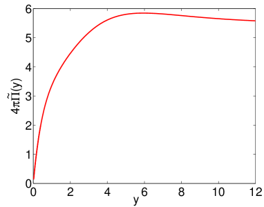
Figure 1: Fig. 1. The static polarization function $4\pi\tilde{\Pi}(y)$.

Because of the Gaussian factors $e^{-\mathbf{k}^{2}l^{2}/2}=e^{-y}$ in Eqs. (8) and (9), the relevant region in the integrals in these equations is $0<y\lesssim 1$. The crucial point in the analysis is that the region where the bare Coulomb term $k$ in the denominator of ${V}_{eff}(k)\equiv{V}_{eff}(0,k)$ (12) dominates is very small, $0<y\lesssim 10^{-3}B$[T]. The main reason of that is a large mass $m$ of quasiparticles, $m\sim 10^{-2}m_{e}\sim 10^{8}{\mbox{K}/c^{2}}$. As a result, the polarization function term dominates in ${V}_{eff}(k)$ that leads to ${V}_{eff}(k)=C(y)\hbar^{2}/ml^{2}k^{2}$, where the part with the factor $1/k^{2}$ corresponds to the Coulomb potential in two dimensions, and the function $C(y)$ describes its smooth modulations at $0\leq y\lesssim 1$ (see Fig.1). It is unlike the case of the monolayer graphene where the effective interaction is proportional to $1/k$. As we discuss below, this in turn implies that, in the low energy model described by the Hamiltonian in Eqs. (1), (2), the scaling $\Delta E\sim|eB|$ takes place for the dynamical energy gap, and not $\Delta E\sim\sqrt{|eB|}$ taking place in monolayer graphene [6, 7, 8].

Last but not least, using the model with four-component wave functions [1], we determined the upper limit for the values of $B$, $B_{thr}$, for which the low energy effective model can be used. We found that $B_{thr}\sim 30-60$T, corresponding to the experimental values $0.34-0.40$eV of the parameter $\gamma_{1}=2mv^{2}_{F}$. We predict that for the values $B>B_{thr}$, the monolayer like scaling, $\Delta E\sim\sqrt{|eB|}$, should take place.

Solutions.— At the neutral point ($\mu_{0}=0$, no doping), we found two competing solutions of Eqs. (8) and (9): I) a ferromagnetic (spin splitting) solution, and II) a layer asymmetric solution, actively discussed in the literature. The energy (11) of the LLL states of the solution I equals:

$$E^{(I)}_{\xi ns}=s(Z+\frac{I_{n}(B)}{2ml^{2}})-\xi\tilde{\Delta}_{0}\,,$$ (13)

where the notation $I_{n}(B)$ is used for the integrals

$$I_{0}(B)=\int\limits_{0}^{\infty}\frac{dy\,(1+y)e^{-y}}{\sqrt{xy}+4\pi\tilde{\Pi}(y)},I_{1}(B)=\int\limits_{0}^{\infty}\frac{dy\,(1-y+y^{2})e^{-y}}{\sqrt{xy}+4\pi\tilde{\Pi}(y)}$$ (14)

with $x=0.003B(T)$. Note that the Hartree interaction does not contribute to this solution. The situation is different for the solution II:

$$E^{(II)}_{\xi ns} = sZ-\xi(\tilde{\Delta}_{0}+\frac{I_{n}(B)}{2ml^{2}}-\frac{2e^{2}d}{\kappa l^{2}})\,.$$ (15)

The last term in the parenthesis is the Hartree one. For suspended bilayer graphene, we will take $\kappa=1$.

The energy density of the ground state for these solutions is ($a=I,II$):

$$\epsilon^{(a)}= - \frac{1}{8\pi l^{2}}\sum_{\xi=\pm}\sum_{s=\pm}\sum_{n=0,1}\left[|E_{\xi ns}^{(a)}|\right.$$ (16)

$$+ \left.(-s\,0.67B+\xi\tilde{\Delta}_{0})\,\mbox{sgn}\,E_{\xi ns}^{(a)}\right].$$

It is easy to check that for balanced bilayer ($\tilde{\Delta}_{0}=0$) the solution I is favorite. The main reason of this is the presence of the capacitor like Hartree contribution in the energy density of the solution II: it makes that solution less stable.

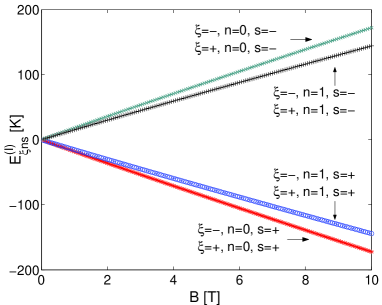
Figure 2: Fig. 2. The energies of the LLL states as functions of $B$.

For $\tilde{\Delta}_{0}=0$, the dependence of the LLL energies $E^{(I)}_{\xi ns}$ of the solution I on $B$ is shown in Fig. 2 (energy gaps are degenerate in $\xi$). The perfectly linear form of this dependence is evident. Also, the degeneracy between the states of the $n=0$ LL and those of the $n=1$ LL is removed. The energy gap corresponding to the $\nu=0$ plateau is $\Delta E=(E_{\xi 1-}^{(I)}-E_{\xi 1+}^{(I)})/2\simeq 14.3B[{\mbox{T}}]$K.

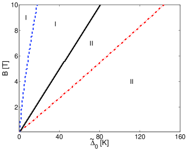
Figure 3: Fig. 3. The phase diagram in the $(\tilde{\Delta}_{0},B)$ plane.

In Fig. 3, the phase diagram in the plane $(\tilde{\Delta}_{0},B)$ is presented. The area marked by I (II) is that where the solution I (solution II) is favorite. The two dashed lines compose the boundary of the region where the two solutions coexist (the solution I does not exist to the right of the dashed line in the region II, while the solution II does not exist to the left of the dashed line in the region I). The bold line is the line of the first order phase transition. It is noticeable that for any fixed value of $B\,(\tilde{\Delta}_{0})$, there are sufficiently large values of $\tilde{\Delta}_{0}$  (B), at which the solution I (solution II) does not exist at all. It is because a voltage imbalance (Zeeman term) tends to destroy the solution I (solution II).

In conclusion, the dynamics of bilayer graphene in a magnetic field $B\lesssim B_{thr}$ is characterized by a very strong screening of the Coulomb interaction that relates to the presence of a large mass $m$ in the nonrelativistic-like dispersion relation for quasiparticles. The functional dependence of the gap on $B$ in Fig. 2 agrees with that obtained very recently in experiments in Ref. [4]. The existence of the first order phase transition in the plane $(\tilde{\Delta}_{0},B)$ is predicted. We also estimate the value $B_{thr}$, at which the change of the scaling $\Delta E\sim|eB|$ to $\Delta E\sim\sqrt{|eB|}$ occurs, as $B_{thr}\sim 30-60$T. It would be interesting to extend this analysis to the case of the higher, $\nu=1,2,$ and 3, LLL plateaus [4, 5].

We thank Junji Jia and S.G. Sharapov for fruitful discussions. The work of E.V.G and V.P.G. was supported partially by the SCOPES grant # IZ73Z0_128026 of the Swiss NSF, by the grant SIMTECH # 246937 of the European FP7 program, and by the grant RFFR-DFFD # 28.2/083. The work of V.A.M. was supported by the Natural Sciences and Engineering Research Council of Canada.

References

- [1] E. McCann and V. I. Fal’ko, Phys. Rev. Lett., 96, 086805, (2006); E. McCann, D. S. L. Abergel, and V. I. Fal’ko, Solid State Commun. 143, 110 (2007).
- [2] K. S. Novoselov et al, Nature Phys., 2, 177 (2006); E.A. Henriksen et al, Phys. Rev. Lett. 100, 087403 (2008).
- [3] A. H. Castro Neto et al., Rev. Mod. Phys. 81, 109 (2009).
- [4] B. E. Feldman, J. Martin, and A.Yacoby, Nature Phys. 5, 889 (2009).
- [5] Y. Zhao, P. Cadden-Zimansky, Z. Jiang, and P. Kim, Phys. Rev. Lett. 104, 066801 (2010).
- [6] K. Nomura and A.H. MacDonald, Phys. Rev. Lett. 96, 256602 (2006); K. Yang, S. Das Sarma, and A.H. MacDonald, Phys. Rev. B 74, 075423 (2006); M.O. Goerbig, R. Moessner, and B. Douçot, Phys. Rev. B 74, 161407(R) (2006); J. Alicea and M.P.A. Fisher, Phys. Rev. B 74, 075422 (2006); L. Sheng, D.N. Sheng, F.D.M. Haldane, and L. Balents, Phys. Rev. Lett. 99, 196802 (2007).
- [7] V.P. Gusynin, V.A. Miransky, S.G. Sharapov, and I.A. Shovkovy, Phys. Rev. B 74, 195429 (2006); I.F. Herbut, Phys. Rev. Lett. 97, 146401 (2006); Phys. Rev. B 75, 165411 (2007); J.-N. Fuchs and P. Lederer, Phys. Rev. Lett. 98, 016803 (2007); M. Ezawa, J. Phys. Soc. Jpn. 76 (2007) 094701.
- [8] E. V. Gorbar, V.P. Gusynin, and V. A. Miransky, Low Temp. Phys. 34, 790 (2008); E. V. Gorbar, V.P. Gusynin, V. A. Miransky, and I. A. Shovkovy, Phys. Rev. B 78, 085437 (2008).
- [9] V.P. Gusynin, V.A. Miransky, and I.A. Shovkovy, Phys. Rev. Lett. 73, 3499 (1994).
- [10] D.V. Khveshchenko, Phys. Rev. Lett. 87, 206401 (2001).
- [11] E.V. Gorbar, V.P. Gusynin, V.A. Miransky, and I.A. Shovkovy, Phys. Rev. B 66, 045108 (2002).
- [12] Y. Barlas, R. Cote, K. Nomura, and A.H. MacDonald, Phys. Rev. Lett., 101, 097601 (2008); K. Shizuya, Phys. Rev. B 79, 165402 (2009); M. Nakamura, E. V. Castro, and B. Dora, Phys. Rev. Lett. 103, 266804 (2009).
- [13] R. Nandkishore and L. Levitov, arXiv:0907.5395.
- [14] F.D.M. Haldane, Phys. Rev. Lett. 61, 2015 (1988).
- [15] D. A. Abanin, P. A. Lee, and L. S. Levitov, Phys. Rev. Lett. 96, 176803 (2006).
- [16] G. Baym and L. P. Kadanoff, Phys. Rev. 124, 287 (1961).