Anomaly Detection with Score functions based on Nearest Neighbor Graphs

Abstract

We propose a novel non-parametric adaptive anomaly detection algorithm for high dimensional data based on score functions derived from nearest neighbor graphs on $n$-point nominal data. Anomalies are declared whenever the score of a test sample falls below $\alpha$, which is supposed to be the desired false alarm level. The resulting anomaly detector is shown to be asymptotically optimal in that it is uniformly most powerful for the specified false alarm level, $\alpha$, for the case when the anomaly density is a mixture of the nominal and a known density. Our algorithm is computationally efficient, being linear in dimension and quadratic in data size. It does not require choosing complicated tuning parameters or function approximation classes and it can adapt to local structure such as local change in dimensionality. We demonstrate the algorithm on both artificial and real data sets in high dimensional feature spaces.

1 Introduction

Anomaly detection involves detecting statistically significant deviations of test data from nominal distribution. In typical applications the nominal distribution is unknown and generally cannot be reliably estimated from nominal training data due to a combination of factors such as limited data size and high dimensionality.

We propose an adaptive non-parametric method for anomaly detection based on score functions that maps data samples to the interval $[0,\,1]$. Our score function is derived from a K-nearest neighbor graph (K-NNG) on $n$-point nominal data. Anomaly is declared whenever the score of a test sample falls below $\alpha$ (the desired false alarm error). The efficacy of our method rests upon its close connection to multivariate p-values. In statistical hypothesis testing, p-value is any transformation of the feature space to the interval $[0,1]$ that induces a uniform distribution on the nominal data. When test samples with p-values smaller than $\alpha$ are declared as anomalies, false alarm error is less than $\alpha$.

We develop a novel notion of p-values based on measures of level sets of likelihood ratio functions. Our notion provides a characterization of the optimal anomaly detector, in that, it is uniformly most powerful for a specified false alarm level for the case when the anomaly density is a mixture of the nominal and a known density. We show that our score function is asymptotically consistent, namely, it converges to our multivariate p-value as data length approaches infinity.

Anomaly detection has been extensively studied. It is also referred to as novelty detection [1, 2], outlier detection [3], one-class classification [4, 5] and single-class classification [6] in the literature. Approaches to anomaly detection can be grouped into several categories. In parametric approaches [7] the nominal densities are assumed to come from a parameterized family and generalized likelihood ratio tests are used for detecting deviations from nominal. It is difficult to use parametric approaches when the distribution is unknown and data is limited. A K-nearest neighbor (K-NN) anomaly detection approach is presented in [3, 8]. There an anomaly is declared whenever the distance to the K-th nearest neighbor of the test sample falls outside a threshold. In comparison our anomaly detector utilizes the global information available from the entire K-NN graph to detect deviations from the nominal. In addition it has provable optimality properties. Learning theoretic approaches attempt to find decision regions, based on nominal data, that separate nominal instances from their outliers. These include one-class SVM of Sch$\mathrm{\ddot{o}}$lkopf et. al. [9] where the basic idea is to map the training data into the kernel space and to separate them from the origin with maximum margin. Other algorithms along this line of research include support vector data description [10], linear programming approach [1], and single class minimax probability machine [11]. While these approaches provide impressive computationally efficient solutions on real data, it is generally difficult to precisely relate tuning parameter choices to desired false alarm probability.

Scott and Nowak [12] derive decision regions based on minimum volume (MV) sets, which does provide Type I and Type II error control. They approximate (in appropriate function classes) level sets of the unknown nominal multivariate density from training samples. Related work by Hero [13] based on geometric entropic minimization (GEM) detects outliers by comparing test samples to the most concentrated subset of points in the training sample. This most concentrated set is the $K$-point minimum spanning tree(MST) for $n$-point nominal data and converges asymptotically to the minimum entropy set (which is also the MV set). Nevertheless, computing $K$-MST for $n$-point data is generally intractable. To overcome these computational limitations [13] proposes heuristic greedy algorithms based on leave-one out K-NN graph, which while inspired by $K$-MST algorithm is no longer provably optimal. Our approach is related to these latter techniques, namely, MV sets of [12] and GEM approach of [13]. We develop score functions on K-NNG which turn out to be the empirical estimates of the volume of the MV sets containing the test point. The volume, which is a real number, is a sufficient statistic for ensuring optimal guarantees. In this way we avoid explicit high-dimensional level set computation. Yet our algorithms lead to statistically optimal solutions with the ability to control false alarm and miss error probabilities.

The main features of our anomaly detector are summarized. (1) Like [13] our algorithm scales linearly with dimension and quadratic with data size and can be applied to high dimensional feature spaces. (2) Like [12] our algorithm is provably optimal in that it is uniformly most powerful for the specified false alarm level, $\alpha$, for the case that the anomaly density is a mixture of the nominal and any other density (not necessarily uniform). (3) We do not require assumptions of linearity, smoothness, continuity of the densities or the convexity of the level sets. Furthermore, our algorithm adapts to the inherent manifold structure or local dimensionality of the nominal density. (4) Like [13] and unlike other learning theoretic approaches such as [9, 12] we do not require choosing complex tuning parameters or function approximation classes.

2 Anomaly Detection Algorithm: Score functions based on K-NNG

In this section we present our basic algorithm devoid of any statistical context. Statistical analysis appears in Section 3. Let $S=\{x_{1},x_{2},\cdots,x_{n}\}$ be the nominal training set of size $n$ belonging to the unit cube $[0,1]^{d}$. For notational convenience we use $\eta$ and $x_{n+1}$ interchangeably to denote a test point. Our task is to declare whether the test point is consistent with nominal data or deviates from the nominal data. If the test point is an anomaly it is assumed to come from a mixture of nominal distribution underlying the training data and another known density (see Section 3).

Let $d(x,y)$ be a distance function denoting the distance between any two points $x,\,y\in[0,1]^{d}$. For simplicity we denote the distances by $d_{ij}=d(x_{i},x_{j})$. In the simplest case we assume the distance function to be Euclidean. However, we also consider geodesic distances to exploit the underlying manifold structure. The geodesic distance is defined as the shortest distance on the manifold. The Geodesic Learning algorithm, a subroutine in Isomap [14, 15] can be used to efficiently and consistently estimate the geodesic distances. In addition by means of selective weighting of different coordinates note that the distance function could also account for pronounced changes in local dimensionality. This can be accomplished for instance through Mahalanobis distances or as a by product of local linear embedding [16]. However, we skip these details here and assume that a suitable distance metric is chosen.

Once a distance function is defined our next step is to form a $K$ nearest neighbor graph (K-NNG) or alternatively an $\epsilon$ neighbor graph ($\epsilon$-NG). K-NNG is formed by connecting each $x_{i}$ to the $K$ closest points $\{x_{i_{1}},\cdots,x_{i_{K}}\}$ in $S-\{x_{i}\}$. We then sort the $K$ nearest distances for each $x_{i}$ in increasing order $d_{i,i_{1}}\leq\cdots\leq d_{i,i_{K}}$ and denote $R_{S}(x_{i})=d_{i,i_{K}}$, that is, the distance from $x_{i}$ to its $K$-th nearest neighbor. We construct $\epsilon$-NG where $x_{i}$ and $x_{j}$ are connected if and only if $d_{ij}\leq\epsilon$. In this case we define $N_{S}(x_{i})$ as the degree of point $x_{i}$ in the $\epsilon$-NG.

For the simple case when the anomalous density is an arbitrary mixture of nominal and uniform density we consider the following two score functions associated with the two graphs K-NNG and $\epsilon$-NNG respectively. The score functions map the test data $\eta$ to the interval $[0,\,1]$.

$$\text{K-LPE:\quad}\hat{p}_{K}(\eta)=\frac{1}{n}\sum_{i=1}^{n}\mathbb{I}_{\{R_{S}(\eta)\leq R_{S}(x_{i})\}}$$ (1)

$$\text{$\epsilon$-LPE:\quad}\hat{p}_{\epsilon}(\eta)=\frac{1}{n}\sum_{i=1}^{n}\mathbb{I}_{\{N_{S}(\eta)\geq N_{S}(x_{i})\}}$$ (2)

where $\mathbb{I}_{\{\cdot\}}$ is the indicator function.

Finally, given a pre-defined significance level $\alpha$ (e.g., $0.05$), we declare $\eta$ to be anomalous if $\hat{p_{K}}(\eta),\,\hat{p_{\epsilon}}(\eta)\leq\alpha$. We call this algorithm Localized p-value Estimation (LPE) algorithm. This choice is motivated by its close connection to multivariate p-values(see Section 3).

The score function K-LPE (or $\epsilon$-LPE) measures the relative concentration of point $\eta$ compared to the training set. Section 3 establishes that the scores for nominally generated data is asymptotically uniformly distributed in $[0,\,1]$. Scores for anomalous data are clustered around $0$. Hence when scores below level $\alpha$ are declared as anomalous the false alarm error is smaller than $\alpha$ asymptotically (since the integral of a uniform distribution from $0$ to $\alpha$ is $\alpha$).

Figure 1: Left: Level sets of the nominal bivariate Gaussian mixture distribution used to illustrate the K-LPE algorithm. Middle: Results of K-LPE with $K=6$ and Euclidean distance metric for $m=150$ test points drawn from a equal mixture of 2D uniform and the (nominal) bivariate distributions. Scores for the test points are based on $200$ nominal training samples. Scores falling below a threshold level $0.05$ are declared as anomalies. The dotted contour corresponds to the exact bivariate Gaussian density level set at level $\alpha=0.05$. Right: The empirical distribution of the test point scores associated with the bivariate Gaussian appear to be uniform while scores for the test points drawn from 2D uniform distribution cluster around zero.

Figure 1 illustrates the use of K-LPE algorithm for anomaly detection when the nominal data is a 2D Gaussian mixture. The middle panel of figure 1 shows the detection results based on K-LPE are consistent with the theoretical contour for significance level $\alpha=0.05$. The right panel of figure 1 shows the empirical distribution (derived from the kernel density estimation) of the score function K-LPE for the nominal (solid blue) and the anomaly (dashed red) data. We can see that the curve for the nominal data is approximately uniform in the interval $[0,\,1]$ and the curve for the anomaly data has a peak at $0$. Therefore choosing the threshold $\alpha=0.05$ will approximately control the Type I error within $0.05$ and minimize the Type II error. We also take note of the inherent robustness of our algorithm. As seen from the figure (right) small changes in $\alpha$ lead to small changes in actual false alarm and miss levels.

To summarize the above discussion, our LPE algorithm has three steps:

(1) Inputs: Significance level $\alpha$, distance metric (Euclidean, geodesic, weighted etc.).
(2) Score computation: Construct K-NNG (or $\epsilon$-NG) based on $d_{ij}$ and compute the score function K-LPE from Equation 1 (or $\epsilon$-LPE from Equation 2).
(3) Make Decision: Declare $\eta$ to be anomalous if and only if $\hat{p}_{K}(\eta)\leq\alpha$ (or $\hat{p}_{\epsilon}(\eta)\leq\alpha$).

Computational Complexity: To compute each pairwise distance requires O(d) operations; and O($n^{2}d$) operations for all the nodes in the training set. In the worst-case computing the K-NN graph (for small $K$) and the functions $R_{S}(\cdot),\,N_{S}(\cdot)$ requires O($n^{2}$) operations over all the nodes in the training data. Finally, computing the score for each test data requires O(nd+n) operations(given that $R_{S}(\cdot),\,N_{S}(\cdot)$ have already been computed).

Remark: LPE is fundamentally different from non-parametric density estimation or level set estimation schemes (e.g., MV-set). These approaches involve explicit estimation of high dimensional quantities and thus hard to apply in high dimensional problems. By computing scores for each test sample we avoid high-dimensional computation. Furthermore, as we will see in the following section the scores are estimates of multivariate p-values. These turn out to be sufficient statistics for optimal anomaly detection.

3 Theory: Consistency of LPE

A statistical framework for the anomaly detection problem is presented in this section. We establish that anomaly detection is equivalent to thresholding p-values for multivariate data. We will then show that the score functions developed in the previous section is an asymptotically consistent estimator of the p-values. Consequently, it will follow that the strategy of declaring an anomaly when a test sample has a low score is asymptotically optimal.

Assume that the data belongs to the d-dimensional unit cube $[0,\,1]^{d}$ and the nominal data is sampled from a multivariate density $f_{0}(x)$ supported on the d-dimensional unit cube $[0,\,1]^{d}$. Anomaly detection can be formulated as a composite hypothesis testing problem. Suppose test data, $\eta$ comes from a mixture distribution, namely, $f(\eta)=(1-\pi)f_{0}(\eta)+\pi f_{1}(\eta)$ where $f_{1}(\eta)$ is a mixing density supported on $[0,1]^{d}$. Anomaly detection involves testing the nominal hypotheses $H_{0}:\pi=0$ versus the alternative (anomaly) $H_{1}:\pi>0$. The goal is to maximize the detection power subject to false alarm level $\alpha$, namely, $\mathcal{P}(\mbox{declare }H_{1}\mid H_{0})\leq\alpha$.

Definition 1.

Let $\mathcal{P}_{0}$ be the nominal probability measure and $f_{1}(\cdot)$ be $\mathcal{P}_{0}$ measurable. Suppose the likelihood ratio $f_{1}(x)/f_{0}(x)$ does not have non-zero flat spots on any open ball in $[0,\,1]^{d}$. Define the p-value of a data point $\eta$ as

$$p(\eta)=\mathcal{P}_{0}\left(x:\frac{f_{1}(x)}{f_{0}(x)}\geq\frac{f_{1}(\eta)}{f_{0}(\eta)}\right)$$

Note that the definition naturally accounts for singularities which may arise if the support of $f_{0}(\cdot)$ is a lower dimensional manifold. In this case we encounter $f_{1}(\eta)>0,\,f_{0}(\eta)=0$ and the p-value $p(\eta)=0$. Here anomaly is always declared(low score).

The above formula can be thought of as a mapping of $\eta\rightarrow[0,\,1]$. Furthermore, the distribution of $p(\eta)$ under $H_{0}$ is uniform on $[0,\,1]$. However, as noted in the introduction there are other such transformations. To build intuition about the above transformation and its utility consider the following example. When the mixing density is uniform, namely, $f_{1}(\eta)=U(\eta)$ where $U(\eta)$ is uniform over $[0,1]^{d}$, note that $\Omega_{\alpha}=\{\eta\mid p(\eta)\geq\alpha\}$ is a density level set at level $\alpha$. It is well known (see [12]) that such a density level set is equivalent to a minimum volume set of level $\alpha$. The minimum volume set at level $\alpha$ is known to be the uniformly most powerful decision region for testing $H_{0}:\pi=0$ versus the alternative $H_{1}:\pi>0$ (see [13, 12]). The generalization to arbitrary $f_{1}$ is described next.

Theorem 1.

The uniformly most powerful test for testing $H_{0}:\pi=0$ versus the alternative (anomaly) $H_{1}:\pi>0$ at a prescribed level $\alpha$ of significance $\mathcal{P}(\mbox{declare }H_{1}\mid H_{0})\leq\alpha$ is:

$$\phi(\eta)=\left\{\begin{array}[]{cc}H_{1},\,\,p(\eta)\leq\alpha\\ H_{0},\,\,\mbox{otherwise}\end{array}\right.$$

Proof.

We provide the main idea for the proof. First, measure theoretic arguments are used to establish $p(X)$ as a random variable over $[0,\,1]$ under both nominal and anomalous distributions. Next when $X\stackrel{{\scriptstyle d}}{{\sim}}f_{0}$, i.e., distributed with nominal density it follows that the random variable $p(X)\stackrel{{\scriptstyle d}}{{\sim}}U[0,1]$. When $X\stackrel{{\scriptstyle d}}{{\sim}}f=(1-\pi)f_{0}+\pi f_{1}$ with $\pi>0$ the random variable, $p(X)\stackrel{{\scriptstyle d}}{{\sim}}g$ where $g(\cdot)$ is a monotonically decreasing PDF supported on $[0,\,1]$. Consequently, the uniformly most powerful test for a significance level $\alpha$ is to declare p-values smaller than $\alpha$ as anomalies. ∎

Next we derive the relationship between the p-values and our score function. By definition, $R_{S}(\eta)$ and $R_{S}(x_{i})$ are correlated because the neighborhood of $\eta$ and $x_{i}$ might overlap. We modify our algorithm to simplify our analysis. We assume $n$ is odd (say) and can be written as $n=2m+1$. We divide training set $S$ into two parts:

$$S=S_{1}\cap S_{2}=\{x_{0},x_{1},\cdots,x_{m}\}\cap\{x_{m+1},\cdots,x_{2m}\}$$

We modify $\epsilon$-LPE to $\hat{p}_{\epsilon}(\eta)=\frac{1}{m}\sum_{x_{i}\in S_{1}}\mathbb{I}_{\{N_{S_{2}}(\eta)\geq N_{S_{1}}(x_{i})\}}$ (or $K$-LPE to $\hat{p}_{K}(\eta)=\frac{1}{m}\sum_{x_{i}\in S_{1}}\mathbb{I}_{\{R_{S_{2}}(\eta)\leq R_{S_{1}}(x_{i})\}}$). Now $R_{S_{2}}(\eta)$ and $R_{S_{1}}(x_{i})$ are independent.

Furthermore, we assume $f_{0}(\cdot)$ satisfies the following two smoothness conditions:

1. the Hessian matrix $H(x)$ of $f_{0}(x)$ is always dominated by a matrix with largest eigenvalue $\lambda_{M}$, i.e., $\exists M~{}\text{s.t.}~{}H(x)\preceq M~{}\forall x\text{ and }\lambda_{\max}(M)\leq\lambda_{M}$

2. In the support of $f_{0}(\cdot)$, its value is always lower bounded by some $\beta>0$.

We have the following theorem.

Theorem 2.

Consider the setup above with the training data $\{x_{i}\}_{i=1}^{n}$ generated i.i.d. from $f_{0}(x)$. Let $\eta\in[0,1]^{d}$ be an arbitrary test sample. It follows that for a suitable choice $K$ and under the above smoothness conditions,

$$|\hat{p}_{K}(\eta)-p(\eta)|\stackrel{{\scriptstyle n\rightarrow\infty}}{{\longrightarrow}}0\,\,\,\mbox{almost surely, }\,\forall\eta\in[0,1]^{d}$$

For simplicity, we limit ourselves to the case when $f_{1}$ is uniform. The proof of Theorem 2 consists of two steps:

• We show that the expectation $\mathbb{E}_{S_{1}}\left[\hat{p}_{\epsilon}(\eta)\right]\stackrel{{\scriptstyle n\rightarrow\infty}}{{\longrightarrow}}p(\eta)$ (Lemma 3). This result is then extended to K-LPE (i.e. $\mathbb{E}_{S_{1}}\left[\hat{p}_{K}(\eta)\right]\stackrel{{\scriptstyle n\rightarrow\infty}}{{\longrightarrow}}p(\eta)$) in Lemma 4.

• Next we show that $\hat{p}_{K}(\eta)\stackrel{{\scriptstyle n\rightarrow\infty}}{{\longrightarrow}}\mathbb{E}_{S_{1}}\left[\hat{p}_{K}(\eta)\right]$ via concentration inequality (Lemma 5).

Lemma 3 ($\epsilon$-LPE).

By picking $\epsilon=m^{-\frac{3}{5d}}\sqrt{\frac{d}{2\pi e}}$, with probability at least $1-e^{-\beta m^{1/15}/2}$,

$$l_{m}(\eta)\leq\mathbb{E}_{S_{1}}\left[\hat{p}_{\epsilon}(\eta)\right]\leq u_{m}(\eta)$$ (3)

where

$$l_{m}(\eta)=\mathcal{P}_{0}{\left\{x:\left(f_{0}(\eta)-\Delta_{1}\right)\left(1-\Delta_{2}\right)\geq\left(f_{0}(x)+\Delta_{1}\right)\left(1+\Delta_{2}\right)\right\}}-e^{-\beta m^{1/15}/2}$$

$$u_{m}(\eta)=\mathcal{P}_{0}{\left\{x:\left(f_{0}(\eta)+\Delta_{1}\right)\left(1+\Delta_{2}\right)\geq\left(f_{0}(x)-\Delta_{1}\right)\left(1-\Delta_{2}\right)\right\}}+e^{-\beta m^{1/15}/2}$$

$\Delta_{1}=\lambda_{M}m^{-6/5d}/(2\pi e(d+2))$ and $\Delta_{2}=2m^{-1/6}$.

Proof.

We only prove the lower bound since the upper bound follows along similar lines. By interchanging the expectation with the summation,

$$\mathbb{E}_{S_{1}}\left[\hat{p}_{\epsilon}(\eta)\right] = \mathbb{E}_{S_{1}}\left[\frac{1}{m}\sum_{x_{i}\in S_{1}}\mathbb{I}_{\{N_{S_{2}}(\eta)\geq N_{S_{1}}(x_{i})\}}\right]$$

$$= \frac{1}{m}\sum_{x_{i}\in S_{1}}\mathbb{E}_{x_{i}}\mathbb{E}_{S_{1}\setminus x_{i}}\left[\mathbb{I}_{\{N_{S_{2}}(\eta)\geq N_{S_{1}}(x_{i})\}}\right]$$

$$= \mathbb{E}_{x_{1}}[\mathcal{P}_{S_{1}\setminus x_{1}}(N_{S_{2}}(\eta)\geq N_{S_{1}}(x_{1}))]$$

where the last inequality follows from the symmetric structure of $\{x_{0},x_{1},\cdots,x_{m}\}$.

Clearly the objective of the proof is to show $\mathcal{P}_{S_{1}\setminus x_{1}}(N_{S_{2}}(\eta)\geq N_{S_{1}}(x_{1}))\stackrel{{\scriptstyle n\rightarrow\infty}}{{\longrightarrow}}\mathbb{I}_{\left\{f_{0}(\eta)\geq f_{0}(x_{1})\right\}}$. Skipping technical details, this can be accomplished in two steps. (1) Note that $N_{S}(x_{1})$ is a binomial random variable with success probability $q(x_{1}):=\int_{B_{\epsilon}}f_{0}(x_{1}+t)\text{d}t$. This relates $\mathcal{P}_{S_{1}\setminus x_{1}}(N_{S_{2}}(\eta)\geq N_{S_{1}}(x_{1}))$ to $\mathbb{I}_{\left\{q(\eta)\geq q(x_{1})\right\}}$. (2) We relate $\mathbb{I}_{\left\{q(\eta)\geq q(x_{1})\right\}}$ to $\mathbb{I}_{\left\{f_{0}(\eta)\geq f_{0}(x_{1})\right\}}$ based on the function smoothness condition. The details of these two steps are shown in the below.

Note that $N_{S_{1}}(x_{1})\sim\text{Binom}({m},q(x_{1}))$. By Chernoff bound of binomial distribution, we have

$$\mathcal{P}_{S_{1}\setminus x_{1}}(N_{S_{1}}(x_{1})-mq(x_{1})\geq\delta)\leq e^{-\frac{\delta^{2}}{2mq(x_{1})}}$$

that is, $N_{S_{1}}(x_{1})$ is concentrated around $mq(x_{1})$. This implies,

$$\mathcal{P}_{S_{1}\setminus x_{1}}(N_{S_{2}}(\eta)\geq N_{S_{1}}(x_{1}))\geq\mathbb{I}_{\left\{N_{S_{2}}(\eta)\geq mq(x_{1})+\delta_{x_{1}}\right\}}-e^{-\frac{\delta_{x_{1}}^{2}}{2mq(x_{1})}}$$ (4)

We choose $\delta_{x_{1}}=q(x_{1})m^{\gamma}(\gamma\text{ will be specified later})$ and reformulate equation (4) as

$$\mathcal{P}_{S_{1}\setminus x_{1}}(N_{S_{2}}(\eta)\geq N_{S_{1}}(x_{1}))\geq\mathbb{I}_{\left\{\frac{N_{S_{2}}(\eta)}{m\text{Vol}(B_{\epsilon})}\geq\frac{q(x_{1})}{\text{Vol}(B_{\epsilon})}\left(1+\frac{2}{m^{1-\gamma}}\right)\right\}}-e^{-\frac{q(x_{1})m^{2\gamma-1}}{2}}$$ (5)

Next, we relate $q(x_{1})(\text{or }\int_{B_{\epsilon}}f_{0}(x_{1}+t)\text{d}t)$ to $f_{0}(x_{1})$ via the Taylor’s expansion and the smoothness condition of $f_{0}$,

$$\left|\frac{\int_{B_{\epsilon}}f_{0}(x_{1}+t)\text{d}t}{\text{Vol}(B_{\epsilon})}-f_{0}(x_{1})\right|\leq\frac{\lambda_{M}}{2}\cdot\frac{1}{\text{Vol}(B_{\epsilon})}\int_{B_{\epsilon}}\|t\|^{2}\text{d}t=\frac{\lambda_{M}\epsilon^{2}}{2d(d+2)}$$ (6)

and then equation (5) becomes

$$\mathcal{P}_{S_{1}\setminus x_{1}}(N_{S_{2}}(\eta)\geq N_{S_{1}}(x_{1}))\geq\mathbb{I}_{\left\{\frac{N_{S_{2}}(\eta)}{m\text{Vol}(B_{\epsilon})}\geq\left(f_{0}(x_{1})+\frac{\lambda_{M}\epsilon^{2}}{2d(d+2)}\right)\left(1+\frac{2}{m^{1-\gamma}}\right)\right\}}-e^{-\frac{q(x_{1})m^{2\alpha-1}}{2}}$$

By applying the same steps to $N_{S_{2}}(\eta)$ as equation 4 (Chernoff bound) and equation 6 (Taylor’s explansion), we have with probability at least $1-e^{-\frac{q(\eta)m^{2\alpha-1}}{2}}$,

$$\mathbb{E}_{x_{1}}[\mathcal{P}_{S_{1}\setminus x_{1}}(N_{S_{2}}(\eta)\geq N_{S_{1}}(x_{1}))]\geq\mathcal{P}_{x_{1}}{\scriptstyle{\left\{\left(f_{0}(\eta)-\frac{\lambda_{M}\epsilon^{2}}{2d(d+2)}\right)\left(1-\frac{2}{m^{1-\gamma}}\right)\geq\left(f_{0}(x_{1})+\frac{\lambda_{M}\epsilon^{2}}{2d(d+2)}\right)\left(1+\frac{2}{m^{1-\gamma}}\right)\right\}}}-e^{-\frac{q(x_{1})m^{2\alpha-1}}{2}}$$

Finally, by choosing $\epsilon^{2}=m^{-\frac{6}{5d}}\cdot\frac{d}{2\pi e}$ and $\gamma=5/6$, we prove the lemma. ∎

Lemma 4 ($K$-LPE).

By picking $K=\left(1-2m^{-1/6}\right)m^{2/5}\left(f_{0}(\eta)-\Delta_{1}\right)$, with probability at least $1-e^{-\beta m^{1/15}/2}$,

$$l_{m}(\eta)\leq\mathbb{E}_{S_{1}}\left[\hat{p}_{K}(\eta)\right]\leq u_{m}(\eta)$$ (7)

Proof.

The proof is very similar to the proof to Lemma 3 and we only give a brief outline here. Now the objective is to show $\mathcal{P}_{S_{1}\setminus x_{1}}(R_{S_{2}}(\eta)\leq R_{S_{1}}(x_{1}))\stackrel{{\scriptstyle n\rightarrow\infty}}{{\longrightarrow}}\mathbb{I}_{\left\{f_{0}(\eta)\geq f_{0}(x_{1})\right\}}$.The basic idea is to use the result of Lemma 3. To accomplish this, we note that $\{R_{S_{2}}(\eta)\leq R_{S_{1}}(x_{1})\}$ contains the events $\{N_{S_{2}}(\eta)\geq K\}\cap\{N_{S_{1}}(x_{1})\leq K\}$, or equivalently

$$\{N_{S_{2}}(\eta)-q(\eta)m\geq K-q(\eta)m\}\cap\{N_{S_{1}}(x_{1})-q(x_{1})m\leq K-q(x_{1})m\}$$ (8)

By the tail probability of Binomial distribution, the probability of the above two events converges to 1 exponentially fast if $K-q(\eta)m<0$ and $K-q(x_{1})m>0$. By using the same two-step bounding techniques developed in the proof to Lemma 3, these two inequalities are implied by

$$K-m^{2/5}\left(f_{0}(\eta)-\Delta_{1}\right)<0\,~{}\text{and}\,~{}K-m^{2/5}\left(f_{0}(x_{1})+\Delta_{1}\right)>0$$

Therefore if we choose $K=\left(1-2m^{-1/6}\right)m^{2/5}\left(f_{0}(\eta)-\Delta_{1}\right)$, we have with probability at least $1-e^{-\beta m^{-1/15}/2}$,

$$\mathcal{P}_{S_{1}\setminus x_{1}}(R_{S_{2}}(\eta)\leq R_{S_{1}}(x_{1}))\geq\mathbb{I}_{{\left\{\left(f_{0}(\eta)-\Delta_{1}\right)\left(1-\Delta_{2}\right)\geq\left(f_{0}(x_{1})+\Delta_{1}\right)\left(1+\Delta_{2}\right)\right\}}}-e^{-\beta m^{-1/15}/2}$$

∎

Remark: Lemma 3 and Lemma 4 were proved with specific choices for $\epsilon$ and $K$. However, $\epsilon$ and $K$ can be chosen in a range of values, but will lead to different lower and upper bounds. We will show in Section 4 through simulations that our LPE algorithm is generally robust to choice of parameter $K$.

Lemma 5.

Suppose $K=cm^{2/5}$ and denote $\hat{p}_{K}(\eta)=\frac{1}{m}\sum_{x_{i}\in S_{1}}\mathbb{I}_{\{R_{S_{2}}(\eta)\leq R_{S_{1}}(x_{i})\}}$. We have

$$\mathcal{P}_{0}\left(|\mathbb{E}_{S_{1}}\left[\hat{p}_{K}(\eta)\right]-\hat{p}_{K}(\eta)|>\delta\right)\leq 2e^{-\frac{2\delta^{2}m^{1/5}}{c^{2}\gamma_{d}^{2}}}$$

where $\gamma_{d}$ is a constant and is defined as the minimal number of cones centered at the origin of angle $\pi/6$ that cover $\mathbb{R}^{d}$.

Proof.

We can not apply Law of Large Number in this case because $\mathbb{I}_{\{R_{S_{2}}(\eta)\leq R_{S_{1}}(x_{i})\}}$ are correlated. Instead, we need to use the more generalized concentration-of-measure inequality such as MacDiarmid’s inequality[17]. Denote $F(x_{0},\cdots,x_{m})=\frac{1}{m}\sum_{x_{i}\in S_{1}}\mathbb{I}_{\{R_{S_{2}}(\eta)\leq R_{S_{1}}(x_{i})\}}$. From Corollary 11.1 in [18],

$$\sup_{x_{0},\cdots,x_{m},x_{i}^{\prime}}|F(x_{0},\cdots,x_{i},\cdots,x_{m})-F(x_{0},\cdots,x_{i}^{\prime},\cdots,x_{n})|\leq K\gamma_{d}/m$$ (9)

Then the lemma directly follows from applying McDiarmid’s inequality. ∎

Theorem 2 directly follows from the combination of Lemma 4 and Lemma 5 and a standard application of the first Borel-Cantelli lemma. We have used Euclidean distance in Theorem 2. When the support of $f_{0}$ lies on a lower dimensional manifold (say $d^{\prime}<d$) adopting the geodesic metric leads to faster convergence. It turns out that $d^{\prime}$ replaces $d$ in the expression for $\Delta_{1}$ in Lemma 3.

4 Experiments

We apply our method on both artificial and real-world data. Our method enables plotting the entire ROC curve by varying the thresholds on our scores.

To test the sensitivity of K-LPE to parameter changes, we first run $K$-LPE on the benchmark artificial data-set Banana [19] with $K$ varying from $2$ to $12$. Banana dataset contains points with their labels($+1$ or $-1$). We randomly pick $109$ points with $+1$ label and regard them as the nominal training data. The test data comprises of 108 $+1$ data and 183 $-1$ data (ground truth) and the algorithm is supposed to predict $+1$ data as “nominal” and $-1$ data as “anomaly”. See Figure 2(a) for the configuration of the training points and test points. Scores computed for test set using Equation 1 is oblivious to true $f_{1}$ density ($-1$ labels). Euclidean distance metric is adopted for this example.

False alarm (also called false positive) is defined as the percentage of nominal points that are predicted as anomaly by the algorithm. To control false alarm at level $\alpha$, point with score $<\alpha$ is predicted as anomaly. Empirical false alarm and true positives (percentage of anomalies declared as anomaly) can be computed from ground truth. We vary $\alpha$ to obtain the empirical ROC curve. We follow this procedure for all the other experiments in this section. We are relatively insensitive to $K$ as shown in Figure 2(b).

For comparison we plot the empirical ROC curve of the one-class SVM of [9]. There are two tuning parameters in OC-SVM — bandwidth $c$ (we use RBF kernel) and $\nu\in(0,1)$ (which is supposed to control FA). Note that training data does not contain $-1$ labels and this implies we can never make use of $-1$ labels to cross-validate, or, to optimize over the choice of pair $(c,\nu)$. In our OC-SVM implementation, by following the same procedure, we can obtain the empirical ROC curve by varying $\nu$ but fixing a certain bandwidth $c$. Finally we iterated over different $c$ to obtain the best (in terms of AUC) ROC curve and it turns out to be $c=1.5$. Fixing $c$ for entire ROC is equivalent to fixing $K$ in our score function. Note that in real practice what can be done is even worse than this implementation because there is also no natural way to optimize over $c$ without being revealed the $-1$ labels.

In Figure 2(b), we can see that our algorithm is consistently better than one-class SVM on the Banana dataset. Furthermore, we found that choosing suitable tuning parameters to control false alarms is generally difficult in the one-class SVM approach. In our approach if we set $\alpha=0.05$ we get empirical $FA=0.06$ and for $\alpha=0.08$, empirical $FA=0.09$. For OC-SVM we can not see any natural way of picking $c$ and $\nu$ to control FA rate based only on training data.

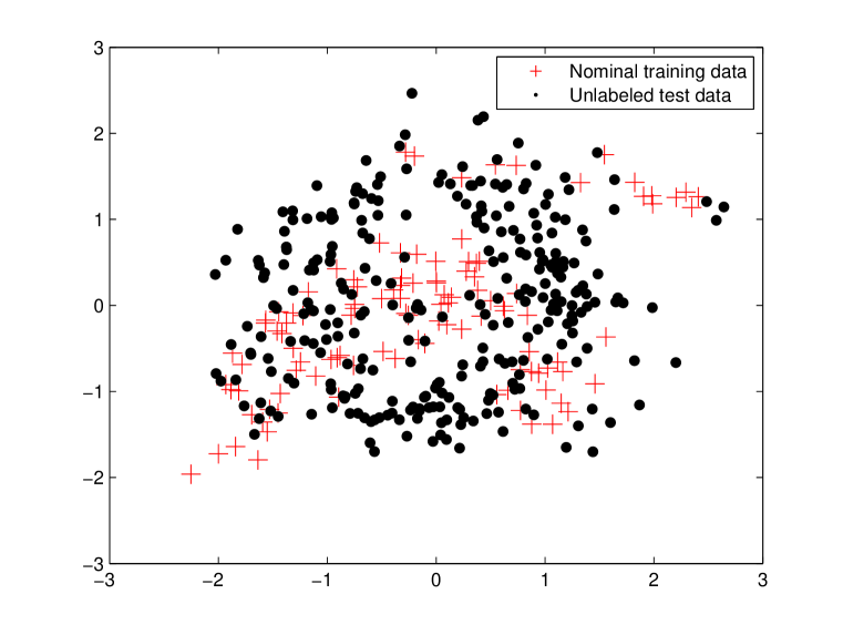
(a) Configuration of banana data

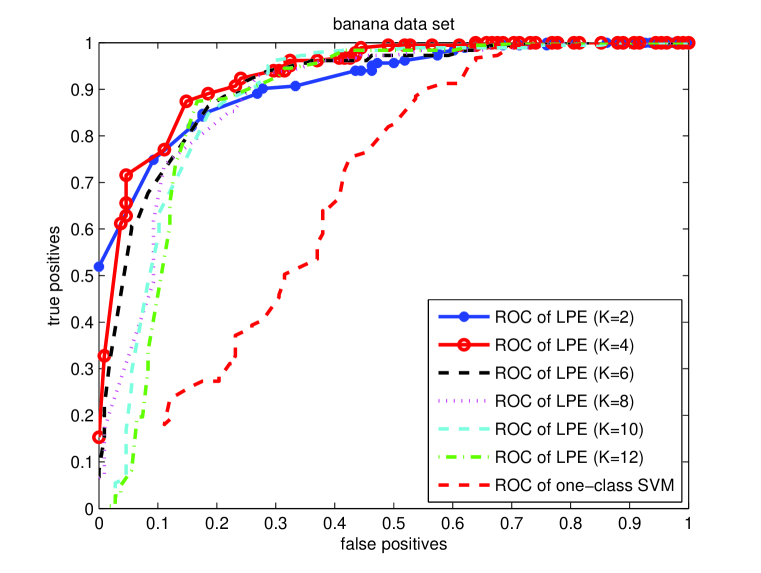
(b) SVM vs. K-LPE for Banana Data

Figure 2: Performance Robustness of LPE;(a) The configuration of the nominal training points (red ‘+’) and unlabeled test points (black ‘ $\bullet$’) for the banana dataset [19]; (b) Empirical ROC curve of $K$-LPE on the banana dataset with $K=2,4,6,8,10,12$ (with $n=400$) vs the empirical ROC curve of one class SVM developed in [9].

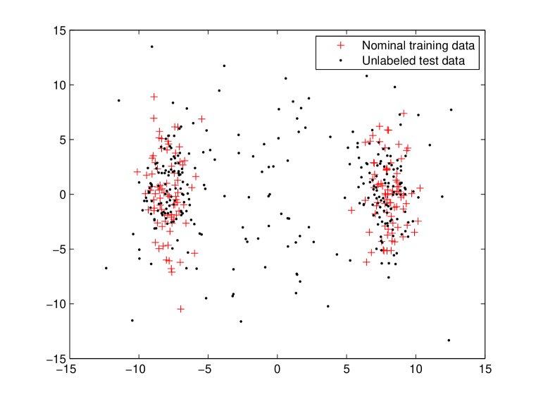
(a) Configuration of data

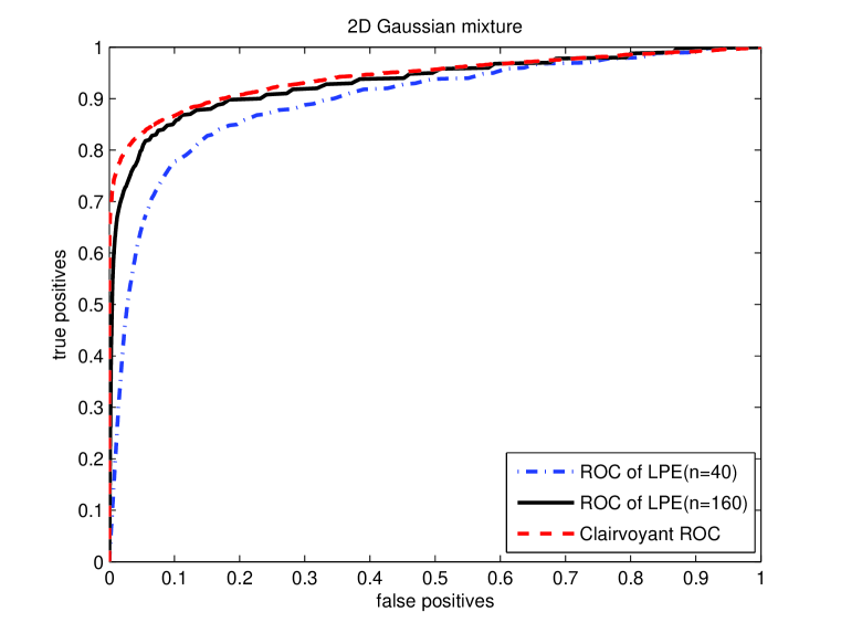
(b) Clairvoyant vs. K-LPE

Figure 3: Clairvoyant ROC curve vs. K-LPE; (a) Configuration of the nominal training points and unlabeled test points for the data given by Equation 10; (b) Averaged (over $15$ trials) empirical ROC curves of $K$-LPE algorithm vs clairvoyant ROC curve (when $f_{0}$ is given by Equation 10) for $K=6$ and for different values of $n$ ($n=40,160$).

In Figure 3, we apply our $K$-LPE to another 2D artificial example where the nominal distribution $f_{0}$ is a mixture Gaussian and the anomalous distribution is very close to uniform (see Figure 3(a) for their configuration):

$$f_{0}\sim\frac{1}{2}\mathcal{N}\left(\begin{bmatrix}8\\ 0\end{bmatrix},\begin{bmatrix}1&0\\ 0&9\end{bmatrix}\right)+\frac{1}{2}\mathcal{N}\left(\begin{bmatrix}-8\\ 0\end{bmatrix},\begin{bmatrix}1&0\\ 0&9\end{bmatrix}\right),\quad f_{1}\sim\mathcal{N}\left(0,\begin{bmatrix}49&0\\ 0&49\end{bmatrix}\right)$$ (10)

In this example, we can exactly compute the optimal ROC curve. We call this curve the Clairvoyant ROC (the red dashed curve in Figure 3(b)). The other two curves are averaged (over $15$ trials) empirical ROC curves with respect to different sizes of training sample ($n=40,160$) for $K=6$. Larger $n$ results in better ROC curve. We see that for a relatively small training set of size $160$ the average empirical ROC curve is very close to the clairvoyant ROC curve.

Next, we ran LPE on three real-world datasets: Wine, Ionosphere[20] and MNIST US Postal Service (USPS) database of handwritten digits. The procedure and setup of the experiments is almost the same as the that of the Banana data set. However, there are two differences. (1) If the number of different labels is greater than two, we always treat points with one particular label as nominal($+1$) and regard the points with other labels as anomalous($-1$). For example, for the USPS dataset, we regard instances of digit $0$ as nominal training samples and instances of digits $1,\cdots,9$ as anomaly. (2) For high dimensional data set, the data points are normalized to be within $[0,1]^{d}$ and we use geodesic distance [14](instead of Euclidean distance) as the input to LPE.

Figure 4: ROC curves on real datasets via LPE; (a) Wine dataset with $D=13,n=39,\epsilon=0.9$; (b) Ionosphere dataset with $D=34,n=175,K=9$; (c) USPS dataset with $D=256,n=400,K=9$.

The ROC curves of these three datasets are shown in Figure 4. In Wine dataset, the dimension of the feature space is $13$. The training set is composed of $39$ data points and we apply the $\epsilon$-LPE algorithm with $\epsilon=0.9$. The test set is a mixture of 20 nominal points and $158$ anomaly points (ground truth). In Ionosphere dataset, the dimension of the feature space is $34$. The training set is composed of $175$ data points and we apply the $K$-LPE algorithm with $K=9$. The test set is a mixture of $50$ nominal points and $126$ anomaly points (ground truth). In USPS dataset, the dimension of the feature space is $16\times 16=256$. The training set is composed of $400$ data points and we apply the $K$-LPE algorithm with $K=9$. The test set is a mixture of $367$ nominal points and $33$ anomaly points (ground truth).

For comparison purposes we note that for the USPS data set by setting $\alpha=0.5$ we get empirical false-positive $6.1\%$ and empirical false alarm rate $5.7\%$ (In contrast $FP=7\%$ and $FA=9\%$ with $\nu=5\%$ for OC-SVM as reported in [9]). Practically we find that $K$-LPE is more preferable to $\epsilon$-LPE due to easiness of choosing the parameter $K$. We find that the value of $K$ is relatively independent of dimension $d$. As a rule of thumb we found that setting $K$ around $n^{2/5}$ was generally effective.

5 Conclusion

In this paper, we proposed a novel non-parametric adaptive anomaly detection algorithm which leads to a computationally efficient solution with provable optimality guarantees. Our algorithm takes a K-nearest neighbor graph as an input and produces a score for each test point. Scores turn out to be empirical estimates of the volume of minimum volume level sets containing the test point. While minimum volume level sets provide an optimal characterization for anomaly detection, they are high dimensional quantities and generally difficult to reliably compute in high dimensional feature spaces. Nevertheless, a sufficient statistic for optimal tradeoff between false alarms and misses is the volume of the MV set itself, which is a real number. By computing score functions we avoid computing high dimensional quantities and still ensure optimal control of false alarms and misses. The computational cost of our algorithm scales linearly in dimension and quadratically in data size.

References

- [1] C. Campbell and K. P. Bennett, “A linear programming approach to novelty detection,” in Advances in Neural Information Processing Systems 13. MIT Press, 2001, pp. 395–401.
- [2] M. Markou and S. Singh, “Novelty detection: a review – part 1: statistical approaches,” Signal Processing, vol. 83, pp. 2481–2497, 2003.
- [3] R. Ramaswamy, R. Rastogi, and K. Shim, “Efficient algorithms for mining outliers from large data sets,” in Proceedings of the ACM SIGMOD Conference, 2000.
- [4] R. Vert and J. Vert, “Consistency and convergence rates of one-class svms and related algorithms,” Journal of Machine Learning Research, vol. 7, pp. 817–854, 2006.
- [5] D. Tax and K. R. Mller, “Feature extraction for one-class classification,” in Artificial neural networks and neural information processing, Istanbul, TURQUIE, 2003.
- [6] R. El-Yaniv and M. Nisenson, “Optimal singl-class classification strategies,” in Advances in Neural Information Processing Systems 19. MIT Press, 2007.
- [7] I. V. Nikiforov and M. Basseville, Detection of abrupt changes: theory and applications. Prentice-Hall, New Jersey, 1993.
- [8] K. Zhang, M. Hutter, and H. Jin, “A new local distance-based outlier detection approach for scattered real-world data,” March 2009, arXiv:0903.3257v1[cs.LG].
- [9] B. Schlkopf, J. C. Platt, J. Shawe-Taylor, A. J. Smola, and R. Williamson, “Estimating the support of a high-dimensional distribution,” Neural Computation, vol. 13, no. 7, pp. 1443–1471, 2001.
- [10] D. Tax, “One-class classification: Concept-learning in the absence of counter-examples,” Ph.D. dissertation, Delft University of Technology, June 2001.
- [11] G. R. G. Lanckriet, L. E. Ghaoui, and M. I. Jordan, “Robust novelty detection with single-class MPM,” in Neural Information Processing Systems Conference, vol. 18, 2005.
- [12] C. Scott and R. D. Nowak, “Learning minimum volume sets,” Journal of Machine Learning Research, vol. 7, pp. 665–704, 2006.
- [13] A. O. Hero, “Geometric entropy minimization(GEM) for anomaly detection and localization,” in Neural Information Processing Systems Conference, vol. 19, 2006.
- [14] J. B. Tenenbaum, V. de Silva, and J. C. Langford, “A global geometric framework fo nonlinear dimensionality reduction,” Science, vol. 290, pp. 2319–2323, 2000.
- [15] M. Bernstein, V. D. Silva, J. C. Langford, and J. B. Tenenbaum, “Graph approximations to geodesics on embedded manifolds,” 2000.
- [16] S. T. Roweis and L. K. Saul, “Nonlinear dimensionality reduction by local linear embedding,” Science, vol. 290, pp. 2323–2326, 2000.
- [17] C. McDiarmid, “On the method of bounded differences,” in Surveys in Combinatorics. Cambridge University Press, 1989, pp. 148–188.
- [18] L. Devroye, L. Györfi, and G. Lugosi, A Probabilistic Theory of Pattern Recognition. Springer Verlag New York, Inc., 1996.
- [19] “Benchmark repository.” [Online]. Available: http://ida.first.fhg.de/projects/bench/benchmarks.htm
- [20] A. Asuncion and D. J. Newman, “UCI machine learning repository,” 2007. [Online]. Available: http://www.ics.uci.edu/mlearn/MLRepository.html