Quantum Decoherence of Photons in the Presence of Hidden U(1)s

Abstract

Many extensions of the standard model predict the existence of hidden sectors that may contain unbroken abelian gauge groups. We argue that in the presence of quantum decoherence photons may convert into hidden photons on sufficiently long time scales and show that this effect is strongly constrained by CMB and supernova data. In particular, Planck-scale suppressed decoherence scales $D\propto\omega^{2}/M_{\rm Pl}$ (characteristic for non-critical string theories) are incompatible with the presence of even a single hidden U$(1)$. The corresponding bounds on the decoherence scale are four orders of magnitude stronger than analogous bounds derived from solar and reactor neutrino data and complement other bounds derived from atmospheric neutrino data.

I Motivation

Physics beyond the standard model typically predicts the existence of hidden sectors containing extra matter with new gauge interactions. There is no compelling reason why these extra sectors should be very massive if their interaction with standard model matter is sufficiently weak. This can be accomplished, e.g., in extra dimensional extensions with a geometric separation of sectors or in models where tree-level interactions are absent and higher order corrections suppressed by the scale of messenger masses.

The presence of these light hidden sectors can have various observable effects. For example, in the case of kinetic mixing Holdom:1985ag ; Dienes:1996zr between a hidden U$(1)$ and the electromagnetic U$(1)$, hidden sector matter can receive small fractional electro-magnetic charges. These mini-charged particles can have a strong influence on early Universe physics and astrophysical environments Raffelt:1996wa . If the hidden sector U$(1)$ is slightly broken by a Higgs or Stückelberg mechanism we can have a situation analogous to neutrino systems with characteristic oscillation patterns between photons and hidden photons over sufficiently long baselines Okun:1982xi .

Here we concentrate on another effect induced by the presence of these light hidden sectors: the sensitivity of photon propagation to sources of quantum decoherence, e.g. quantum gravity effects Hawking:1982dj . A heuristic picture describes space-time at the Planck scale as a foamy structure Wheeler:1957mu , where virtual black holes pop in and out of existence on a time scale allowed by Heisenberg’s uncertainty principle Hawking:1995ag . This can lead to a loss of quantum information across their event horizons, providing an “environment” that might induce quantum decoherence of apparently isolated matter systems Hawking:1982dj .

It is an open matter of debate whether quantum decoherence induced by a quantum theory of gravity would simultaneously preserve Poincare invariance and locality Hawking:1982dj ; Hawking:1995ag ; Ellis:1983jz ; Banks:1983by ; Unruh:1995gn . A violation of energy and momentum conservation by particle reactions with a space-time foam could be reflected by an (energy dependent) effective refractive index in vacuo AmelinoCamelia:1996pj . This could be tested, e.g., by the measurement of the arrival time of gamma rays or high energy neutrinos at different energies or by the propagation of ultra-high energy cosmic rays GonzalezMestres:1997dr .

If, on the other hand, Poincare invariance is preserved, the presence of a non-trivial space-time vacuum can still be signaled by decoherence effects in systems of stable elementary particles Ellis:1983jz . A particularly interesting and well-studied case are neutrino systems, where the interplay between mixing, mass oscillation and decoherence can influence atmospheric, solar and reactor neutrino data Lisi:2000zt ; Gago:2002na ; Fogli:2007tx , as well as flavour composition of astrophysical high-energy neutrino fluxes Hooper:2004xr ; Anchordoqui:2005gj .

If hidden sectors contain unbroken abelian gauge groups it is also feasible that the system of the electromagnetic photon ($\gamma_{0}$) and hidden photons ($\{\gamma_{i}\}$ with $i\geq 1$) experience energy and momentum conserving decoherence effects: transitions between different photon “species”, $\gamma_{\mu}\to\gamma_{\nu}$, are allowed by gauge and Poincare invariance. This is the only alternative system to neutrinos involving a stable and neutral elementary particle of the standard model, which can experience these decoherence effects on extremely long (cosmological) time scales.

The outline of this paper is as follows. We will start in Sect. II with an outline of the Lindblad formalism of quantum decoherence. We will then discuss in Sect. III the effect of photon decoherence on the Planck spectrum of the cosmic microwave background and the luminosity distance of type Ia supernovae, respectively. This enables us to derive strong limits on various decoherence models. We comment in Sect. IV on the interplay of decoherence and photon interactions and outline a possible mechanism to extend the survival probability of extra-galactic TeV gamma rays. We finally summarize in Sect. V.

II Quantum Decoherence

The Lindblad formalism is a general approach to quantum decoherence that does not require any detailed knowledge of the environment Lindblad:1975ef . In the presence of decoherence the modified Liouville equation can be written in the form

$$\frac{\partial\rho}{\partial t}=-{\rm i}[H,\rho]+\mathcal{D}[\rho]\,.$$ (1)

The Hamiltonian $H$ can include possible background contributions, e.g. plasma effects for the photon. However, this does not effect the evolution of the density matrix in the absence of mixing between the gauge bosons. The decoherence term $\mathcal{D}$ in the modified Liouville equation (1) can be written as

$${\cal D}[\rho]=\frac{1}{2}\sum_{j}\left([b_{j},\,\rho\,b_{j}^{\dagger}]+[b_{j}\,\rho,\,b_{j}^{\dagger}]\right)\,,$$ (2)

where $\{b_{j}\}$ is a sequence of bounded operators acting on the Hilbert space of the open quantum system, ${\cal H}$, and satisfying $\sum_{j}b^{\dagger}_{j}b_{j}\in{\cal B}({\cal H}),$ where ${\cal B}({\cal H})$ indicates the space of bounded operators acting on ${\cal H}$. The dynamical effects of spacetime on a microscopic system can then be interpreted as the existence of an arrow of time which in turn makes possible the connection with thermodynamics via an entropy. The monotonic increase of the von Neumann entropy, $S(\rho)=-{\rm Tr}(\rho\ln\rho)$, implies the hermiticity of the Lindblad operators, $b_{j}=b_{j}^{\dagger}$ Benatti:1987dz . In addition, the conservation of energy and momentum can be enforced by taking $[P_{\mu},b_{j}]=0$.

We will assume in the following that there is a total of $N$ abelian gauge bosons $\gamma_{\mu}$ with $\mu=0,\ldots,N-1$ including the photon $\gamma_{0}$. The solution to Eq. (1) is outlined in Appendix A. For simplicity, we assume degeneracy of the decoherence parameters $D_{i}=D$ which simplifies the photon survival probability after a distance $x=t=L$ significantly (see App. A),

$$P_{\gamma\to\gamma}=\frac{1}{N}+\frac{N-1}{N}e^{-DL}\,.$$ (3)

The energy behavior of $D$ depends on the dimensionality of the operators $b_{j}.$ We can estimate the energy dependence from gauge invariance. Possible combinations of the field strength tensors $F_{\mu\nu}$ and $G_{\mu\nu}$ of the two U$(1)$s are Hawking:1982dj $b_{j}\propto(F_{\mu\nu}G^{\mu\nu})^{j}\propto\omega^{j}$. This restriction of the energy behavior to non-negative powers of $\omega$ may possibly be relaxed when the dissipative term is directly calculated in the most general space-time foam background Anchordoqui:2005gj .

An interesting example is the case where the dissipative term is dominated by the dimension-4 operator $b_{1}$ yielding the energy dependence $D\propto\omega^{2}/M_{\rm Pl}.$ This is characteristic of non-critical string theories where the space-time defects of the quantum gravitational “environment” are taken as recoiling $D$-branes, which generate a cellular structure in the space-time manifold Ellis:1996bz .

III Observational Constraints

In the following we will investigate the limits on quantum decoherence in the presence of hidden massless U$(1)$s from cosmological and astrophysical observations. Unless otherwise stated, we will make the conservative assumption that there exists only a single hidden U$(1)$ in addition to the standard model ($N=2$) and that the decoherence rate of photons can be parametrized as

$$D(z,\omega)=(1+z)^{p+1}D_{*}\frac{\omega^{p+1}}{M^{p}_{\rm QD}}\,,$$ (4)

where $M_{\rm QD}$ is the scale of quantum decoherence, not necessarily the Planck scale. We will consider the scale dependencies $p=0,\pm 1,\pm 2$.

The differential flux of photons from a source at redshift $z$ is reduced by the exponential factor

$$P_{\gamma\to\gamma}(z,\omega)=\frac{1}{2}+\frac{1}{2}\exp\left[-\int_{0}^{z}{\rm d}\ell^{\prime}\,D(z^{\prime},\omega)\right]\,,$$ (5)

where the propagation distance $\ell$ is given by ${\rm d}z=H(z)(1+z){\rm d}\ell$ with Hubble parameter $H$. The Hubble parameter at redshift $z$ is given by $H^{2}(z)=H_{0}^{2}[(1-\Omega_{m}-\Omega_{r})+\Omega_{m}(1+z)^{3}+\Omega_{r}(1+z)^{4}]$ where $\Omega_{m}h^{2}\simeq 0.128$ and $\Omega_{r}h^{2}\simeq 2.47\times 10^{-5}$. The present Hubble expansion is $H_{0}=h\,100\,{\rm km}\,{\rm s}^{-1}\,{\rm Mpc}^{-1}$ with $h\simeq 0.73$ Amsler:2008zzb .

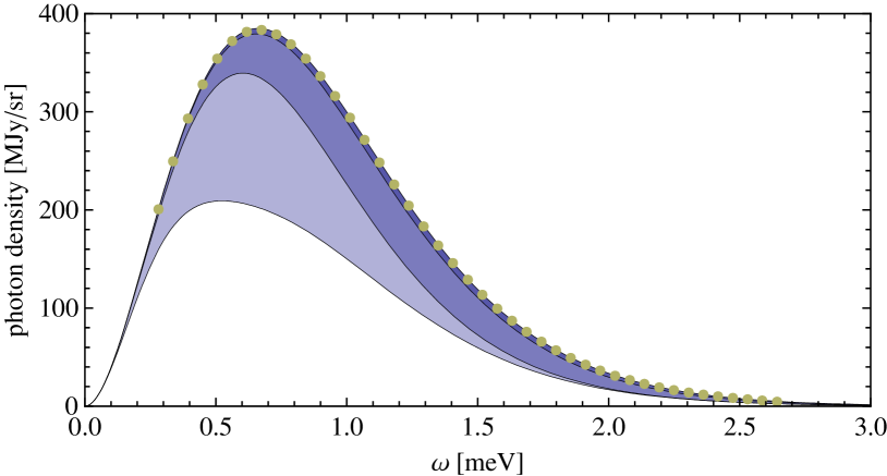
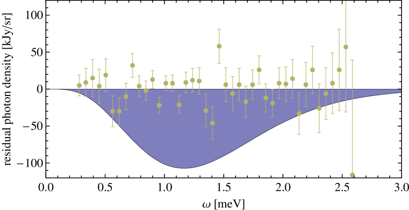
Figure 1: Modification of the CMB spectrum by decoherence effects. The dots show the residual CMB spectrum measured by COBE/FIRAS FIRAS ($1$Jy (Janksy) $\equiv 10^{-26}$ W m^-1 Hz^-1). The upper panel shows the effect of $D_{*}=0.01,0.1,1$ and the lower panel $D_{*}=10^{-4}$. The curves show the accumulated deficit in photons compared to the “no decoherence” case. (A different shadowing is included to guide the eye.)

Model	CMB	SNe	reactor&solar $\nu$	atmospheric $\nu$
$p=-2$	$9.5\times 10^{-97}$	$3.9\times 10^{-90}$	$8.3\times 10^{-65}$	$1.0\times 10^{-59}$
$p=-1$	$9.7\times 10^{-66}$	$3.4\times 10^{-62}$	$8.8\times 10^{-44}$	-
$p=0$	$3.9\times 10^{-35}$	$2.9\times 10^{-34}$	$1.0\times 10^{-22}$	$1.2\times 10^{-27}$
$p=1$	$1.3\times 10^{-5}$	$2.3\times 10^{-6}$	$0.11$	$1.6\times 10^{-12}$
$p=2$	$3.5\times 10^{23}$	$1.8\times 10^{22}$	-	$910$

Table 1: The $3\sigma$ limits on $D_{*}$ derived from the COBE/FIRAS data FIRAS and SN data Kowalski:2008ez for a decoherence scale given by Eq. (4). We assume $N=2$ and $M_{\rm QD}=M_{\rm Pl}$. Note that the limits are in general stronger for $N>2$ by up to a factor $2$. For comparison the last two columns show the limits from reactor and solar  Fogli:2007tx , and atmospheric neutrinos  Lisi:2000zt ; Collaboration:2009nf .

III.1 CMB Distortions

In the standard big bang cosmology the cosmic microwave background (CMB) forms at a redshift of about $z_{\rm CMB}\simeq 1100$ after recombination of electrons and (mostly) protons in the expanding and cooling Universe. The CMB is well described by a Planck spectrum with a temperature of $T=2.725\pm 0.001$ K FIRAS ,

$$\frac{{\rm d}^{2}n}{{\rm d}\omega{\rm d}\Omega}=\frac{1}{2\pi^{2}}\frac{\omega^{3}}{\exp\left(\frac{\omega}{T}\right)-1}\,.$$ (6)

The high degree of accuracy (better than $1$ in $10^{4}$ around $1$ meV) between the CMB measurement and cosmological predictions is an ideal probe for exotic physics that could have effected the CMB photons in the redshift range $0<z<z_{\rm CMB}$ with energies from meV ($z=0$) to eV ($z=z_{\rm CMB}$).

The influence of light particles coupling to the CMB has been studied previously for the case of axion-like particles Mirizzi:2005ng , mini-charged particles Melchiorri:2007sq and massive hidden photons with kinetic mixing Jaeckel:2008fi . In the case of photon absorption or decoherence the observed spectrum is modified as

$$\frac{{\rm d}^{2}n^{\rm obs}}{{\rm d}\omega{\rm d}\Omega}=P_{\gamma\to\gamma}(z_{\rm CMB},\omega)\,\frac{{\rm d}^{2}n}{{\rm d}\omega{\rm d}\Omega}\,.$$ (7)

As an illustration of the effect of decoherence, Fig. 1 shows the distortion of the CMB spectrum for the case $p=1$ and $M_{\rm QD}=M_{\rm Pl}\simeq 1.2\times 10^{19}$ GeV for $D_{*}=0.01,0.1,1$ (upper panel) and $D_{*}=10^{-4}$ (lower panel). The $3\sigma$ limits from a $\chi^{2}$-fit of various models to the COBE/FIRAS data FIRAS are shown in Tab. 1 (see also upper left panel in Fig. 3). For comparison, the two right columns show limits on the decoherence parameter derived from solar and reactor neutrino data Fogli:2007tx and atmospheric neutrino data Lisi:2000zt ; Collaboration:2009nf . We will comment on how to compare these bounds at the end of the section.

III.2 SN Dimming

Also the luminosity distance measurements of cosmological standard candles like type Ia supernovae (SNe) Riess:1998cb ; Kowalski:2008ez are able to test feeble photon absorption and decoherence effects. The luminosity distance $d_{L}$ is defined as

$$d_{L}(z)\equiv\sqrt{\frac{\mathcal{L}}{4\pi F}}\,,$$ (8)

where $\mathcal{L}$ is the luminosity of the standard candle (assumed to be sufficiently well-known) and $F$ the measured flux. In a homogeneous and isotropic universe this is predicted to be

$$d_{L}(z)=(1+z)\,a_{0}\,\Phi\left(\int_{0}^{z}\frac{{\rm d}z^{\prime}}{a_{0}H(z^{\prime})}\right)\,,$$ (9)

with $a_{0}^{-1}=H_{0}\sqrt{|1-\Omega_{\rm tot}|}$ and $\Phi_{k}(\xi)=(\sinh\xi,\xi,\sin\xi)$ for spatial curvature $k=-1,0,1$, respectively. If the photon flux of a source, located at distance $z$ and observed in a (small) frequency band centered at $\omega_{\star}$, is attenuated by photon interactions or quantum decoherence the observed luminosity distance increases as

$$d_{L}^{\,\rm obs}(z)=\frac{d_{L}(z)}{\sqrt{P_{\gamma\to\gamma}(z,\omega_{\star})}}\,.$$ (10)

The apparent extension of the luminosity distance by photon interactions and oscillations has been investigated in the context of axion-like particles Csaki:2001yk ; Mirizzi:2005ng , hidden photons Evslin:2005hi , chameleons Burrage:2007ew and mini-charged particles Ahlers:2009kh . One of the main attractions of these models is the possibility that the conclusions about the energy content of our Universe drawn from the Hubble diagram can be dramatically altered. We will briefly comment on this possibility at the end of this section.

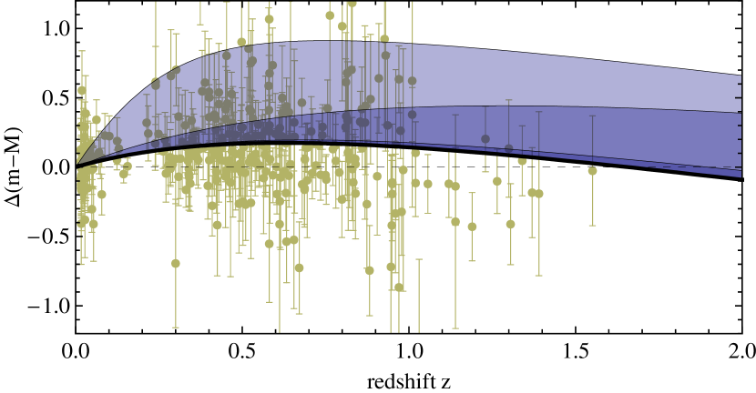
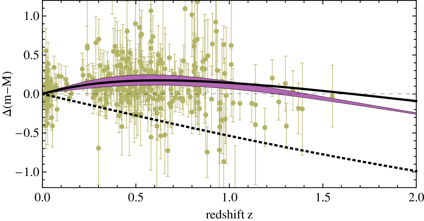
Figure 2: Upper Panel: Enhanced SNe dimming by decoherence effects assuming $N=2$, $p=1$, $M_{\rm QD}=M_{\rm Pl}$ and $D_{*}=10^{-6},10^{-5},10^{-4}$ assuming sources observed in a frequency interval centered at $\omega_{\star}=1$ eV. The dots show the SNe Ia “union” compilation from Ref. Kowalski:2008ez . The luminosity distance $d_{L}$ is shown by the difference $\Delta(m-M)$ to an empty ($\Omega_{\rm tot}=0$) flat universe. The thin lines show the accumulated deficit in photons compared to the “no decoherence” case (standard $\Lambda$CDM model) indicated by the thick line. Lower Panel: As the upper panel, but now showing also a flat CDM model with $\Omega_{m}=1$ and $\Omega_{\Lambda}=0$ (dotted line). For illustration, we consider a hidden photon model with $p=1$, $N=2$ and $D_{*}=6\times 10^{-6}$ and show the dimming for the B ($\lambda_{\star}\simeq 440$ nm, upper line) and V ($\lambda_{\star}\simeq 550$ nm, lower line) band. Whereas the overall dimming effect is practically indistinguishable from the $\Lambda$CDM model, the strong reddening of the starlight from the energy dependence of $D\propto\omega^{2}/M_{\rm Pl}$ is challenged by the data KowalskiPC .

As an example, the upper panel of Fig. 2 shows the effect on quantum decoherence in the $\Lambda$CDM model assuming a single hidden U$(1)$ ($N=2$). The luminosity distance of the SNe is shown as the difference between their measured apparent magnitude $m$ and their known absolute magnitude $M$,

$$m-M=5\log_{10}d_{L,{\rm Mpc}}+25\,.$$ (11)

As in the previous case we can derive $3\sigma$ limits for various decoherence models that are shown in Tab. 1 (see also upper right panel in Fig. 3). The limits on Planck-scale suppressed decoherence ($p=1,2$) from SN dimming are slightly stronger than the CMB limits.

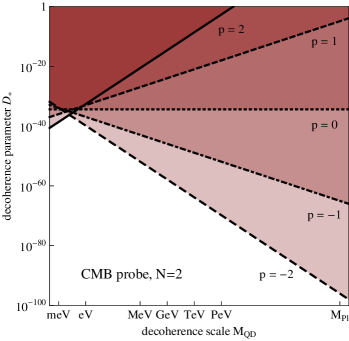
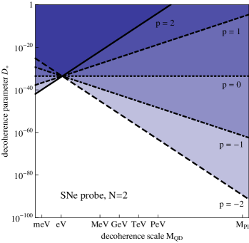
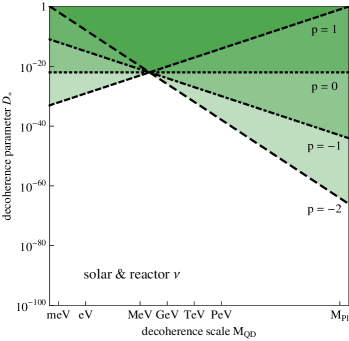
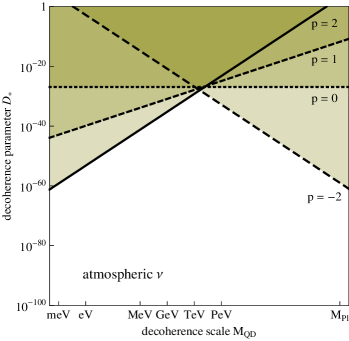
Figure 3: 3$\sigma$ C.L. upper bound on $D_{*}$ as a function of $M_{\rm QD}$ for various models of $D$. We show the bounds on from the CMB FIRAS (upper left panel) and from type Ia SNe Kowalski:2008ez (upper right panel) for various models $p=0,\pm 1,\pm 2$ of the decoherence parameter $D=D_{*}\omega^{p+1}/M_{\rm QD}^{p}$. Darker colors indicate regions which are excluded by multiple models. Note that the limits become generally stronger for $N>2$ by up to a factor $2$. For comparison, the lower plots show the limits from solar and reactor neutrino data Fogli:2007tx ($3\sigma$ C.L.) and atmospheric neutrino data, Lisi:2000zt ($3\sigma$ C.L.) and Collaboration:2009nf ($90$% C.L.).

However, we would like to emphasize that these limits depend on the cosmological model and the normalization of the SN data. If the SN dimming by photon decoherence is strong this can have an effect on the evaluation of cosmological data. We give an example in the lower panel of Fig. 2 where the decoherence effect could even be able to reproduce the observed SN luminosities from a CDM model. Note, that this model is not excluded by the corresponding CMB limits, though it is not compatible with the analogous bound from atmospheric neutrinos. In addition, one has to keep in mind that the photon frequency dependence of the parameter $D$ causes a color excess (unless $p=-1$) which is in conflict with observation Kowalski:2008ez . For the example shown in the right panel of Fig. 2 the color excess between the B and V band of the form, $E[{\rm B-V}]\equiv\Delta(m-M)_{\rm B}-\Delta(m-M)_{\rm V}$, is larger than $0.8$ for redshifts $0.2\lesssim z\lesssim 0.8$, more than twice the median color excess observed from SNe at this distance KowalskiPC . Moreover, photon absorption as a SN dimming mechanism would violate the cosmic distance-duality, i.e. the luminosity and angular diameter distance relation $d_{L}/d_{A}=(1+z)^{2}$ Bassett:2003vu . Hence, it is unlikely that decoherence can fully account for SN dimming. Nevertheless, it could have an effect on the evaluation of cosmological data.

The dependence on $M_{\rm QD}$ of the upper bound on $D_{*}$ for various models of $D$ as derived from CMB distortions and SN dimming are summarized in the top panels of Fig. 3. The lower panels show analogous limits derived from solar and reactor neutrino data Fogli:2007tx as well as atmospheric neutrino results Lisi:2000zt ; Collaboration:2009nf . It is apparent from the plots (as the intersection of the bounds ) that these probes are based on different energy scales, meV-eV in the case of the CMB, eV in the case of SNe, multi-MeV in the case of solar and reactor neutrino data and multi-TeV in the case of atmospheric neutrinos. Consequently we see that for models with $p\leq 0$ the bounds from from CMB distortions and SN dimming are the strongest. One must however bear in mind that while bounds from neutrino data are “unavoidable” once the quantum decoherence effects exist, the effects on photon propagation discussed here rely on the extra assumption of the presence of massless hidden $U(1)$’s. Besides this, we also note that, generically decoherence effects that grow with energy are better constrained from higher energy atmospheric neutrino data. For example for the case $D\propto\omega^{2}/M_{\rm QD}$ ($p=1$ in our notation) the possible decoherence of photons in the presence of a single hidden U$(1)$ is about four (five) orders of magnitude stronger constrained from CMB (SNe) data than the corresponding limit from solar and reactor neutrino data Fogli:2007tx (cf. Tab. 1) but the bound derived from atmospheric neutrinos Collaboration:2009nf is much stronger.

The dimensionless parameter $D_{*}$ appearing in our definition of the decoherence scale (4) is naturally expected to be of order $1$. Hence, atmospheric neutrino data already severely constraints Planck-scale suppressed decoherence of the form $D=D_{*}\omega^{2}/M_{\rm Pl}$. Similarly, our analogous limits on photon decoherence in the presence of hidden U$(1)$s require $D_{*}\ll 1$ for $p=1$. In reverse, a quantum theory of gravity predicting Planck-scale suppressed decoherence is not compatible with the existence of unbroken hidden U$(1)$s unless, unnaturally, $D_{*}\ll 1$.

Higher order quantum decoherence with $p\geq 2$ is so far only weakly constrained by neutrino systems or by photon/hidden photon systems in the meV to eV energy range. We will speculate in the following section, how high energy gamma ray sources could possibly explore this unconstrained parameter space.

IV Photon Propagation

Decoherence effects can also have interesting effects on the propagation of photons in the presence of photon absorption. We can account for photon absorption effects in the Liouville equation (1) by a contribution

$$\mathcal{D}_{\Gamma}[\rho]=-\frac{\Gamma}{2}\{\Pi_{0},\rho\}\,,$$ (12)

where $\Gamma=1/\lambda$ is the photon absorption rate, e.g. in the intergalactic photon background (BG) via $\gamma+\gamma_{\rm BG}\to e^{+}+e^{-}$, and $\Pi_{0}$ is the photon projection operator.

The photon survival probability in the presence of a single hidden U$(1)$ can be readily solved from the modified Liouville equation and gives (see App. A for details)

$$P_{\gamma\to\gamma}=e^{-\frac{L}{2}(D+\Gamma)}\bigg{[}\cosh\left(\frac{L}{2}\sqrt{D^{2}+\Gamma^{2}}\right)\\ -\frac{\Gamma}{\sqrt{D^{2}+\Gamma^{2}}}\sinh\left(\frac{L}{2}\sqrt{D^{2}+\Gamma^{2}}\right)\bigg{]}\,.$$ (13)

We can estimate the sensitivity of extra-galactic TeV gamma ray sources to decoherence effects as

$$D_{*}\sim 10^{-38+16p}\left(\frac{M_{\rm QD}}{M_{\rm Pl}}\right)^{p}\left(\frac{\rm TeV}{\omega}\right)^{p+1}\left(\frac{\rm kpc}{L}\right)\,.$$ (14)

In particular for $M_{\rm QD}\sim M_{\rm Pl}$ , $D_{*}\sim 10^{-22}$ for $p=1$ or $D_{*}\sim 10^{-6}$ for $p=2$. Hence, this probe has the potential to be more sensitive to Planck-scale suppressed decoherence than existing neutrino data Lisi:2000zt ; Collaboration:2009nf by many orders of magnitude. We will discuss in the following possible signals of decoherence in the spectra of TeV gamma ray sources.

Figure 4 shows the survival probability for three different values of $D$. The functional behaviour can be easily understood as follows: The hidden U$(1)$ serves as an invisible “storage” of photons during propagation. If $D\lambda\gg 1$ decoherence quickly equalizes the number of photons and hidden photons. This results into a decrease of the photon survival probability to $1/2$ (for $N=2$) for $L\lesssim\lambda$. On the other hand, inelastic scattering only affects photons. Therefore at larger $L$ photons can be “replenished” by the decoherence of the unabsorbed hidden photons into photons. Hence, for propagation distances $L>\lambda$ the presence of hidden photons increases the photon survival probability.

For the general case of $N$ U$(1)$s and strong decoherence $D\gg\Gamma$ we can express the photon survival probability at a distance much larger than the decoherence scale $L\gg 1/D$ as (see App. A for details)

$$P_{\gamma\to\gamma}\simeq\frac{1}{N}\exp\left(-\frac{L}{N\lambda}\right)\,.$$ (15)

This can have an important effect on the spectra of TeV gamma ray sources. Firstly, if the onset of decoherence appears at energies covered by the spectra one could observe a step-like drop of the flux by a factor $1/N$. And secondly, as long as the absolute source emissivity of photons is unknown (such that the pre-factor $1/N$ in Eq. (15) gets renormalized), the expected spectral cut-offs of the sources could be shifted according to an extend photon interaction length $\lambda_{\rm eff}=N\lambda$. These effects can be clearly seen in Fig. 4 for the case $N=2$. For a TeV gamma ray source at $100$ Mpc and Planck-scale suppressed decoherence this requires $D_{*}\gg 10^{-27}$ ($D_{*}\gg 10^{-11}$) for $p=1$ ($p=2$). In comparing this with Tab. 1 and Fig. 3 we see that there is ample room for models that could have such an effect on the spectra.

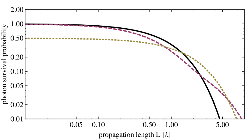
Figure 4: Photon survival probability in the presence of decoherence with a single hidden U$(1)$ ($N=2$). The black line shows the photon attenuation, e.g. in the inter-galactic photon background via $\gamma+\gamma_{\rm BG}\to e^{+}+e^{-}$, in the absence of decoherence ($D=0$). The dashed curve shows decoherence with $D\lambda=1$ and the dotted curve $D\lambda\gg 1$.

V Conclusions

We have discussed the effects of quantum decoherence of photons in the presence of hidden sector U$(1)$s. Quantum decoherence in the system of photon and hidden photons could be induced by a foam-like structure of space-time in a quantum theory of gravity, where virtual black holes pop in and out of existence at scales allowed by Heisenberg’s uncertainty principle.

We have shown that these decoherence effects are strongly constrained by the absence of photon disappearance in the cosmic microwave background. Furthermore quantum decoherence as an additional source of starlight dimming can also be constrained by the luminosity distance measurements of type Ia supernovae. Consequently based on the standard $\Lambda$CDM model we can derive constraints on the decoherence in the presence of hidden U$(1)$s. In principle, the decoherence effect could be strong enough to influence the evaluation of cosmological data. However, color dependencies in the dimming via photon decoherence are not favored by the data and could be used to derive further constraints.

Our main results are summarized in the upper panel of Fig. 3 and compared with the present bounds from non observation of decoherence effects in neutrino systems. For models with decoherence parameter $D$ constant or decreasing with energy, the bounds from from CMB distortions and SN dimming are the strongest. One must however bear in mind that while bounds from neutrino data are “unavoidable” once the quantum decoherence effects exist, the effects on photon propagation discussed here rely on the extra assumption of the presence of massless hidden U$(1)$s. We also note that, generically decoherence effects which grow with energy are better constrained from the higher energy atmospheric neutrino data.

We have also discussed the interplay between photon absorption and decoherence. This effect can become important for distant TeV gamma ray point-sources if the decoherence length is much smaller than the photon interaction length. Assuming $N-1$ additional U$(1)$s this could leave characteristic features in gamma ray spectra in the form of step-like drops by factors $1/N$ or by an effective increase of the absorption length $\lambda$ to $\lambda_{\rm eff}=N\lambda$.

Appendix A Lindblad Formalism

We outline the solution to the Liouville Eq. (1) in the presence of quantum decoherence. The density matrix $\rho$ and Lindblad operators $b_{j}$ can be expanded in a basis of hermitian matrices $F_{\mu}$ that satisfy the orthonormality condition ${\rm Tr}(F^{\dagger}_{\mu}F_{\nu})=\delta_{\mu\nu}/2$. Without loss of generality we consider a basis with $(F_{0})_{ij}=\delta_{ij}/\sqrt{2N}$. Explicitly, we have

$$\rho=\sum_{\mu}\rho_{\mu}F_{\mu}\,,\qquad b_{j}=\sum_{\mu}b^{(j)}_{\mu}F_{\mu}\,.$$ (16)

The free propagation of photons and hidden photons ($H=-{\rm i}\partial/\partial x$) can be readily solved in terms of “light-cone” coordinates $\hat{x}=(x-t)/2$ and $\hat{t}=(x+t)/2$. In these new coordinates Eq. (1) can be written $\partial\rho/\partial\hat{t}=\mathcal{D}[\rho]$.

Hence, the coefficients of the free equations of motion satisfy the differential equation

$$\frac{\partial}{\partial t}\rho_{\mu}=-\sum_{\nu}D_{\mu\nu}\rho_{\nu}\,,$$ (17)

with $D_{\mu 0}=D_{0\mu}=0$ and

$$D_{ij}=\frac{1}{2}\sum_{k,l,m,n}b^{(n)}_{m}f_{iml}b^{(n)}_{k}f_{jkl}\,,$$ (18)

where $f_{ijk}$ are structure constants defined by $[F_{i},F_{j}]=i\sum_{k}f_{ijk}F_{k}$.

The solution of $\partial_{t}\rho_{0}=0$ is trivial and requires $\rho_{0}(t)=\rho_{0}=2{\rm Tr}(\Pi_{\alpha}F_{0})=\sqrt{2/N}$ for all species $\alpha$. If $D_{ij}$ is diagonalizable by a matrix $M$, $(M^{-1}DM)_{ij}=D_{i}\delta_{ij}$, we can write the final solution as

$$P_{\gamma\to\gamma}=\frac{1}{N}+\frac{1}{2}\sum_{i,k,j}e^{-D_{k}t}\rho_{i}(0)M_{ik}M^{-1}_{kj}\rho_{j}(0)\,.$$ (19)

This reduces to Eq. (3) in the case $D_{i}=D$ using $2=\sum_{\mu}\rho_{\mu}^{2}$ following from $\rho^{2}(0)=\rho(0)$ and ${\rm Tr}[\rho]=1$.

We can extend the Lioville Eq. (1) by a photon decay term of the form (12). The modified equation can be readily solved in the case of $N=2$, taking $F_{i}=\frac{1}{2}\sigma_{i}$ with Pauli matrices $\sigma_{i}$. In this basis the photon projection operator in the term (12) has the form $\Pi_{0}=F_{0}+F_{3}$. And the general solution of the photon survival probability is given in Eq. (13).

In the case of strong decoherence, i.e. at propagation distances $L\gg 1/D$ and $D\gg\Gamma$, we can derive the asymptotic solution (15) of the general survival probability with $N$ U$(1)$s in the following way. In the presence of strong decoherence we can assume that at any step during the evolution ${\rm Tr}[\Pi_{\mu}\rho]\simeq{\rm Tr}[\Pi_{\nu}\rho]$ and, in particular, ${\rm Tr}[\rho]\simeq N{\rm Tr}[\Pi_{0}\rho]$. Since the trace of the decoherence term vanishes we can derive the asymptotic differential equation

$${\rm Tr}[\dot{\rho}]\simeq N{\rm Tr}[\Pi_{0}\dot{\rho}]\simeq-\Gamma{\rm Tr}[\Pi_{0}\rho]\,.$$ (20)

This has the solution (15), noting that $P_{\gamma\to\gamma}={\rm Tr}[\Pi_{0}\rho]$ and initially ${\rm Tr}[\Pi_{0}\rho(0)]=1/N$.

References

- (1)
- (2) B. Holdom, Phys. Lett. B 166, 196 (1986).
- (3) For estimations of the kinetic mixing scale in string or field theoretic setups see e.g. K. R. Dienes, C. F. Kolda and J. March-Russell, Nucl. Phys. B 492 (1997) 104 [arXiv:hep-ph/9610479]; S. A. Abel, M. D. Goodsell, J. Jaeckel, V. V. Khoze and A. Ringwald, JHEP 0807, 124 (2008) [arXiv:0803.1449 [hep-ph]]; M. Goodsell et al., [arXiv:0909.0515 [hep-ph]].
- (4) G. G. Raffelt, “Stars As Laboratories For Fundamental Physics,” Chicago, USA: Univ. Pr. (1996) 664 p; S. Davidson, S. Hannestad and G. Raffelt, JHEP 0005, 003 (2000) [arXiv:hep-ph/0001179].
- (5) L. B. Okun, Sov. Phys. JETP 56 (1982) 502 [Zh. Eksp. Teor. Fiz. 83 (1982) 892]; M. Ahlers et al., Phys. Rev. D 76 (2007) 115005 [arXiv:0706.2836 [hep-ph]].
- (6) S. W. Hawking, Commun. Math. Phys. 87, 395 (1982).
- (7) J. A. Wheeler, Annals Phys. 2, 604 (1957).
- (8) S. W. Hawking, Phys. Rev. D 53, 3099 (1996) [arXiv:hep-th/9510029].
- (9) J. R. Ellis, J. S. Hagelin, D. V. Nanopoulos and M. Srednicki, Nucl. Phys. B 241, 381 (1984).
- (10) W. G. Unruh and R. M. Wald, Phys. Rev. D 52, 2176 (1995) [arXiv:hep-th/9503024].
- (11) T. Banks, L. Susskind and M. E. Peskin, Nucl. Phys. B 244, 125 (1984).
- (12) G. Amelino-Camelia, J. R. Ellis, N. E. Mavromatos and D. V. Nanopoulos, Int. J. Mod. Phys. A 12, 607 (1997) [arXiv:hep-th/9605211]; G. Amelino-Camelia, J. R. Ellis, N. E. Mavromatos, D. V. Nanopoulos and S. Sarkar, Nature 393, 76 (1998) [arXiv:astro-ph/9712103].
- (13) See e.g., L. Gonzalez-Mestres, Proceedings of ICRC 1997, Durban, South Africa, [arXiv:physics/9705031]; S. R. Coleman and S. L. Glashow, Phys. Rev. D 59, 116008 (1999) [arXiv:hep-ph/9812418]; R. Aloisio, P. Blasi, P. L. Ghia and A. F. Grillo, Phys. Rev. D 62, 053010 (2000) [arXiv:astro-ph/0001258]; G. Amelino-Camelia and T. Piran, Phys. Rev. D 64, 036005 (2001) [arXiv:astro-ph/0008107]; J. R. Ellis, N. E. Mavromatos and D. V. Nanopoulos, Phys. Rev. D 63, 124025 (2001) [arXiv:hep-th/0012216]; F. W. Stecker and S. L. Glashow, Astropart. Phys. 16, 97 (2001) [arXiv:astro-ph/0102226]; S. Sarkar, Mod. Phys. Lett. A 17, 1025 (2002) [arXiv:gr-qc/0204092]; S. Choubey and S. F. King, Phys. Rev. D 67, 073005 (2003) [arXiv:hep-ph/0207260]; M. Jankiewicz, R. V. Buniy, T. W. Kephart and T. J. Weiler, Astropart. Phys. 21, 651 (2004) [arXiv:hep-ph/0312221]; U. Jacob and T. Piran, Nature Phys. 3, 87 (2007) [arXiv:hep-ph/0607145]; M. C. Gonzalez-Garcia and F. Halzen, JCAP 0702, 008 (2007) [arXiv:hep-ph/0611359]; J. Albert et al. [MAGIC Collaboration and Other Contributors], Phys. Lett. B 668, 253 (2008) [arXiv:0708.2889 [astro-ph]]; F. R. Klinkhamer and M. Risse, Phys. Rev. D 77, 016002 (2008) [arXiv:0709.2502 [hep-ph]]; F. R. Klinkhamer and M. Risse, Phys. Rev. D 77, 117901 (2008) [arXiv:0806.4351 [hep-ph]]; U. Jacob and T. Piran, JCAP 0801, 031 (2008) [arXiv:0712.2170 [astro-ph]]; U. Jacob and T. Piran, Phys. Rev. D 78, 124010 (2008) [arXiv:0810.1318 [astro-ph]]; S. T. Scully and F. W. Stecker, Astropart. Phys. 31, 220 (2009) [arXiv:0811.2230 [astro-ph]]; J. Ellis, N. E. Mavromatos and D. V. Nanopoulos, Phys. Lett. B 674, 83 (2009) [arXiv:0901.4052 [astro-ph.HE]].
- (14) E. Lisi, A. Marrone and D. Montanino, Phys. Rev. Lett. 85, 1166 (2000) [arXiv:hep-ph/0002053]; G. L. Fogli, E. Lisi, A. Marrone and D. Montanino, Phys. Rev. D 67, 093006 (2003) [arXiv:hep-ph/0303064];
- (15) A. M. Gago, E. M. Santos, W. J. C. Teves and R. Zukanovich Funchal, [arXiv:hep-ph/0208166].
- (16) G. L. Fogli, E. Lisi, A. Marrone, D. Montanino and A. Palazzo, Phys. Rev. D 76, 033006 (2007) [arXiv:0704.2568 [hep-ph]];
- (17) D. Hooper, D. Morgan and E. Winstanley, Phys. Lett. B 609, 206 (2005) [arXiv:hep-ph/0410094].
- (18) L. A. Anchordoqui, H. Goldberg, M. C. Gonzalez-Garcia, F. Halzen, D. Hooper, S. Sarkar and T. J. Weiler, Phys. Rev. D 72, 065019 (2005) [arXiv:hep-ph/0506168].
- (19) G. Lindblad, Commun. Math. Phys. 48, 119 (1976).
- (20) F. Benatti and H. Narnhofer, Lett. Math. Phys. 15, 325 (1988).
- (21) J. R. Ellis, N. E. Mavromatos, D. V. Nanopoulos and E. Winstanley, Mod. Phys. Lett. A 12, 243 (1997) [arXiv:gr-qc/9602011].
- (22) C. Amsler et al. [Particle Data Group], Phys. Lett. B 667 1 (2008).
- (23) D. J. Fixsen, E. S. Cheng, J. M. Gales, J. C. Mather, R. A. Shafer and E. L. Wright, Astrophys. J. 473, 576 (1996) [arXiv:astro-ph/9605054]; D. J. Fixsen and J. C. Mather, Astrophys. J. 581, 817 (2002); http://lambda.gsfc.nasa.gov/
- (24) A. Mirizzi, G. G. Raffelt and P. D. Serpico, Phys. Rev. D 72, 023501 (2005) [arXiv:astro-ph/0506078]; A. Mirizzi, G. G. Raffelt and P. D. Serpico, Lect. Notes Phys. 741, 115 (2008) [arXiv:astro-ph/0607415]; A. Mirizzi, J. Redondo and G. Sigl, JCAP 0908, 001 (2009) [arXiv:0905.4865 [hep-ph]].
- (25) A. Melchiorri, A. Polosa and A. Strumia, Phys. Lett. B 650, 416 (2007) [arXiv:hep-ph/0703144].
- (26) J. Jaeckel, J. Redondo and A. Ringwald, Phys. Rev. Lett. 101, 131801 (2008) [arXiv:0804.4157 [astro-ph]]; C. Burrage, J. Jaeckel, J. Redondo and A. Ringwald, [arXiv:0909.0649 [astro-ph.CO]]; A. Mirizzi, J. Redondo and G. Sigl, JCAP 0903, 026 (2009) [arXiv:0901.0014 [hep-ph]].
- (27) R. Abbasi et al. [IceCube Collaboration], Phys. Rev. D 79, 102005 (2009) [arXiv:0902.0675 [astro-ph.HE]];
- (28) A. G. Riess et al. [Supernova Search Team Collaboration], Astron. J. 116, 1009 (1998) [arXiv:astro-ph/9805201]; S. Perlmutter et al. [Supernova Cosmology Project Collaboration], Astrophys. J. 517, 565 (1999) [arXiv:astro-ph/9812133].
- (29) M. Kowalski et al., Astrophys. J. 686, 749 (2008) [arXiv:0804.4142 [astro-ph]], http://supernova.lbl.gov/Union.
- (30) C. Csaki, N. Kaloper and J. Terning, Phys. Rev. Lett. 88, 161302 (2002) [arXiv:hep-ph/0111311]; C. Csaki, N. Kaloper and J. Terning, Phys. Lett. B 535, 33 (2002) [arXiv:hep-ph/0112212]; C. Deffayet, D. Harari, J. P. Uzan and M. Zaldarriaga, Phys. Rev. D 66, 043517 (2002) [arXiv:hep-ph/0112118].
- (31) J. Evslin and M. Fairbairn, JCAP 0602, 011 (2006) [arXiv:hep-ph/0507020].
- (32) C. Burrage, Phys. Rev. D 77, 043009 (2008) [arXiv:0711.2966 [astro-ph]].
- (33) M. Ahlers, Phys. Rev. D 80, 023513 (2009) [arXiv:0904.0998 [hep-ph]].
- (34) M. Kowalski, private communication.
- (35) B. A. Bassett and M. Kunz, Phys. Rev. D 69, 101305 (2004) [arXiv:astro-ph/0312443].