Almost Commuting Matrices, Localized Wannier Functions, and the Quantum Hall Effect

Abstract.

For models of non-interacting fermions moving within sites arranged on a surface in three dimensional space, there can be obstructions to finding localized Wannier functions. We show that such obstructions are $K$-theoretic obstructions to approximating almost commuting, complex-valued matrices by commuting matrices, and we demonstrate numerically the presence of this obstruction for a lattice model of the quantum Hall effect in a spherical geometry. The numerical calculation of the obstruction is straightforward, and does not require translational invariance or introducing a flux torus.

We further show that there is a $Z_{2}$ index obstruction to approximating almost commuting self-dual matrices by exactly commuting self-dual matrices, and present additional conjectures regarding the approximation of almost commuting real and self-dual matrices by exactly commuting real and self-dual matrices. The motivation for considering this problem is the case of physical systems with additional antiunitary symmetries such as time reversal or particle-hole conjugation.

Finally, in the case of the sphere—mathematically speaking three almost commuting Hermitians whose sum of square is near the identity—we give the first quantitative result showing this index is the only obstruction to finding commuting approximations. We review the known non-quantitative results for the torus.

Almost Commuting Matrices

1. Asymptotic Commutants of Finite Rank Projections

Given a list of bounded operators on infinite dimensional Hilbert space, it is often natural to seek a finite rank projection $P$ that almost commutes with that set. The $C^{*}$-algebraist would do so in the study of quasidiagonality, [6, 16, 40]. In physics, we are interested in a projection onto a band of energy states separated from the rest of the spectrum by an energy gap; assuming the underlying Hamiltonian is local, this projection will itself be local due to the gap, and hence will approximately commute with a list of observables.

Whatever exact relations might be known to hold for the original operators $(H_{1},\ldots,H_{r})$ will generally hold only approximately for the compressions $(PX_{1}P,\ldots,PX_{r}P).$ In a lattice model, the projection might be from a finite dimensional space to a space whose dimension is much lower, but still the outcome is finite-rank operators that approximately satisfy some relations. Can these be approximated by finite-rank operators that exactly satisfy those relations.?

For example, if $X_{1}$ and $X_{2}$ in $\mathbb{B}(\mathbb{H})$ satisfy $-I\leq X_{j}\leq I$ and $[X_{1},X_{2}]=0,$ then $P$ almost commuting with the $X_{j}$ implies

$$-I\leq PX_{j}P \leq I,$$

$$\left\|[PX_{1}P,PX_{2}P]\right\| \approx 0.$$

We especially want to know if these almost commuting Hermitian operators are close to commuting Hermitian operators in the corner $P\mathbb{B}(\mathbb{H})P\cong\mathbf{M}_{k}(\mathbb{C}).$ It is sufficient to answer this question: can two almost commuting Hermitian matrices be approximated by commuting Hermitian matrices? The answer is yes. This is Lin’s theorem [30].

The situation very different if we consider three almost commuting Hermitians. Specifically, Theorem 3.18 shows that there are $X,Y,Z$ in $\mathbb{B}(\mathbb{H})$ satisfying

$$[X,Y]=[X,Z]=[Y,Z] =0,$$

$$X^{2}+Y^{2}+Z^{2} =I$$

and finite rank projections $P_{n}$ asymptotically commuting with $X,Y,Z$ and yet such that there do not exist triples $(H_{1}^{\prime},H_{2}^{\prime},H_{3}^{\prime})$ of operators with

$$[H_{r}^{\prime},H_{s}^{\prime}]=0,$$

$$(H_{1}^{\prime})^{2}+(H_{2}^{\prime})^{2}+(H_{3}^{\prime})^{2}=I$$

$$\left\|H_{r}-H_{r}^{\prime}\right\|\approx 0,$$

where $H_{1}=PXP$, $H_{2}=PYP$, and $H_{3}=PZP$. We will make this precise below, but the example is a variation on the examples in [7, 8, 33, 39].

The key to showing this result is the presence of an index obstruction. Conversely, our main quantitative result is Theorem 3.16, which gives quantitative bounds on how accurately three almost commuting Hermitian matrices with vanishing index obstruction can be approximated by exactly commuting matrices. Specifically, we show that

Theorem 1.1.

Suppose $(H_{1},H_{2},H_{3})$ is a $\delta$-representation of the sphere by matrices (defined below). If the index $\mathrm{bott}(H_{1},H_{2},H_{3})$, defined below, is vanishing, then there are commuting Hermitian matrices $H_{1}^{\prime},H_{2}^{\prime},H_{3}^{\prime}$ with

$$(H_{1}^{\prime})^{2}+(H_{2}^{\prime})^{2}+(H_{3}^{\prime})^{2}=I$$

and

$$\|H_{r}^{\prime}-H_{r}\|\leq\epsilon(\delta)$$

for all $r,$ where $\epsilon(\delta)=E(1/\delta)\delta^{1/12}$ and the function $E(x)$ grows more slowly than any power of $x.$

Unless stated otherwise, matrices and vector spaces are over the complex numbers. We use here $X^{T}$ to denote transpose and $X^{*}$ the conjugate transpose. We always use $\left\|\mbox{ -- }\right\|$ to mean the operator norm. Operator means a bounded linear operator on $\mathbb{C}^{n}$ or Hilbert space. Contraction means a operator of norm at most one.

Example 1.2.

We give an example of $n$-dimensional triples of matrices which almost commute but are not close to exactly commuting matrices. Let $n=2S+1,$ where $S$ is either integer or half-integer.

Consider the spin matrices $S^{1},S^{2},S^{3}$ for a quantum spin $S$ with $H_{1}=S^{1}/\sqrt{S(S+1)},$ $H_{2}=S^{2}/\sqrt{S(S+1)},$ $H_{3}=S^{3}/\sqrt{S(S+1)}.$ Thus,

$$H_{1}=\left[\begin{array}[]{ccccc}S/\sqrt{S(S+1)}\\ &(S-1)/\sqrt{S(S+1)}\\ &&\ddots\\ &&&(-S+1)/\sqrt{S(S+1)}\\ &&&&-S/\sqrt{S(S+1)}\end{array}\right],$$

and

$$[H_{r},H_{s}]=\epsilon^{rst}H_{t}/\sqrt{S(S+1)},$$

where $\epsilon^{rst}$ is a totally anti-symmetric tensor with $\epsilon^{123}=1$. For a mathematically oriented reader, the $S$ matrices are a representation of the Lie algebra of $SU(2)$.

Note that

$$H_{1}^{2}+H_{2}^{2}+H_{3}^{2}=I.$$

It is easy to see that

$$\|H_{r},H_{s}\|\leq 1/S.$$

Lemmas 3.5 and 3.8 combine to tell us that if $H_{1}^{\prime},$ $H_{2}^{\prime}$ and $H_{3}^{\prime}$ are commuting, $n$-by-$n$ Hermitian matrices then

$$\left\|H_{1}^{\prime}-H_{1}\right\|+\left\|H_{2}^{\prime}-H_{2}\right\|+\left\|H_{3}^{\prime}-H_{3}\right\|\geq\sqrt{1-4/S}.$$

Choi [7] produced a slightly better estimate with essentially the same matrices.

These spin matrices form an example of what we call an approximate representation of the sphere. The mathematics oriented reader should think about generators and relations for the $C^{*}$-algebra $C_{0}(S^{2}).$ The physics oriented reader should think that we describe the coordinates of a particle moving on the surface of a sphere; in the presence of a magnetic field, the particle’s position is blurred out on the scale of a magnetic length and the different coordinates cease to commute exactly.

To all manner of surfaces in $\mathbb{R}^{d},$ or $\mathbb{C}^{d},$ there are associated $C^{*}$-algebras and related collections of almost commuting $d$-tuples of matrices. We focus on the surfaces most prominent in physical models: the disk, square, annulus, cylinder, sphere and torus.

Definition 1.3.

Suppose $\delta\geq 0.$ A triple $(H_{1},H_{2},H_{3})$ of operators or matrices is called a $\delta$-representation of the sphere if

$$H_{r}^{*}=H_{r},\quad(\forall r)$$

$$\left\|\left[H_{r},H_{s}\right]\right\|\leq\delta,\quad(\forall r\neq s)$$

$$\left\|H_{1}^{2}+H_{2}^{2}+H_{3}^{2}-I\right\|\leq\delta.$$

Definition 1.4.

Suppose $\delta\geq 0.$ A pair $(U_{1},U_{2})$ of operators or matrices is called a $\delta$-representation of the torus if

$$U_{r}^{*}U_{r}=U_{r}U_{r}^{*}=I,\quad(\forall r)$$

$$\left\|\left[U_{1},U_{2}\right]\right\|\leq\delta,$$

Definition 1.5.

Suppose $\delta\geq 0.$ A pair $(H_{1},H_{2})$ of operators or matrices is called a $\delta$-representation of the square if

$$-I\leq H_{r}\leq I,\quad(\forall r)$$

$$\left\|\left[H_{1},H_{2}\right]\right\|\leq\delta,$$

Definition 1.6.

Suppose $\delta\geq 0.$ An operator or matrix $X$ is called a $\delta$-representation of the disk if

$$\left\|X\right\|\leq 1,$$

$$\left\|\left[X^{*},X\right]\right\|\leq\delta,$$

Definition 1.7.

Suppose $\delta\geq 0.$ An operator or matrix $X$ is called a $\delta$-representation of the annulus if

$$\frac{1}{2}I\leq\left|X\right|\leq I,$$

$$\left\|\left[X^{*},X\right]\right\|\leq\delta,$$

Definition 1.8.

Suppose $\delta\geq 0.$ A pair $(U,K)$ of operators or matrices is called a $\delta$-representation of the cylinder if

$$U^{*}U=UU^{*}=I,$$

$$-I\leq K\leq I,$$

$$\left\|\left[U,K\right]\right\|\leq\delta,$$

In the above, we will usually say “exact representation” instead of “$0$-representation.” If we have a $\delta$-representation for $\delta>0$ and don’t wish to emphasize the exact value of $\delta,$ we will say “approximate representation.”

We will define an invariant, called the Bott index, that applies to approximate representations of the sphere. This is an invariant that distinguishes those that can be approximated by exact representations and those that cannot.

There is a more general index, defined explicitly using $K$-theory, that applies to almost commuting triples in $C^{*}$-algebras. This has been studied in many papers, including [4, 11, 31]. Where possible we offer direct proofs in the language of matrix theory, with careful error estimates and avoiding $K$-theory or $C^{*}$-algebras.

The Bott index was discovered first in the context of $\delta$-representations of the torus, i.e. for almost commuting unitaries $U$ and $V.$ We give four descriptions of this index. Their complexity varies, but the simplest fits in one sentence. If $VU$ is close to $UV$ the determinant applied to a short path between $UV$ and $VU$ will create a closed path in the punctured plane whose winding number equals the Bott index of $(U,V)$.

The paper is organized as follows: in the next two sections we prove results needed for Theorem 3.16. In section 4 we review non-quantitative results on the torus. In section 5 we consider physics applications, and in section 6 we consider index obstructions to approximation of almost commuting real and self-dual matrices by exactly commuting real and self-dual matrices, and we present a $Z_{2}$ obstruction in the self-dual case.

2. Matrices that Almost Represent the Disk or Annulus

There is no second cohomology for the disk, square, annulus or cylinder. This means there will be no obstruction (other than hard work) to perturbing approximate representations to exact representations. We are able to make this precise in quantitative theorems.

We start with a minor variation to the quantitative version of Lin’s theorem in [18].

Theorem 2.1.

Suppose $(H_{1},H_{2})$ is a $\delta$-representation of the square by matrices. Then, there exists an exact representation $(K_{1},K_{2})$ of the square with

$$\|H_{1}-K_{1}\|,\|H_{2}-K_{2}\|\leq\epsilon(\delta)$$

where $\epsilon(\delta)=E(1/\delta)\delta^{1/6}$ and the function $E(x)$ grows more slowly than any power of $x.$

Proof.

The only difference here is the requirement that $K_{1}$ and $K_{2}$ be contractions, and the construction in [18] does, in fact, produce contractions.

It is important that the function $E(x)$ does not depend on the dimension $n$ of the matrices. ∎

The disk is an easy to understand closed subset of the square, so we expect an easy conversion of the quantitative almost commuting Hermitian contractions result to a quantitative result about almost normal contractions. This is foreshadowed by Osborne’s result about a “bent square” in [36]. (Osborne’s result applies to unitaries that correspond to $\delta$-representations of a subset of the torus homeomorphic to a square.)

Theorem 2.2.

Suppose $X$ is a matrix that is a $\delta$-representation of the disk. There exists $X^{\prime}$ that is an exact representation of the disk with with

$$\|X-X^{\prime}\|\leq\epsilon(\delta)$$

where $\epsilon(\delta)=E(1/\delta)\delta^{1/6}$ and the function $E(x)$ grows more slowly than any power of $x.$

Proof.

This is a corollary of Theorem 2.1 and any improvement on the bounds there will lead to an improvement of the bounds here. Let $\check{\epsilon}(\delta)$ be the function denoted $\epsilon(\delta)$ in Theorem 2.2.

Given a contraction $X$ with $\|[X^{*},X]\|\leq\delta,$ we consider its Hermitian and anti-Hermitian parts. These commute to within $\delta/2$ so there are commuting Hermitian contractions $H^{\prime}$ and $K^{\prime}$ with

$$\left\|\frac{1}{2}\left(X+X^{*}\right)-H^{\prime}\right\|,\left\|\frac{i}{2}\left(-X+X^{*}\right)-K^{\prime}\right\|\leq\check{\epsilon}(\delta/2).$$

We set $\tilde{X}=H^{\prime}+iK^{\prime}$ and $X^{\prime}=f\left(\tilde{X}\right)$ for

$$f(z)=\begin{cases}z&\mbox{when }|z|\leq 1\\ \frac{z}{|z|}&\mbox{when }|z|>1.\end{cases}$$

It is clear that $X^{\prime}$ is a normal contraction. We easily estimate

$$\left\|\tilde{X}\right\|\leq\left\|X\right\|+\left\|\tilde{X}-X\right\|\leq 1+2\check{\epsilon}(\delta/2).$$

By the spectral mapping theorem

$$\left\|X^{\prime}-\tilde{X}\right\|\leq 2\check{\epsilon}(\delta/2)$$

and so

$$\left\|X^{\prime}-X\right\|\leq 4\check{\epsilon}(\delta/2).$$

∎

Theorem 2.3.

Suppose $X$ is a matrix that is a $\delta$-representation of the annulus. There exists $X^{\prime}$ that is an exact representation of the annulus with

$$\|X-X^{\prime}\|\leq\epsilon(\delta)$$

where $\epsilon(\delta)=E(1/\delta)\delta^{1/6}$ and the function $E(x)$ grows more slowly than any power of $x.$

Proof.

Let $\check{\epsilon}(\delta)$ be the function denoted $\epsilon(\delta)$ in Theorem 2.2. Given $X$ with $\|X\|\leq 1$ and $\left\|X^{-1}\right\|\leq 2$ and $\|[X^{*},X]\|\leq\delta,$ we know there is $\tilde{X}$ that is a normal contraction with

$$\left\|\tilde{X}-X\right\|\leq\check{\epsilon}(\delta).$$

Recall ([23, page 177])

$$\left\|X-\tilde{X}\right\|<\frac{1}{2}\left\|X^{-1}\right\|^{-1}\implies\left\|X^{-1}-\tilde{X}^{-1}\right\|\leq 2\left\|X^{-1}\right\|^{2}\left\|X-\tilde{X}\right\|.$$

So long as $\left\|X-\tilde{X}\right\|<\frac{1}{4}$ we have

$$\left\|\tilde{X}^{-1}\right\|\leq\left\|X^{-1}\right\|+\left\|X^{-1}-\tilde{X}^{-1}\right\|\\ \leq 2+8\left\|X-\tilde{X}\right\|.$$

This puts the spectrum of $\left\|\tilde{X}\right\|$ inside an annulus with inner radius $\left(2+8\check{\epsilon}(\delta)\right)^{-1}.$ We define $X^{\prime}=f(\tilde{X})$ for appropriate $f$ so that $\frac{1}{2}\leq\left|X^{\prime}\right|\leq 1$ and

$$\left\|X^{\prime}-X\right\|\leq\frac{3}{2}\check{\epsilon}(\delta).$$

∎

We can convert from the annulus to the cylinder rather easily. The spaces are same, but the defining relations are different.

Theorem 2.4.

Suppose $(U,K)$ is a $\delta$-representation of the cylinder by matrices. There exists a pair of matrices $(U^{\prime},K^{\prime})$ that is an exact representation of the cylinder with

$$\|U-U^{\prime}\|,\|K-K^{\prime}\|\leq\epsilon(\delta)$$

where $\epsilon(\delta)=E(1/\delta)\delta^{1/6}$ and the function $E(x)$ grows more slowly than any power of $x.$

Proof.

Let $\check{\epsilon}(\delta)$ be the function denoted $\epsilon(\delta)$ in Theorem 2.3.

Given a unitary $U$ and a Hermitian contraction $K,$ with $\|[U,K]\|\leq\delta,$ we can form

$$X=U\left(\frac{3}{4}I+\frac{1}{4}K\right).$$

Clearly $\frac{1}{2}\leq\left|X\right|\leq 1$ and

$$\left\|\left[X^{*},X\right]\right\|=\left\|\left[\frac{3}{16}K+\frac{1}{16}K^{2},U\right]\right\|\\ \leq\frac{5}{16}\left\|\left[K,U\right]\right\|.$$

We apply Theorem 2.3 and obtain normal $Y$ with $\frac{1}{2}\leq\left|Y\right|\leq 1$ and

$$\left\|Y-X\right\|\leq\check{\epsilon}(5\delta/16).$$

We convert back with the polar decomposition. Set $U^{\prime}=Y\left|Y\right|^{-1}$ and $K^{\prime}=4\left|Y\right|-3I.$ The bounds on $\left|Y\right|$ immediately give us $-1\leq K^{\prime}\leq 1.$ Since $U^{\prime}$ is a unitary that commutes with $\left|Y\right|$ it commutes with $K^{\prime}.$ As to the perturbation estimates, we see

$$\left\|K^{\prime}-K\right\| =4\left\|\left|Y\right|-\left|X\right|\right\|$$

$$=4\left\|U^{\prime*}Y-U^{*}X\right\|$$

$$\leq\left\|U^{\prime}-U\right\|+\check{\epsilon}(5\delta/16).$$

By [28] we have

$$\left\|U^{\prime}-U\right\|\leq\frac{3}{\left\|X^{-1}\right\|+\left\|Y^{-1}\right\|}\left\|X-Y\right\|$$

so

$$\left\|U^{\prime}-U\right\|\leq 3\check{\epsilon}(5\delta/16)$$

and

$$\left\|K^{\prime}-K\right\|\leq 4\check{\epsilon}(5\delta/16).$$

∎

3. Matrices that Almost Represent the Sphere

Recall that almost commuting triples of Hermitian matrices where the sum of squares is almost $I,$ we are regarding as an approximate representation of the sphere. We are still studying a two dimensional problem, but have now a non-trivial cohomology class to make life interesting.

3.1. The Index, and when it Vanishes

Useful notation here are the unitless Pauli spin matrices,

$$\sigma_{1}=\begin{bmatrix}0&1\\ 1&0\end{bmatrix},\quad\sigma_{2}=\begin{bmatrix}0&i\\ -i&0\end{bmatrix},\quad\sigma_{3}=\begin{bmatrix}1&0\\ 0&-1\end{bmatrix},\quad$$

and some indicator functions defined on the real line,

$$f_{\gamma}(x)=\begin{cases}1&\mathrm{if\ }x\geq\gamma,\\ 0&\mathrm{otherwise}.\end{cases}$$

Definition 3.1.

For any triple $(H_{1},H_{2},H_{3})$ of Hermitians we define first another Hermitian

$$B\left(H_{1},H_{2},H_{3}\right) =\frac{1}{2}I+\frac{1}{2}\sum\sigma_{r}\otimes H_{r}$$

$$=\frac{1}{2}\begin{bmatrix}I+H_{3}&H_{1}-iH_{2}\\ H_{1}+iH_{2}&I-H_{3}\end{bmatrix}.$$

If the $H_{r}$ are $n$-by-$n$ matrices and $\frac{1}{2}$ is not in the spectrum of $B\left(H_{1},H_{2},H_{3}\right)$ then the Bott index of this triple is the number of eigenvalues (counted according to multiplicity) of $B\left(H_{1},H_{2},H_{3}\right)$ that are greater than $\frac{1}{2},$ minus $n,$ so

$$\mathrm{bott}(H_{1},H_{2},H_{3})=\mathrm{Tr}\left(f_{\frac{1}{2}}\left(B\left(H_{1},H_{2},H_{3}\right)\right)\right)-\mathrm{Tr}\left(\begin{bmatrix}I&0\\ 0&0\end{bmatrix}\right)$$

The Hermitian $B\left(H_{1},H_{2},H_{3}\right)$ is almost idempotent. The $K_{0}$ groups for $C^{*}$-algebras are generally defined in terms of projections, while for rings one uses idempotents. For a general theory of approximate representation of surfaces, the preferred description for indices is in terms of approximate projections.

For this special case of the sphere, another formula demands attention. Let

$$S\left(H_{1},H_{2},H_{3}\right) =\sum\sigma_{r}\otimes H_{r}$$

$$=\begin{bmatrix}H_{3}&H_{1}-iH_{2}\\ H_{1}+iH_{2}&-H_{3}\end{bmatrix}.$$

so that

$$\mathrm{bott}(H_{1},H_{2},H_{3})=\frac{1}{2}\mathrm{Tr}\left(f_{0}\left(S\left(H_{1},H_{2},H_{3}\right)\right)\right).$$

We next see that is the triple is a $\delta$-representation of the sphere then $\delta<\frac{1}{4}$ is enough to ensure the Bott index is defined, and as $\delta$ gets smaller the gap at $\frac{1}{2}$ in the spectrum of the approximate projection grows larger roughly proportionally. For $S(H_{1},H_{2},H_{3})$ the gap is at zero.

Lemma 3.2.

If $(H_{1},H_{2},H_{3})$ is a $\delta$-representation of the sphere for $\delta<\frac{1}{4}$ and $S=S(H_{1},H_{2},H_{3})$ then $\left\|S^{2}-I\right\|\leq 4\delta$ and

$$\sigma(S)\subseteq\left[-\sqrt{1+4\delta},-\sqrt{1-4\delta}\right]\cup\left[\sqrt{1-4\delta},\sqrt{1+4\delta}\right]$$

Proof.

From

$$S^{2}=I\otimes\left(H_{1}^{2}+H_{2}^{2}+H_{3}^{2}\right)+\sigma_{3}\otimes i\left[H_{1},H_{2}\right]+\sigma_{1}\otimes i\left[H_{2},H_{3}\right]+\sigma_{2}\otimes i\left[H_{3},H_{1}\right]$$

we obtain the estimate

$$\left\|S^{2}-I\right\|\leq 4\delta.$$

The spectral mapping theorem tells us

$$\sigma(S)\subseteq\left\{x\in\mathbb{R}\left|\,|x^{2}-1|\leq 4\delta\right.\right\}.$$

∎

The Bott index has appeared in many forms, under different names, in many papers such as [7, 13, 14, 31, 32, 33, 34]. See [9] for a survey of related results in operator theory.

The Bott index is clearly invariant under conjugation by a unitary. We will see it is very stable, is additive with respect to direct sums, and it vanishes when the triple commutes.

Example 3.3.

For the matrices $H_{1},H_{2},H_{3}$ of example (1.2), $\mathrm{bott}(H_{1},H_{2},H_{3})=1$, as we now show. The approximate projector $B$ is equal to

(3.1) $$B\left(H_{1},H_{2},H_{3}\right)=\frac{1}{2}I+\frac{1}{2}\sum\sigma_{r}\otimes H_{r},$$

which is equal to

(3.2) $$B = \frac{1}{2}I+\frac{1}{2}\frac{1}{\sqrt{S(S+1)}}\sum\sigma_{r}\otimes S^{r}.$$

This is recognizable as the Hamiltonian describing an $SU(2)$-invariant coupling between this spin $S$ and an additional spin-$1/2.$ Since $B$ commutes with total spin, there are $2(S+1/2)+1=2S+2$ eigenvectors with spin $S+1/2$ and $2(S-1/2)+1=2S$ eigenvectors with spin $S-1/2$. The respective eigenvalues are

$$1/2+\frac{(S\pm 1/2)(S+1\pm 1/2)-S(S+1)-3/4}{2\sqrt{S(S+1)}}$$

$$= 1/2+\frac{\pm(S+1/2)-1/2}{2\sqrt{S(S+1)}}$$

$$\approx 1/2\pm 1/2.$$

The difference in the number of eigenvectors with given spin is the index in this case.

Lemma 3.4.

If $(H_{1},H_{2},H_{3})$ is a $\delta$-representation of the sphere by $n$-by-$n$ matrices and $\delta<\frac{1}{4}$ then

$$\left\|\mathrm{bott}(H_{1},H_{2},H_{3})-\frac{3}{2i}\mathrm{Tr}\left(H_{1}\left[H_{2},H_{3}\right]\right)\right\|\leq 32n\delta^{2}.$$

Therefore, if $n\delta^{2}<1/64$, $\mathrm{bott}(H_{1},H_{2},H_{3})={\rm Rnd}(\frac{3}{2i}\mathrm{Tr}\left(H_{1}\left[H_{2},H_{3}\right]\right))$, where ${\rm Rnd}(...)$ means round to the nearest integer.

Proof.

Let $p(x)=(1/2)\left(-x^{3}+3x\right).$ If $Q$ is a matrix with spectrum within $\gamma$ of $\pm 1$ (for $\gamma<1$) then $p(Q)$ will have spectrum within $2\gamma^{2}$ of $\pm 1.$ Lemma 3.2 tells us

(3.4) $$\sigma\left(S\left(H_{1},H_{2},H_{3}\right)\right)\subseteq\left[-1+2\delta,-1-4\delta\right]\cup\left[1-4\delta,1+2\delta\right]$$

Considering the maximum possible errors on the $2n$ eigenvalues we conclude

$$\left\|\mathrm{Tr}\left(f_{0}\left(S\left(H_{1},H_{2},H_{3}\right)\right)\right)-\mathrm{Tr}\left(p\left(S\left(H_{1},H_{2},H_{3}\right)\right)\right)\right\|\leq(2n)\left(2(4\delta)^{2}\right).$$

or

(3.5) $$\left\|\mathrm{bott}(H_{1},H_{2},H_{3})-\frac{1}{2}\mathrm{Tr}\left(p\left(S\left(H_{1},H_{2},H_{3}\right)\right)\right)\right\|\leq 32n\delta^{2}.$$

Clearly the trace of $S(H_{1},H_{2},H_{3})$ is zero. For the trace of the third power we can drop all terms in the product that have two or three indices equal since the trace of any of the Pauli spin matrices is zero, so

$$\mathrm{Tr}\left(S(H_{1},H_{2},H_{3})^{3}\right) =\sum_{r,s,t\mbox{ distinct}}\sigma_{r}\sigma_{s}\sigma_{t}\otimes H_{r}H_{s}H_{t}$$

$$=\sum_{r,s,t\mbox{ distinct}}\mathrm{Tr}\left(\pm iI\right)\mathrm{Tr}\left(H_{r}H_{s}H_{t}\right)$$

$$=6i\mathrm{Tr}\left(H_{1}\left[H_{2},H_{3}\right]\right).$$

∎

Lemma 3.5.

Suppose $\left(H_{1},H_{2},H_{3}\right)$ and $\left(K_{1},K_{2},K_{3}\right)$ are triples of Hermitian $n$-by-$n$ matrices. Suppose $\left(H_{1},H_{2},H_{3}\right)$ is a $\delta$-representation of the sphere with $\delta<\frac{1}{4}$. If

$$\left\|H_{1}-K_{1}\right\|+\left\|H_{2}-K_{2}\right\|+\left\|H_{3}-K_{3}\right\|\leq\sqrt{1-4\delta}$$

then the Bott index of $\left(K_{1},K_{2},K_{3}\right)$ is defined and

$$\mathrm{bott}(K_{1},K_{2},K_{3})=\mathrm{bott}(H_{1},H_{2},H_{3}).$$

Proof.

Let $S(0)=S\left(H_{1},H_{2},H_{3}\right)$ and $S(1)=S\left(H_{1},H_{2},H_{3}\right).$ Let

$$\gamma=\left\|H_{1}-K_{1}\right\|+\left\|H_{2}-K_{2}\right\|+\left\|H_{3}-K_{3}\right\|.$$

Clearly $\left\|S-S^{\prime}\right\|\leq\gamma.$ Consider the continuous path $S(t)=tS(1)+(1-t)S(0)$ and notice $\|S(t)-S(0)\|\leq\gamma.$ So long as $\gamma<\sqrt{1-4\delta}$ the gap at zero in the spectrum at zero must persist for all $t$ and the indices must be equal. ∎

Lemma 3.6.

Suppose $\delta<\frac{1}{4}$ and $\left(H_{1},H_{2},H_{3}\right)$ and $\left(K_{1},K_{2},K_{3}\right)$ are $\delta$-representations of the sphere by matrices. Then

$$\mathrm{bott}\left(\left[\begin{array}[]{cc}H_{1}&0\\ 0&K_{1}\end{array}\right],\left[\begin{array}[]{cc}H_{2}&0\\ 0&K_{2}\end{array}\right],\left[\begin{array}[]{cc}H_{3}&0\\ 0&K_{3}\end{array}\right]\right)$$

$$=\mathrm{bott}(H_{1},H_{2},H_{3})+\mathrm{bott}(K_{1},K_{2},K_{3}).$$

Lemma 3.7.

Replacing any one of the $H_{r}$ by $-H_{r}$ flips the sign of the index.

Lemma 3.8.

Suppose $H_{1},$ $H_{2},$ $H_{3}$ are three Hermitian matrices so that the Bott index is defined. If the $H_{r}$ pairwise commute then

$$\mathrm{bott}(H_{1},H_{2},H_{3})=0.$$

Proof.

The index is invariant under conjugation by a unitary, we may assume the $H_{r}$ are diagonal. The index is additive for direct sums, we may assume $n=1.$ For real scalars $a,$ $b$ and $c$ the matrix

$$\frac{1}{2}\left[\begin{array}[]{cc}1+a&b+ic\\ b-ic&1-a\end{array}\right]$$

has eigenvalues

$$\frac{1}{2}\pm\frac{1}{2}\sqrt{a^{2}+b^{2}+c^{2}}.$$

We have one eigenvalue above $\frac{1}{2}$ so the index in this simple case is zero. ∎

This index can vanish for another reason. Lemmas (3.9,3.12) consider two cases when the index vanishes. Later in section (6) we discusses physical motivation for considering these cases.

Lemma 3.9.

Suppose $\delta<\frac{1}{4}$ and $\left(H_{1},H_{2},H_{3}\right)$ is a $\delta$-representation of the sphere. If the $H_{j}$ are real matrices, then

$$\mathrm{bott}(H_{1},H_{2},H_{3})=0.$$

This is a special case of the following.

Lemma 3.10.

Suppose $\delta<\frac{1}{4}$ and $\left(H_{1},H_{2},H_{3}\right)$ is a $\delta$-representation of the sphere. Then

$$\mathrm{bott}(H_{1}^{T},H_{2}^{T},H_{3}^{T})=-\mathrm{bott}(H_{1},H_{2},H_{3}).$$

Proof.

Consider the unitary

$$U=\left[\begin{array}[]{cc}0&I\\ -I&0\end{array}\right].$$

Then

$$U\left(\frac{1}{2}\left[\begin{array}[]{cc}I+H_{1}^{T}&H_{2}^{T}+iH_{3}^{T}\\ H_{2}^{T}-iH_{3}^{T}&I-H_{1}^{T}\end{array}\right]\right)U^{*}+\frac{1}{2}\left[\begin{array}[]{cc}I+H_{1}&H_{2}+iH_{3}\\ H_{2}-iH_{3}&I-H_{1}\end{array}\right]^{T}=\left[\begin{array}[]{cc}I&0\\ 0&I\end{array}\right].$$

The number of eigenvalues near $1$ for the two summands must sum to $2n.$ Since unitary equivalence and transpose preserve all the necessarily-real eigenvalues, we are done. ∎

Definition 3.11.

A matrix $A$ is said to be self-dual if $ZA^{T}Z=-A$, where $Z$ is the block matrix

(3.6) $$Z=\begin{pmatrix}0&I\\ -I&0\end{pmatrix}.$$

Lemma 3.12.

Suppose $\delta<\frac{1}{4}$ and $\left(H_{1},H_{2},H_{3}\right)$ is a $\delta$-representation of the sphere. If the $H_{r}$ are self-dual matrices then

$$\mathrm{bott}(H_{1},H_{2},H_{3})=0.$$

Proof.

This is a special case of the following. ∎

Lemma 3.13.

Suppose $\delta<\frac{1}{4}$ and $\left(H_{1},H_{2},H_{3}\right)$ is a $\delta$-representation of the sphere by $2N$-by-$2N$ matrices. Then

$$\mathrm{bott}(H_{1},H_{2},H_{3})=-\mathrm{bott}(-ZH_{1}^{T}Z,-ZH_{2}^{T}Z,-ZH_{3}^{T}Z).$$

Proof.

As proven above, ${\rm bott}(H_{1},H_{2},H_{3})=-{\rm bott}(H_{1}^{T},H_{2}^{T},H_{3}^{T})$. So, it suffices to prove that ${\rm bott}(-ZH_{1}Z,-ZH_{2}Z,-ZH_{3}Z)={\rm bott}(H_{1},H_{2},H_{3})$. However,

$$\begin{pmatrix}I-ZH_{1}Z&-ZH_{2}Z-iZH_{3}Z\\ -ZH_{2}Z+iZH_{3}Z&I+ZH_{1}Z\end{pmatrix}$$

$$= \begin{pmatrix}Z&0\\ 0&Z\end{pmatrix}\begin{pmatrix}-I-H_{1}&-H_{2}-iH_{3}\\ -H_{2}+iH_{3}&-I+H_{1}\end{pmatrix}\begin{pmatrix}Z&0\\ 0&Z\end{pmatrix}$$

$$= -\begin{pmatrix}Z&0\\ 0&Z\end{pmatrix}\begin{pmatrix}I+H_{1}&H_{2}+iH_{3}\\ H_{2}-iH_{3}&I-H_{1}\end{pmatrix}\begin{pmatrix}Z&0\\ 0&Z\end{pmatrix}$$

$$= U^{*}\begin{pmatrix}I+H_{1}&H_{2}+iH_{3}\\ H_{2}-iH_{3}&I-H_{1}\end{pmatrix}U,$$

where $U$ is the unitary matrix

(3.8) $$U=i\begin{pmatrix}Z&0\\ 0&Z\end{pmatrix}.$$

Since unitary equivalence preserves the real eigenvalues, we are done. ∎

3.2. Cylindrical to Spherical Coordinates

A key result, in the next subsection, is that when the index vanishes for matrices almost representing the sphere they are near matrices that exactly represent the sphere. The proof involves a “change of coordinates” into spherical coordinates.

In this subsection we consider the easier change from cylindrical to spherical.

Lemma 3.14.

Suppose $\delta\geq 0.$ If $(U,K)$ is a $\delta$-representation of the cylinder by $n$-by-$n$ matrices then $\left(H_{1},H_{2},H_{3}\right)$ is a $\delta$-representation of the sphere for

$$H_{1} =K,$$

$$H_{2} =\frac{1}{2}\left(U\sqrt{I-K}+\sqrt{I-K^{2}}U^{*}\right),$$

$$H_{3} =\frac{i}{2}\left(-U\sqrt{I-K^{2}}+\sqrt{I-K^{2}}U^{*}\right).$$

Proof.

These matrices are evidently self-adjoint, and

$$H_{2}+iH_{3}=U\sqrt{I-K^{2}}.$$

Therefore

$$\left(H_{2}+iH_{3}\right)^{*}\left(H_{2}+iH_{3}\right)=I-K^{2}$$

and so

$$H_{1}^{2}+\left(H_{2}+iH_{3}\right)^{*}\left(H_{2}+iH_{3}\right)=I.$$

Therefore

$$\left\|H_{1}^{2}+H_{2}^{2}+H_{3}^{2}-I\right\| =\left\|\left[H_{2},H_{3}\right]\right\|.$$

As to the commutators,

$$\left\|\left[H_{1},H_{2}+iH_{3}\right]\right\| =\left\|KU\sqrt{I-K^{2}}-U\sqrt{I-K^{2}}K\right\|$$

$$\leq\left\|KU-UK\right\|$$

and

$$\left\|\left[\left(H_{2}+iH_{3}\right)^{*},\left(H_{2}+iH_{3}\right)\right]\right\| =\left\|\left(1-K^{2}\right)-U\left(1-K^{2}\right)U^{*}\right\|$$

$$=\left\|K^{2}U-UKK^{2}\right\|$$

$$\leq 2\left\|KU-UK\right\|.$$

Since

$$\left[\left(H_{2}+iH_{3}\right)^{*},\left(H_{2}+iH_{3}\right)\right]=2i\left[H_{2},H_{3}\right]$$

we see

$$\left\|\left[H_{2},H_{3}\right]\right\|\leq\left\|\left[U,K\right]\right\|.$$

Since

$$\left[H_{1},H_{2}+iH_{3}\right]=\left[H_{1},H_{2}\right]+i\left[H_{1},H_{3}\right]$$

we have

$$\left\|\left[H_{1},H_{2}\right]+i\left[H_{1},H_{3}\right]\right\|\leq\left\|\left[U,K\right]\right\|,$$

and considering real and imaginary parts, we have the weaker estimates

(3.9) $$\left\|\left[H_{1},H_{2}\right]\right\|\leq\left\|\left[U,K\right]\right\|,$$

and

(3.10) $$\left\|\left[H_{1},H_{3}\right]\right\|\leq\left\|\left[U,K\right]\right\|.$$

∎

3.3. Spherical to Cylindrical Coordinates

Lemma 3.15.

Suppose $(H_{1},H_{2},H_{3})$ is a $\delta$-representation of the sphere by matrices. If $\mathrm{bott}(H_{1},H_{2},H_{3})=0$ then there is a unitary $U$ so that $(U,H_{3})$ is a $\sqrt{8\delta}+2\delta$-representation of the cylinder and

(3.11) $$\left\|U\left(I-H_{1}^{2}\right)^{\frac{1}{2}}-\left(H_{1}+iH_{2}\right)\right\|\leq 2\sqrt{2\eta}+2\eta.$$

Proof.

Let $P=B(H_{1},H_{2},H_{3}).$ The index vanishing means there is a unitary $W$ so that

$$P=W^{*}\left[\begin{array}[]{cc}D_{1}&0\\ 0&D_{0}\end{array}\right]W$$

for $D_{\ell}$ a diagonal matrix within $2\delta$ of $\ell.$ Therefore

$$\left\|P-W^{*}\left[\begin{array}[]{cc}I&0\\ 0&0\end{array}\right]W\right\|\leq 2\delta.$$

Define $A$ and $B$ by

$$\left[\begin{array}[]{cc}A&B\\ 0&0\end{array}\right]=\left[\begin{array}[]{cc}I&0\\ 0&0\end{array}\right]W.$$

Then

(3.12) $$\left[\begin{array}[]{cc}A&B\\ 0&0\end{array}\right]\left[\begin{array}[]{cc}A&B\\ 0&0\end{array}\right]^{*}=\left[\begin{array}[]{cc}I&0\\ 0&0\end{array}\right]$$

and

$$\left[\begin{array}[]{cc}A&B\\ 0&0\end{array}\right]^{*}\left[\begin{array}[]{cc}A&B\\ 0&0\end{array}\right]=W\left[\begin{array}[]{cc}I&0\\ 0&0\end{array}\right]W^{*}$$

so

(3.13) $$\left\|\left[\begin{array}[]{cc}A&0\\ B&0\end{array}\right]^{*}\left[\begin{array}[]{cc}A&0\\ B&0\end{array}\right]-P\right\|\leq 2\delta.$$

From (3.12) we get one exact relation,

$$AA^{*}+BB^{*}=I,$$

and from (3.13) several approximate relations,

(3.14) $$\left\|A^{*}A-\left(\frac{1}{2}I+\frac{1}{2}H_{3}\right)\right\|\leq 2\delta,$$

(3.15) $$\left\|A^{*}B-\left(\frac{1}{2}H_{1}+\frac{i}{2}H_{2}\right)\right\|\leq 2\delta,$$

(3.16) $$\left\|B^{*}B-\left(\frac{1}{2}I-\frac{1}{2}H_{3}\right)\right\|\leq 2\delta.$$

In particular,

$$\left\|A^{*}A+B^{*}B-I\right\|\leq 4\delta.$$

Recall we can insist on a unitary in the polar decomposition of a matrix, although it may not be unique. Also notice that $X=U\left(X^{*}X\right)^{\frac{1}{2}}$ implies $X=\left(XX^{*}\right)^{\frac{1}{2}}U.$ See §83 in [17], for example. Thus there are unitaries $Z$ and $V$ so that

$$A=Z\left(A^{*}A\right)^{\frac{1}{2}}=\left(AA^{*}\right)^{\frac{1}{2}}Z$$

and

$$B=V\left(B^{*}B\right)^{\frac{1}{2}}=\left(BB^{*}\right)^{\frac{1}{2}}V.$$

Next we find

$$\left\|V\left(\frac{1}{2}I+\frac{1}{2}H_{3}\right)V^{*}-AA^{*}\right\|$$

$$\qquad=\left\|V\left(-\frac{1}{2}I+\frac{1}{2}H_{3}+B^{*}B\right)V^{*}-VB^{*}BV-AA^{*}+I\right\|$$

$$\qquad\leq\left\|\frac{1}{2}I-\frac{1}{2}H_{3}-B^{*}B\right\|+\left\|VB^{*}BV^{*}+AA^{*}-I\right\|$$

$$\qquad=\left\|\frac{1}{2}I-\frac{1}{2}H_{3}-B^{*}B\right\|+\left\|BB^{*}+AA^{*}-I\right\|$$

so

(3.17) $$\left\|V\left(\frac{1}{2}I+\frac{1}{2}H_{3}\right)V^{*}-AA^{*}\right\|\leq 2\delta,$$

and

$$\left\|Z^{*}AA^{*}Z-\left(\frac{1}{2}I+\frac{1}{2}H_{3}\right)\right\|=\left\|A^{*}A-\left(\frac{1}{2}I+\frac{1}{2}H_{3}\right)\right\|$$

so

(3.18) $$\left\|Z^{*}AA^{*}Z-\left(\frac{1}{2}I+\frac{1}{2}H_{3}\right)\right\|\leq 2\delta.$$

These two equations now tell us

$$\left\|(Z^{*}V)^{*}H_{3}(Z^{*}V)-H_{3}\right\|$$

$$\qquad=\left\|Z\left(I+H_{3}\right)Z^{*}-V\left(I+H_{3}\right)v^{*}\right\|$$

$$\qquad\leq\left\|Z\left(I+H_{1}\right)Z^{*}-2AA^{*}\right\|+\left\|2AA^{*}-v\left(I+H_{1}\right)V^{*}\right\|$$

$$\qquad\leq 8\delta.$$

Let $U$ be the unitary $U=Z^{*}V.$ We just showed $(U,H_{3})$ is an $8\delta$-representation of the cylinder. From equation (3.17) we get

$$\left\|V\left(\frac{1}{2}I+\frac{1}{2}H_{3}\right)^{\frac{1}{2}}V^{*}-\left(AA^{*}\right)^{\frac{1}{2}}\right\|\leq\sqrt{2\delta},$$

c.f. [37] or [3]. To equation (3.16) we apply equation (1) in [3] to produce the estimate

$$\left\|\left(B^{*}B\right)^{\frac{1}{2}}-\left(\frac{1}{2}I-\frac{1}{2}H_{3}\right)^{\frac{1}{2}}\right\|\leq\sqrt{2\eta}$$

and now

$$\frac{1}{2}\left\|U\left(I-H_{3}^{2}\right)^{\frac{1}{2}}-\left(H_{1}+iH_{2}\right)\right\|$$

$$\quad=\left\|U\left(\frac{1}{2}I+\frac{1}{2}H_{3}\right)^{\frac{1}{2}}\left(\frac{1}{2}I-\frac{1}{2}H_{3}\right)^{\frac{1}{2}}-\left(\frac{1}{2}H_{1}+\frac{i}{2}H_{2}\right)\right\|$$

$$\quad\leq\left\|U\left(\frac{1}{2}I+\frac{1}{2}H_{3}\right)^{\frac{1}{2}}\left(\frac{1}{2}I-\frac{1}{2}H_{3}\right)^{\frac{1}{2}}-U\left(\frac{1}{2}I+\frac{1}{2}H_{3}\right)^{\frac{1}{2}}\left(B^{*}B\right)^{\frac{1}{2}}\right\|$$

$$\qquad+\left\|Z^{*}V\left(\frac{1}{2}I+\frac{1}{2}H_{3}\right)^{\frac{1}{2}}\left(B^{*}B\right)^{\frac{1}{2}}-Z^{*}\left(AA^{*}\right)^{\frac{1}{2}}V\left(B^{*}B\right)^{\frac{1}{2}}\right\|$$

$$\qquad+\left\|A^{*}B-\left(\frac{1}{2}H_{1}+\frac{i}{2}H_{2}\right)\right\|$$

$$\quad\leq\left\|\left(\frac{1}{2}I-I\frac{1}{2}H_{3}\right)^{\frac{1}{2}}-\left(B^{*}B\right)^{\frac{1}{2}}\right\|$$

$$\qquad+\left\|V\left(\frac{1}{2}I+\frac{1}{2}H_{3}\right)^{\frac{1}{2}}-\left(AA^{*}\right)^{\frac{1}{2}}V\right\|$$

$$\qquad+\left\|A^{*}B-\left(\frac{1}{2}H_{1}+\frac{i}{2}H_{2}\right)\right\|$$

$$\leq\sqrt{8\delta}+2\delta.$$

∎

Theorem 3.16.

Suppose $(H_{1},H_{2},H_{3})$ is a $\delta$-representation of the sphere by matrices. If

$$\mathrm{bott}(H_{1},H_{2},H_{3})=0,$$

then there are commuting Hermitian matrices $H_{1}^{\prime},H_{2}^{\prime},H_{3}^{\prime}$ with

$$(H_{1}^{\prime})^{2}+(H_{2}^{\prime})^{2}+(H_{3}^{\prime})^{2}=I$$

and

$$\|H_{r}^{\prime}-H_{r}\|\leq\epsilon(\delta)$$

for all $r,$ where $\epsilon(\delta)=E(1/\delta)\delta^{1/12}$ and the function $E(x)$ grows more slowly than any power of $x.$

Proof.

Let $\check{\epsilon}(\delta)$ be the function denoted $\epsilon(\delta)$ from Theorem 2.4.

By Lemma 3.15 there is a unitary $U$ so that

$$\left\|U^{*}H_{3}U-H_{3}\right\|\leq 6\delta$$

and

$$\left\|U\left(I-H_{3}^{2}\right)^{\frac{1}{2}}-\left(H_{1}+iH_{2}\right)\right\|\leq 2\sqrt{6\delta}+6\delta.$$

Theorem 2.4 produces unitary $V$ and Hermitian contraction $K$ that commute and with

$$\|V-U\|\leq\check{\epsilon}\left(6\delta\right)$$

and

$$\|K-H_{3}\|\leq\check{\epsilon}\left(6\delta\right).$$

Define $H_{1}^{\prime},H_{2}^{\prime},H_{3}^{\prime}$ by

$$H_{1}^{\prime} =\frac{1}{2}\left(V\sqrt{1-K^{2}}+\sqrt{1-K^{2}}V^{*}\right)=\mathrm{Re}\left(V\sqrt{1-K^{2}}\right),$$

$$H_{2}^{\prime} =\frac{i}{2}\left(-V\sqrt{1-K^{2}}+\sqrt{1-K^{2}}V^{*}\right)=\mathrm{Im}\left(V\sqrt{1-K^{2}}\right).,$$

$$H_{3}^{\prime} =K.$$

Lemma 3.14 implies that $V$ and $K$ commute and satisfy

$$\left(H_{1}^{\prime}\right)^{2}+\left(H_{2}^{\prime}\right)^{2}+\left(H_{3}^{\prime}\right)^{2}=I.$$

Of course

$$\|H_{1}^{\prime}-H_{1}\|\leq\check{\epsilon}\left(6\delta\right).$$

Finally

$$\left\|H_{1}+iH_{2}-H_{1}^{\prime}-iH_{2}^{\prime}\right\| \qquad=\left\|H_{1}+iH_{2}-V\sqrt{1-K^{2}}\right\|$$

$$\qquad\leq\left\|H_{1}+iH_{2}-U\sqrt{1-H_{3}^{2}}\right\|+\left\|U\sqrt{1-H_{3}^{2}}-V\sqrt{1-K^{2}}\right\|$$

$$\qquad\leq 2\sqrt{6\delta}+6\delta+\left\|U-V\right\|+\left\|\sqrt{1-H_{1}^{2}}-\sqrt{1-K^{2}}\right\|$$

$$\qquad\qquad\leq 2\sqrt{6\delta}+6\delta+\check{\epsilon}\left(6\delta\right)+\sqrt{\left\|\left(1-H_{3}^{2}\right)-\left(1-K^{2}\right)\right\|}$$

$$\qquad\leq 2\sqrt{6\delta}+6\delta+\check{\epsilon}\left(6\delta\right)+\sqrt{2\left\|H_{3}-K\right\|}$$

$$\qquad\leq 2\sqrt{6\delta}+6\delta+\check{\epsilon}\left(6\delta\right)+\sqrt{2\check{\epsilon}\left(6\delta\right)}.$$

∎

Remark 3.17.

The power of $1/12$ in Theorem 3.16 can be improved upon. It is possible to modify the construction in [18] to improve the approximation of one of the Hermitians as the cost of weakening the approximation of the other. This leads to an asymmetric version of Theorem 2.4 and an improvement to Theorem 3.16.

Theorem 3.18.

On Hilbert space $\mathbb{H}$ there are bounded Hermitian operators $H_{1},$ $H_{2}$ and $H_{3}$ and finite rank projections $P_{1}\leq P_{2}\leq\ldots$ so that:

1. the strong limit of the $P_{n}$ is the identity $I;$

2. the $H_{r}$ commute;

3. for $r=1,2,3$ we have ${\displaystyle\lim_{n\rightarrow\infty}\left\|\left[P_{n},H_{r}\right]\right\|}=0;$

4. if $K_{n,1},$ $K_{n,2}$ and $K_{n,3}$ are commuting Hermitian operators then

   $$\left\|K_{n,1}-P_{n}H_{1}P_{n}\right\|+\left\|K_{n,2}-P_{n}H_{2}P_{n}\right\|+\left\|K_{n,3}-P_{n}H_{3}P_{n}\right\|\rightarrow 1.$$

Proof.

The idea is to put the matrices $H_{n,1},$ $H_{n,2},$ $H_{n,3},$ from Example 1.2 down the diagonal of an infinite matrix, but “doubling” as in [22]. Our almost commuting projections will cut one of the double blocks in half.

The index of

$$\left[\begin{array}[]{cc}H_{n,1}&0\\ 0&-H_{n,1}\end{array}\right],\left[\begin{array}[]{cc}H_{n,2}&0\\ 0&-H_{n,2}\end{array}\right],\left[\begin{array}[]{cc}H_{n,3}&0\\ 0&-H_{n,3}\end{array}\right]$$

is zero, so we can approximate these by $X_{n},$ $Y_{n}$ and $Z_{n}$ that are commuting $2n$-by-$2n$ Hermitians whose squares sum to one and with

$$\left\|X_{n}-\left[\begin{array}[]{cc}H_{n,1}&0\\ 0&-H_{n,1}\end{array}\right]\right\|\rightarrow 0,$$

$$\left\|Y_{n}-\left[\begin{array}[]{cc}H_{n,2}&0\\ 0&-H_{n,2}\end{array}\right]\right\|\rightarrow 0,$$

$$\left\|Y_{n}-\left[\begin{array}[]{cc}H_{n,3}&0\\ 0&-H_{n,3}\end{array}\right]\right\|\rightarrow 0.$$

Let

$$Q_{n}=\begin{bmatrix}I&0\\ 0&0\end{bmatrix}.$$

Let $X$, $Y$, $Z$ and $P$ correspond to the block diagonal matrices formed out of

$$X_{1},X_{2},\ldots,X_{n-1},X_{n},X_{n+1},X_{n+2},\ldots$$

$$Y_{1},Y_{2},\ldots,Y_{n-1},Y_{n},Y_{n+1},Y_{n+2},\ldots$$

$$Z_{1},Z_{2},\ldots,Z_{n-1},Z_{n},Z_{n+1},Z_{n+2},\ldots$$

and

$$I_{2},I_{4},\ldots,I_{2n-2},Q_{n},0,0,\ldots.$$

We have

$$\left\|XP_{n}-P_{n}X\right\|=\left\|X_{n}\left[\begin{array}[]{cc}I&0\\ 0&0\end{array}\right]-\left[\begin{array}[]{cc}I&0\\ 0&0\end{array}\right]X_{n}\right\|\rightarrow 0$$

and similarly $\left\|YP_{n}-P_{n}Y\right\|\rightarrow 0$ and $\left\|ZP_{n}-P_{n}Z\right\|\rightarrow 0.$ However, the index of

$$P_{n}XP_{n},P_{n}YP_{n},P_{n}ZP_{n}$$

is $1,$ so cannot be approximated by commuting Hermitians. ∎

4. Matrices that Almost Represent the Torus

Definition 4.1.

Suppose $U$ and $V$ are unitaries and $\|UV-VU\|<2.$ The winding number invariant $\omega(U,V)$ of $(U,V)$ is the winding number of the closed path in $\mathbb{C}\setminus\{0\}$ given by the formula

$$t\mapsto\det\left((1-t)UV-tVU\right).$$

Let $\log(\mbox{--})$ denote the branch of the logarithm continuous except on the negative reals. Let $\mathrm{Tr}$ denote the trace on $\mathbf{M}_{n},$ normalized by $\mathrm{Tr}(I)=n.$ The following is due to Exel ([12, p. 213]).

Lemma 4.2.

So long as $\left\|\left[U,V\right]\right\|<2,$

$$\omega(U,V)=\frac{1}{2\pi}\mathrm{Tr}\left(-i\log\left(VUV^{*}U^{*}\right)\right).$$

Proof.

There is a homotopy between two paths from $UV$ to $VU.$ The first path is the linear path. The second path sends $t$ to $e^{t\log\left(VUV^{*}U^{*}\right)}UV.$ See [12, p. 213] for details. ∎

The following should be obvious.

Lemma 4.3.

If $U$ and $V$ are commuting $n$-by-$n$ unitaries then $\omega(U,V)=0.$

This invariant is very stable.

Lemma 4.4.

If $U_{0},U_{1}$ and $V_{0},V_{1}$ are $n$-by-$n$ unitaries with

$$\max\left(\left\|\left[U_{0},V_{0}\right]\right\|,\left\|\left[U_{1},V_{1}\right]\right\|\right)\leq\delta$$

then

$$\left\|U_{0}-U_{1}\right\|+\left\|V_{0}-V_{1}\right\|<2-\delta$$

implies

$$\omega\left(U_{0},V_{0}\right)=\omega\left(U_{1},V_{1}\right).$$

Proof.

Let $\eta=\left\|U_{0}-U_{1}\right\|+\left\|V_{0}-V_{1}\right\|.$ Consider the following, defined for $(s,t)$ in the unit square,

$$X_{s,t}=s_{0}t_{0}U_{0}V_{0}-s_{0}t_{1}V_{0}U_{0}+s_{1}t_{0}U_{1}V_{1}-s_{1}t_{1}V_{1}U_{1},$$

where $t_{0}=1-t,$ $t_{1}=t,$ $s_{0}=1-s$ and $s_{1}=s.$ We want this to be invertible. The “corners” are unitaries, so if this stays within distance $1$ of a corner it will be invertible. Standard estimates show

$$\left\|X_{s,t}-U_{j}V_{j}\right\|\leq s_{0}t_{1}\left\|\left[U_{0},V_{0}\right]\right\|+s_{1}t_{1}\left\|\left[U_{1},V_{1}\right]\right\|+s_{j+1}\left(\left\|U_{1}-U_{0}\right\|+\left\|V_{1}-V_{0}\right\|\right)$$

$$\left\|X_{s,t}-V_{j}U_{j}\right\|\leq s_{0}t_{0}\left\|\left[U_{0},V_{0}\right]\right\|+s_{1}t_{0}\left\|\left[U_{1},V_{1}\right]\right\|+s_{j+1}\left(\left\|U_{1}-U_{0}\right\|+\left\|V_{1}-V_{0}\right\|\right)$$

where the $j+1$ is to be performed mod-$2.$ Putting in the assumptions on the norms we find

$$\left\|X_{s,t}-U_{j}V_{j}\right\|\leq t_{1}\delta+s_{j+1}\eta$$

$$\left\|X_{s,t}-V_{j}U_{j}\right\|\leq t_{0}\delta+s_{j+1}\eta$$

so there is always one corner to which the distance is less than $\frac{1}{2}\delta+\frac{1}{2}\eta.$ ∎

Example 4.5.

Let $\omega_{j}=e^{\frac{2\pi ij}{n}}$ and

$$\Omega_{n}=\left[\begin{array}[]{ccccc}\omega_{1}\\ &\omega_{2}\\ &&\ddots\\ &&&\omega_{n-1}\\ &&&&\omega_{n}\end{array}\right],\quad S_{n}=\left[\begin{array}[]{ccccc}0&&&&1\\ 1&0\\ &1&\ddots\\ &&\ddots&0\\ &&&1&0\end{array}\right].$$

Then $\Omega_{n}S_{n}\Omega_{n}^{*}S_{n}^{*}$ equals $e^{\frac{2\pi i}{n}}I$ so $\omega(S_{n},\Omega_{n})=1.$

This is an old example [13, 32, 33, 39], but we have a large lower bound on the distance to commuting unitaries.

Theorem 4.6.

If $U$ and $V$ are commuting $n$-by-$n$ unitaries then

$$\left\|U-S_{n}\right\|+\left\|V-\Omega_{n}\right\|\geq 2\left(1-\sin\left(\frac{\pi}{n}\right)\right)$$

Proof.

$$\left\|U-S_{n}\right\|+\left\|V-\Omega_{n}\right\|<2-\left\|\left[S_{n},\Omega_{n}\right]\right\|=2-\left|e^{\frac{2\pi i}{n}}-1\right|=2-2\sin\left(\frac{\pi}{n}\right).$$

∎

This index shares a lot of properties with the Bott index from §3. It is obviously invariant with respect to conjugation by a unitary. Also

$$\omega(V,U)=\omega(-U,V)=\omega(U,-V)=-\omega(U,V)$$

and

$$\omega\left(\left[\begin{array}[]{cc}U_{1}\\ &U_{2}\end{array}\right],\left[\begin{array}[]{cc}V_{1}\\ &V_{2}\end{array}\right]\right)=\omega\left(U_{1},V_{1}\right)+\omega\left(U_{2},V_{2}\right).$$

In fact, this is equal to an invariant directly based on $K$-theory.

There are no “really nice” maps from the torus to the sphere, but there are smooth maps that are one-to-one over most points of the sphere. For present purposes, the smoothness is not so important.

On map from the standard torus in $\mathbb{C}^{2}$ to the unit sphere in $\mathbb{R}^{3}$ that is one-to-one over most points of the sphere, and is piecewise smooth, is

$$\Gamma\left(e^{2\pi i\theta_{1}},e^{2\pi i\theta_{2}}\right)=\left(f_{1}\left(\theta_{1}\right),g_{1}\left(\theta_{1}\right)+h_{1}\left(\theta_{1}\right)\cos\left(\theta_{2}\right),h_{1}\left(\theta_{1}\right)\sin\left(\theta_{2}\right)\right),$$

where

$$f_{1}(x)=\begin{cases}1-4x&\mbox{if }x\leq\frac{1}{2}\\ -3+4x&\mbox{if }x\leq\frac{1}{2}\end{cases},$$

$$g_{1}(x)=\begin{cases}2\sqrt{2x-4x^{2}}&\mbox{if }x\leq\frac{1}{2}\\ 0&\mbox{if }x\leq\frac{1}{2}\end{cases},$$

$$h_{1}(x)=\begin{cases}0&\mbox{if }x\leq\frac{1}{2}\\ \sqrt{-8+24x-16x^{2}}&\mbox{if }x\leq\frac{1}{2}\end{cases}.$$

Notice $g_{1}h_{1}=0$ and $f_{1}^{2}+g_{1}^{2}+h_{1}^{2}=1,$ and from here it is easy to check that $\Gamma$ does take values on the unit sphere.

The restriction of $\Gamma$ to the open set determined by $(1/2)<\theta_{1}<1$ gives a bijection onto the sphere minus the poles. Points in the complement are sent by $\Gamma$ to a half-equator.

This function give us a means to manufacture an approximate representation of the sphere out of an approximate representation of the torus. Unfortunately, the norm of a commutator $\left\|\left[X,f(Y)\right]\right\|$ depends rather poorly on the norm of $\left\|\left[X,Y\right]\right\|$ when $X$ and $Y$ are normal and all we know about $f$ is that is is piece-wise linear or smooth.

Suppose $U$ and $V$ are approximately commuting. If we write out the approximate projective $B$ based on the three almost commuting Hermitians (in some order), it looks like

$$Q(U,V)=\left[\begin{array}[]{cc}f(V)&g(V)+h(V)U\\ g(V)+U^{*}h(V)&I-f(V)\end{array}\right]$$

where $f,$ $g$ and $h$ are the continuous, real-valued functions on the circle defined by

$$f\left(e^{2\pi i\theta}\right)=\frac{1}{2}-\frac{1}{2}f_{1}\left(\theta\right),$$

$g\left(e^{2\pi i\theta}\right)=\frac{1}{2}g_{1}\left(\theta\right),$ and $h\left(e^{2\pi i\theta}\right)=\frac{1}{2}h_{1}\left(\theta\right).$ The three Hermitians that almost represent the sphere are

$$I+2f(V),2\mathrm{Re}\left(g(V)+iH(V)\right),2\mathrm{Im}\left(g(V)+iH(V)\right).$$

Lemma 4.7.

There is a $\delta_{1}>0$ so that for all unitary matrices $U$ and $U$ with $\left\|\left[U,V\right]\right\|<\delta_{1},$ the Hermitian matrix $Q(U,V)$ does not have $\frac{1}{2}$ it its spectrum.

Definition 4.8.

For all unitary matrices $U$ and $U$ with $\left\|\left[U,V\right]\right\|<\delta_{1},$ define $\kappa(U,V)$ as $-n$ plus the number of eigenvalues, counted with multiplicity, of $Q(U,V)$ that are greater than $\frac{1}{2}.$

Notice that $Q(U,V)$ varies continuously in $U$ and $V.$ There is a variation on the index that lacks this feature, but it has cleaner formulas.

In [14] it was determined that there is a $\delta_{0},$ again unspecified, so that $\left\|\left[U,V\right]\right\|\leq\delta_{0}$ implies

$$Q_{1}\left(U,V\right)=\left[\begin{array}[]{cc}\ell(V)&\sqrt{\ell(V)-\left(\ell(V)\right)^{2}}U\\ U^{*}\sqrt{\ell(V)-\left(\ell(V)\right)^{2}}&\ell(V)\end{array}\right]$$

has spectrum that does not contain $\frac{1}{2},$ where $\ell(e^{2\pi ix})=x$ for $x\in[0,1).$ We define $\kappa_{1}(U,V)$ as $-n$ plus the number of eigenvalues, counted with multiplicity, of $Q_{1}(U,V)$ that are greater than $\frac{1}{2}.$ The following is proven in [14]. Taking into account Lemma 4.2 we have four methods to compute the index.

Theorem 4.9.

There is a $\delta_{3}>0$ so that for all unitary matrices $U$ and $V$ with $\left\|\left[U,V\right]\right\|\leq\delta_{3},$ we have equality of the indices,

$$\omega(U,V)=\kappa(U,V)=\kappa_{1}(U,V).$$

We have no quantitative version of the following, and no proof of the following that does not utilize the theory of $C^{*}$-algebras. We refer readers seeking a proof to [15, Corollary M3] and [10, Theorem 6.15].

Theorem 4.10.

For every positive $\epsilon,$ there is a positive $\delta$ less than $2$ so that $\left\|\left[U,V\right]\right\|\leq\delta$ and $\omega(U,V)=0$ for unitary matrices implies that there exists commuting unitary matrices $U_{1}$ and $V_{1}$ with $\left\|U-U_{1}\right\|<\epsilon$ and $\left\|V-V_{1}\right\|<\epsilon.$

5. Applications

5.1. Lattice Problems and Definition of Wannier Functions

We describe an application of the previous results to a physics problem: whether or not there exist localized Wannier functions for a two-dimensional insulator. We begin by describing the physical system, and the appropriate mathematical description of this problem. We then connect the existence of Wannier functions to the absence of an obstruction to approximating almost commuting matrices. See also [26].

We consider a system of non-interacting fermions moving in a tight binding model with the sites arranged on the surface of a sphere (this topology is chosen to give a two-dimensional system with no boundary) and with short-range hopping terms of bounded strength.

Since the fermions are non-interacting, the Hamiltonian of the system is

(5.1) $${\mathcal{H}}=\sum_{i,j}\Psi_{i}^{\dagger}H_{ij}\Psi_{j},$$

where $\Psi^{\dagger}_{i},\Psi_{i}$ are fermion creation and annihilation operators on site $i$. The matrix $H$ is a Hermitian matrix. Since we consider insulating systems, we assume that the Hamiltonian has a spectral gap $\Delta E$, so that, without loss of generality, all eigenvalues are either less than or equal to $-\Delta E/2$ or are greater than or equal to $\Delta E/2$. We let $P$ denote the projector onto the space spanned by the eigenvectors with eigenvalues less than or equal to $-\Delta E/2$.

A basis of Wannier functions means an orthogonal set of states which spans the range of $P$. An example of a basis of Wannier functions would simply be the set of eigenvectors with eigenvalues less than or equal to $-\Delta E/2$. A local basis of Wannier functions means a basis of Wannier functions in which some locality requirements are imposed on the basis vectors: for example, given a metric on the lattice, for each vector most of the norm of the vector should be concentrated on sites near some given site. Usually, the eigenvectors of $H$ will not be local in this sense. Below, we give a few precise, but slightly different, mathematical definitions of “localized Wannier function”.

To describe the fact that the interactions are short-range, we need to describe where each site is located on the surface of the sphere. To do this, we introduce matrices $\hat{X},\hat{Y},\hat{Z}$ which are diagonal matrices. For each site $i$, the corresponding diagonal matrix elements $\hat{X}_{ii},\hat{Y}_{ii},\hat{Z}_{ii}$ denote the $x,y,z$ positions of that site on the surface of a sphere. We impose the condition

(5.2) $$\hat{X}^{2}+\hat{Y}^{2}+\hat{Z}^{2}=L^{2},$$

where $L$ is the radius of the sphere. We define the distance between any two sites by:

(5.3) $${\rm dist}(i,j)\equiv\sqrt{(\hat{X}_{ii}-\hat{X}_{jj})^{2}+(\hat{Y}_{ii}-\hat{Y}_{jj})^{2}+(\hat{Z}_{ii}-\hat{Z}_{jj})^{2}}.$$

Define a distance between a site $i$ and a triple of coordinates $\vec{x}=(x,y,z)$ by

(5.4) $${\rm dist}(i,\vec{x}))\equiv\sqrt{(\hat{X}_{ii}-x)^{2}+(\hat{Y}_{ii}-y)^{2}+(\hat{Z}_{ii}-z)^{2}}.$$

To mathematically describe the assumption of short-range interactions, we assume that $H_{ij}=0$ for ${\rm dist}(i,j)>R$ for some range $R$. To describe the assumption of bounded strength interactions, we assume that $\|H\|\leq J$ for some interaction strength $J$. The conditions are sufficient to imply a Lieb-Robinson bound for the dynamics[29, 19, 35]. These conditions imply that

(5.5) $$\|[\hat{X},H]\| \leq 2v_{LR},$$

for $v_{LR}=RJ$, and similar bounds for $\|[\hat{Y},H]\|,\|[\hat{Z},H]\|$. The subscript $LR$ refers to Lieb-Robinson; this velocity that we define here can be shown to be an upper bound on the velocity of propagation of excitations in according with the usual definition of a Lieb-Robinson velocity.

We will be interested in the case where $L>>v_{LR}/\Delta E$ below. We now derive a bound on $\|[P,\hat{X}]\|,\|[P,\hat{Y}]\|,\|[P,\hat{Z}]\|$. Because of the spectral gap, we can write

(5.6) $$P=\Delta E\int{\rm d}tf(\Delta Et)\exp(iHt),$$

for any function $f(t)$ such that the Fourier transform, $\tilde{f}(\omega)$ obeys $\tilde{f}(\omega)=1$ for $\omega\leq-1/2$ and $\tilde{f}(\omega)=0$ for $\omega\geq 1/2$. Then,

$$\|[\hat{X},P]\| = \Delta E\|[\hat{X},\int{\rm d}tf(\Delta Et)\exp(iHt)]\|$$

$$\leq \Delta E\int{\rm d}t|f(\Delta Et)|\,\|[\hat{X},\exp(iHt)]\|$$

$$\leq 2\Delta E\int{\rm d}t|f(\Delta Et)|v_{LR}|t|.$$

We now choose any specific such $\tilde{f}(\omega)$ which is at least twice times differentiable for all $\omega$, so that $f(t)$ decays faster than $1/t^{3}$ for large $t$. Then, the integral on the last line of Eq. (5.1) converges and

(5.8) $$\|[\hat{X},P]\|\leq{\rm const.}\times v_{LR}/\Delta E,$$

for some numeric constant, and the same bound holds for $\|[\hat{Y},P]\|$ and $\|[\hat{Z},P]\|$.

We now define matrices $H_{r}$ by

(5.9) $$H_{1}\equiv P\hat{X}P/L,$$

$$H_{2}\equiv P\hat{Y}P/L,$$

$$H_{3}\equiv P\hat{Z}P/L.$$

We now show that these matrices approximately represent the sphere:

Lemma 5.1.

The matrices $H_{1},H_{2},H_{3}$ defined in Eq. (5.9) form a $\delta$-representation of the sphere with

(5.10) $$\delta={\rm const.}\times(v_{LR}/L\Delta E)^{2}.$$

Proof.

Define $\hat{X}_{11}=(1-P)\hat{X}(1-P),\hat{X}_{12}=(1-P)\hat{X}P,\hat{X}_{21}=P\hat{X}(1-P)$, and $\hat{X}_{22}=P\hat{X}P=H_{1}$. Define $\hat{Y}_{11}=(1-P)\hat{Y}(1-P)$, and so on, so that we can write

(5.11) $$\hat{X}=\begin{pmatrix}\hat{X}_{11}&\hat{X}_{12}\\ \hat{X}_{21}&\hat{X}_{22}\end{pmatrix},\quad\hat{Y}=\begin{pmatrix}\hat{Y}_{11}&\hat{Y}_{12}\\ \hat{Y}_{21}&\hat{Y}_{22}\end{pmatrix}.\quad$$

Then, $P[\hat{X},\hat{Y}]P=\hat{X}_{21}\hat{Y}_{12}-\hat{Y}_{21}\hat{X}_{12}+[\hat{X}_{22},\hat{Y}_{22}]$. However, since $[\hat{X},\hat{Y}]=0$, this means that $[\hat{X}_{22},\hat{Y}_{22}]=-\hat{X}_{21}\hat{Y}_{12}+\hat{Y}_{21}\hat{X}_{12}$, so $\|[H_{1},H_{2}]\|\leq\|\hat{X}_{21}\|\|\hat{Y}_{12}\|+\|\hat{Y}_{21}\|\|\hat{X}_{12}\|$. Note that $\|\hat{X}_{21}\|\leq\|[\hat{X},P]\|\leq{\rm const.}\times v_{LR}/\Delta E$, and similarly for $\|\hat{X}_{12}\|,\|\hat{Y}_{21}\|\|\hat{Y}_{12}\|$. So, $\|[H_{1},H_{2}]\|\leq{\rm const.}\times(v_{LR}/L\Delta E)^{2}$.

Similar bounds hold for the commutators $\|[H_{2},H_{3}]\|,\|[H_{3},H_{1}]\|$.

Finally,

$$\|H_{1}^{2}+H_{2}^{2}+H_{3}^{2}-I\| = \|P\hat{X}(1-P)\hat{X}P+P\hat{Y}(1-P)\hat{Y}P+P\hat{Z}(1-P)\hat{Z}P\|$$

$$\leq \|P\hat{X}(1-P)\hat{X}P\|+\|P\hat{Y}(1-P)\hat{Y}P\|+\|P\hat{Z}(1-P)\hat{Z}P\|$$

$$\leq \|(1-P)\hat{X}P\|^{2}+\|(1-P)\hat{Y}P\|^{2}+\|(1-P)\hat{Z}P\|^{2}$$

$$\leq \|[P,\hat{X}]\|^{2}+\|[P,\hat{Y}]\|^{2}+\|[P,\hat{Z}]\|^{2}$$

$$\leq {\rm const.}\times(v_{LR}/L\Delta E)^{2}.$$

∎

From now on, we work in the subspace spanned by eigenvectors with eigenvalues less than or equal to $-\Delta E/2$; i.e., the subspace onto which $P$ projects. In this subspace, $H_{r}$ are a set of almost commuting Hermitian operators that almost square to unity. The question now is: do there exist a set of localized Wannier functions? We give three possible definitions of this, and relate these definitions to the ability to approximate $H_{r}$ by exactly commuting matrices.

Definition 5.2.

A set of exponentially localized Wannier functions with localization length $\xi$ is a set of orthonormal vectors, $\{v^{a}\}$, spanning the subspace onto which $P$ projects, such that for each vector $v^{a}$ the following property holds. Let $v^{a}_{i}$ denote the coefficient of $v^{a}$ in basis element $i$. Let $x^{a}=(v^{a},\hat{X}v^{a})$, $y^{a}=(v^{a},\hat{Y}v^{a})$, and $z^{a}=(v^{a},\hat{Z}v^{a})$. We require that, for all $a$ and all $D$,

(5.13) $$\sum_{i,{\rm dist}(i,(x^{a},y^{a},z^{a})\geq D}|v_{i}^{a}|\leq\exp(-D/\xi).$$

Definition 5.3.

A set of Wannier functions localized to length $l_{loc}$ is a set of orthonormal vectors, $\{v^{a}\}$, spanning the subspace onto which $P$ projects, such that the following property holds. Let $x^{a}=(v^{a},\hat{X}v^{a})$, $y^{a}=(v^{a},\hat{Y}v^{a})$, and $z^{a}=(v^{a},\hat{Z}v^{a})$. Let $\vec{x}^{a}=(x^{a},y^{a},z^{a}))$. Let $\hat{X}^{\prime}=\sum_{a}x^{a}|v^{a}\rangle\langle v^{a}|$, let $\hat{Y}^{\prime}=\sum_{a}x^{a}|v^{a}\rangle\langle v^{a}|$, and let $\hat{Z}^{\prime}=\sum_{a}x^{a}|v^{a}\rangle\langle v^{a}|$, We require that for any $w$ in the subspace onto which $P$ projects that

(5.14) $$|(\hat{X}-\hat{X}^{\prime}))w|\leq l_{loc}|w|,$$

$$|(\hat{Y}-\hat{Y}^{\prime}))w|\leq l_{loc}|w|,$$

$$|(\hat{Z}-\hat{Z}^{\prime}))w|\leq l_{loc}|w|,$$

Definition 5.4.

A set of Wannier functions weakly localized to length $l_{loc}$ is a set of orthonormal vectors, $\{v^{a}\}$, spanning the subspace onto which $P$ projects, such that for each vector $v^{a}$ the following property holds:

(5.15) $$(v^{a},\hat{X}^{2}v^{a})-(v^{a},\hat{X}v^{a})^{2}\leq l_{loc}^{2},$$

$$(v^{a},\hat{Y}^{2}v^{a})-(v^{a},\hat{Y}v^{a})^{2}\leq l_{loc}^{2},$$

$$(v^{a},\hat{Z}^{2}v^{a})-(v^{a},\hat{Z}v^{a})^{2}\leq l_{loc}^{2}.$$

Definition (5.3) implies definition (5.4); to see this note that Eq. (5.14) for $w=v^{a}$ implies Eq. (5.15). Under one assumption, definition (5.2) implies definition (5.3). This is an assumption about the number of points in the original lattice, as in the following lemma; this assumption expresses the two-dimensionality of the original problem. This next lemma unfortunately is fairly tedious in the details, given the simplicity of the resulting estimate.

Lemma 5.5.

Suppose that, for any $\vec{x}=(x,y,z)$ and any $l$, the number of sites $j$ with $(x-\hat{X}_{ii})^{2}+(y-\hat{Y}_{ii})^{2}+(z-\hat{Z}_{ii})^{2}\leq l^{2}$ is bounded by $c_{1}+c_{2}l^{2}$, for some constants $c_{1},c_{2}$. Then,

(5.16) $$|(\hat{X}-\hat{X}^{\prime}))w|^{2}\leq{\rm const.}\times\xi^{2}[c_{1}+c_{2}\xi^{2}]^{2}$$

and similarly for $\hat{Y}-\hat{Y}^{\prime}$ and $\hat{Z}-\hat{Z}^{\prime}$.

Proof.

The assumption on the number of sites in the lattice implies a bound on the number of vectors $v^{a}$ with ${\rm dist}(\vec{x},\vec{x}^{a})\leq l$ as follows. Define

(5.17) $$P(\vec{x},l)=\sum_{a,{\rm dist}(\vec{x},\vec{x}^{a})\leq l}|v^{a}\rangle\langle v^{a}|.$$

Then, for any $D$,

$${\rm Tr}(P(\vec{x},l))$$

$$= \sum_{i}\sum_{a}^{{\rm dist}(\vec{x},\vec{x}^{a})\leq l}|v^{a}_{i}|^{2}$$

$$= \sum_{i}^{{\rm dist}(\vec{x},i)<l+D}\;\sum_{a}^{{\rm dist}(\vec{x},\vec{x}^{a})\leq l}|v^{a}_{i}|^{2}+\sum_{i}^{{\rm dist}(\vec{x},i)\geq l+D}\;\sum_{a}^{{\rm dist}(\vec{x},\vec{x}^{a})\leq l}|v^{a}_{i}|^{2}$$

$$\leq c_{1}+c_{2}(l+D)^{2}+\sum_{i}^{{\rm dist}(\vec{x},i)\geq l+D}\;\sum_{a}^{{\rm dist}(\vec{x},\vec{x}^{a})>D}|v^{a}_{i}|^{2}$$

$$\leq c_{1}+c_{2}(l+D)^{2}+{\rm Tr}(P(\vec{x},l))\exp(-D/\xi).$$

Picking $D=\xi$, we see that ${\rm Tr}(P(\vec{x},l)$, which is the number of such vectors $v^{a}$ with ${\rm dist}(\vec{x},\vec{x}^{a})\leq l$, is bounded by ${\rm const.}\times(c_{1}+c_{2}(l+\xi)^{2})$. Next, for $w=\sum_{a}A(a)v^{a}$, we have

$$|(\hat{X}-\hat{X}^{\prime})w|^{2}$$

$$= \sum_{a\neq b}\overline{A(a)}A(b)(v^{a},(\hat{X}-x^{a})(\hat{X}-x^{b})v^{b})$$

$$= \sum_{a\neq b}\overline{A(a)}A(b)\sum_{i}\overline{v^{a}_{i}}v^{b}_{i}(\hat{X}_{ii}-x^{a})(\hat{X}_{ii}-x^{b})$$

$$\leq \sum_{a\neq b}|A(a)A(b)|\sum_{i}|v^{a}_{i}v^{b}_{i}||(\hat{X}_{ii}-x^{a})(\hat{X}_{ii}-x^{b})|$$

$$\leq \sum_{a\neq b}|A(a)A(b)|\sum_{i}\exp(-{\rm dist}(i,\vec{x}^{a})/\xi)\exp(-{\rm dist}(i,\vec{x}^{b})/\xi)|(\hat{X}_{ii}-x^{a})(\hat{X}_{ii}-x^{b})|.$$

The sum over $i$ in the last line of the above Equation (5.5) is equal to

$$\sum_{i,{\rm dist}(i,\vec{x}^{a})\leq 2{\rm dist}(\vec{x}^{a},\vec{x}^{b})}\exp(-{\rm dist}(i,\vec{x}^{a})/\xi)\exp(-{\rm dist}(i,\vec{x}^{b})/\xi)|(\hat{X}_{ii}-x^{a})(\hat{X}_{ii}-x^{b})|$$

$$+ \sum_{i,{\rm dist}(i,\vec{x}^{a})>2{\rm dist}(\vec{x}^{a},\vec{x}^{b})}\exp(-{\rm dist}(i,\vec{x}^{a})/\xi)\exp(-{\rm dist}(i,\vec{x}^{b})/\xi)|(\hat{X}_{ii}-x^{a})(\hat{X}_{ii}-x^{b})|$$

$$\leq {\rm const.}\times\Bigl{(}\exp(-{\rm dist}(\vec{x}^{a},\vec{x}^{b})/\xi){\rm dist}(\vec{x}^{a},\vec{x}^{b})^{2}[c_{1}+c_{2}({\rm dist}(\vec{x}^{a},\vec{x}^{b})+\xi)^{2}]$$

$$+\sum_{k=1}^{\infty}\;\sum_{i}^{2^{k}<\frac{{\rm dist}(i,\vec{x}^{a})}{{\rm dist}(\vec{x}^{a},\vec{x}^{b})}\leq 2^{k+1}}\exp(-{\rm dist}(i,\vec{x}^{a})/\xi)\exp(-{\rm dist}(i,\vec{x}^{b})/\xi)|(\hat{X}_{ii}-x^{a})(\hat{X}_{ii}-x^{b})|\Bigr{)}$$

$$\leq {\rm const.}\times\Bigl{(}\exp(-{\rm dist}(\vec{x}^{a},\vec{x}^{b})/\xi){\rm dist}(\vec{x}^{a},\vec{x}^{b})^{2}[c_{1}+c_{2}({\rm dist}(\vec{x}^{a},\vec{x}^{b})+\xi)^{2}]$$

$$\times(1+\sum_{k=1}^{\infty}\exp(-2^{k}{\rm dist}(\vec{x}^{a},\vec{x}^{b})/\xi)(2\cdot 2^{k})^{4})\Bigr{)}$$

$$\leq {\rm const.}\times\exp(-{\rm dist}(\vec{x}^{a},\vec{x}^{b})/\xi)(\xi+{\rm dist}(\vec{x}^{a},\vec{x}^{b}))^{2}[c_{1}+c_{2}({\rm dist}(\vec{x}^{a},\vec{x}^{b})+\xi)^{2}]$$

Combining (5.5) with (5.5) gives

(5.21) $$|(\hat{X}-\hat{X}^{\prime})w|^{2}\leq{\rm const.}\times\sum_{a\neq b}|A(a)A(b)|\exp(-{\rm dist}(\vec{x}^{a},\vec{x}^{b})/\xi)(\xi+{\rm dist}(\vec{x}^{a},\vec{x}^{b}))^{2}[c_{1}+c_{2}({\rm dist}(\vec{x}^{a},\vec{x}^{b})+\xi)^{2}]$$

Combining this with (5.5), we have:

$$|(\hat{X}-\hat{X}^{\prime}))w|^{2}$$

$$\leq {\rm const}.\times\sum_{a\neq b}|A(a)A(b)|\exp(-{\rm dist}(\vec{x}^{a},\vec{x}^{b})/\xi)(\xi+{\rm dist}(\vec{x}^{a},\vec{x}^{b}))^{2}[c_{1}+c_{2}({\rm dist}(\vec{x}^{a},\vec{x}^{b})+\xi)^{2}]$$

$$\leq {\rm const}.\times\sum_{a\neq b}[(|A(a)|^{2}+|A(b)|^{2})/2]\exp(-{\rm dist}(\vec{x}^{a},\vec{x}^{b})/\xi)(\xi+{\rm dist}(\vec{x}^{a},\vec{x}^{b}))^{2}[c_{1}+c_{2}({\rm dist}(\vec{x}^{a},\vec{x}^{b})+\xi)^{2}]$$

$$= {\rm const}.\times\sum_{a}|A(a)|^{2}\sum_{b\neq a}\exp(-{\rm dist}(\vec{x}^{a},\vec{x}^{b})/\xi)(\xi+{\rm dist}(\vec{x}^{a},\vec{x}^{b}))^{2}[c_{1}+c_{2}({\rm dist}(\vec{x}^{a},\vec{x}^{b})+\xi)^{2}]$$

$$\leq {\rm const.}\times\xi^{2}[c_{1}+c_{2}\xi^{2}]^{2}$$

∎

5.2. Obstructions to Wannier Functions and Almost Commuting Matrices

We claim that definition (5.3) is equivalent to the ability to approximate $H_{1},H_{2},H_{3}$ by exactly commuting matrices $H_{1}^{\prime},H_{2}^{\prime},H_{3}^{\prime}$. Consider first the direction of the implication that (5.3) implies the ability to approximate by exactly commuting matrices: simply set

(5.22) $$H_{1}^{\prime}=\sum_{a}x^{a}|v^{a}\rangle\langle v^{a}|,$$

$$H_{2}^{\prime}=\sum_{a}y^{a}|v^{a}\rangle\langle v^{a}|,$$

$$H_{3}^{\prime}=\sum_{a}z^{a}|v^{a}\rangle\langle v^{a}|.$$

Then, $\|H_{1}-H_{1}^{\prime}\|={\rm max}_{w,|w|=1}|(H_{1}-H_{1}^{\prime})w|={\rm max}_{w,|w|=1}|(PXP-X^{\prime})w|/L={\rm max}_{w,|w|=1}|(PX-X^{\prime})w|/L\leq{\rm max}_{w,|w|=1}|(\hat{X}-\hat{X}^{\prime})w|/L\leq l/L$. Similar bounds follow for $\|H_{2}-H_{2}^{\prime}\|$ and $\|H_{3}-H_{3}^{\prime}\|$. So, Eq. (5.14) implies the ability to approximate by exactly commuting matrices up to error $l/L$. To see the converse implication, that the ability to approximate by exactly commuting matrices implies definition (5.3), let the vectors $v^{a}$ be basis vectors in a basis in which $H_{r}^{\prime}$ are exactly diagonal. Then, for any $w$,

$$|(\hat{X}-\hat{X}^{\prime})w| = \sqrt{|(P\hat{X}P-\hat{X}^{\prime}))w|^{2}+|(1-P)\hat{X}w|^{2}}$$

$$= L\sqrt{|(H_{1}-H_{1}^{\prime})w|^{2}+|[P,\hat{X}]w|^{2}}$$

$$\leq L\sqrt{\|H_{1}-H_{1}^{\prime}\|^{2}+4(v_{LR}/\Delta E)^{2}}|w|.$$

Combining these implications, the presence of an index obstruction to approximating by exactly commuting matrices implies an obstruction to definition (5.3), which implies (under the assumption above about the number of points in the original lattice) an obstruction to finding exponentially localized Wannier functions. Conversely, the ability to approximate $H_{r}$ by exactly commuting matrices implies the ability to find Wannier functions obeying definitions (5.3,5.4).

Combining lemma (5.1) with theorem (3.16), the absence of an index obstruction implies the ability to find Wannier functions localized to length $L\epsilon({\rm const}\times(v_{LR}/L\Delta E)^{2})=L(v_{LR}/L\Delta E)^{1/6}E({\rm const.}\times L\Delta E/v_{LR})$. This length scale is asymptotically smaller than $L$. We leave as an open problem the question of whether the absence of an index obstruction implies the ability to find Wannier functions localized to length $v_{LR}/\Delta E$. We also leave as an open problem the question of whether the absence of an index obstruction implies the ability to find exponentially localized Wannier functions; such a result is known in the translationally invariant case[5]. Note in this regard that under the assumptions of finite range and interaction strength and spectral gap $\Delta E$, it is possible to prove that the matrix elements of $P$ are exponentially decaying: $|P_{ij}|\leq\exp(-{\rm dist}(i,j)/\xi^{\prime})$, where $\xi^{\prime}$ is proportional to $v_{LR}/\Delta E$. This proof uses standard techniques to prove locality of correlation functions in gapped systems [20, 21] and is based on using a smoother function $f(t)$ in Eq. (5.6).

The index obstruction can be computed for several examples. In an ordinary band insulator, the obstruction vanishes. In numerical results below, we give applications to a lattice realization of a quantum Hall system on the surface of the sphere where the index is non-vanishing.

5.3. Numerical Simulations

We have performed numerical simulations to illustrate the usefulness of this index obstruction for studying physical systems such as a quantum Hall effect on the sphere. The index we consider has the advantage, compared to more usual Chern number obstructions calculated on a momentum torus[5], that it does not require translation invariance, and it also does not require averaging over parameters of the Hamiltonian on a flux torus[1], as in the Chern number calculation of the Hall conductance. Compared to the noncommutative geometry approach discussed in [2], we have a method that will adapt to a variety of surfaces and is applicable to finite size systems.

We have considered the following system. The choices that we made are deliberately somewhat arbitrary: we wanted a modest sized system describing free particles moving on the surface of a sphere in the presence of a roughly uniform magnetic field exiting the sphere, but we wanted to illustrate the robustness of this index even in a system with no carefully chosen symmetry. We considered a total of 560 sites on the surface of a sphere. The sites were distributed on 29 different latitudes, such that all sites in a given latitude had the same angle from the north pole (and hence had the same $z$ coordinate). The angles $\theta$ describing the latitudes were evenly spaced from $\pi/30,2\pi/30,...,29\pi/30$. On each latitude, the number of different sites equal to the floor of a constant times $\cos(\theta)$, for some constant giving $560$ total sites, with the angles $\phi$ of the sites evenly spaced from $0$ to $2\pi$. The matrices $\hat{X},\hat{Y},\hat{Z}$ were chosen to equal the $x,y,z$ coordinates of each site, with $\hat{X}_{ii}=\sin(\theta_{i})\sin(\phi_{i}),\hat{Y}_{ii}=\cos(\theta_{i})\sin(\phi_{i}),\hat{Z}_{ii}=\cos(\phi_{i})$.

The Hamiltonian $H$ was chosen so that $H_{ij}=0$ if the distance between sites $i$ and $j$, measured as $\sqrt{(\hat{X}_{ii}-\hat{X}_{jj})^{2}+(\hat{Y}_{ii}-\hat{Y}_{jj})^{2}+(\hat{Z}_{ii}-\hat{Z}_{jj})^{2}}$, was greater than a maximum range, which we chose to be $\sqrt{0.07}\approx 0.26$. Otherwise, the matrix element $H_{ij}$ was chosen to equal $-J_{ij}\exp(i\omega_{ij})$, where $J_{ij}$ was the strength of the interaction and $\omega_{ij}$ was a phase. We set $J_{ij}$ equal to $-1$ plus a constant $\delta$ times a random number chosen independently for each pair $i,j$ and uniformly between $-0.5$ and $0.5$. The phase $\omega_{ij}$ was chosen to mimic the effect of a magnetic field. We picked

(5.24) $$\omega_{ij}=n_{monopole}*(\phi_{i}-\phi_{j})*\cos((\theta_{i}+\theta_{j})/2),$$

where $n_{monopole}$ is an integer describing the net flux leaving the sphere. We chose $n_{monopole}=100$ to make the net flux slightly smaller than the number of sites.

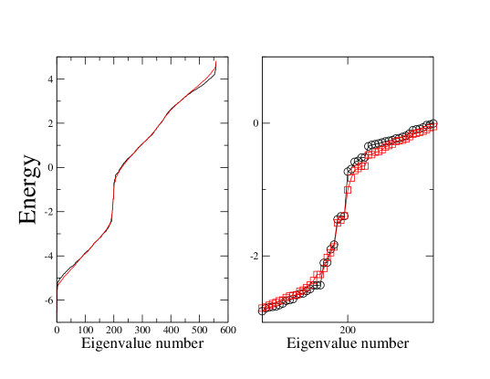
Figure 5.1. Spectrum of the Hamiltonian for $\delta=0$ (black line) and $\delta=1$ (red line). The right column is a detail of the figure near the band gap.

Diagonalization of the Hamiltonian for $\delta=0,1$ gave the energy spectra shown in Fig. (5.1). Note that for $\delta=0$ there are very few eigenvalues between roughly $-2.3$ and $-0.3$ and there are no eigenvalues between $-1.3994$ and $-0.7296$. It is important to understand that the term “band gap” can be used in two different ways in physics. One way means that there is an interval $(E_{min},E_{max})$ containing no eigenvalues. This is referred to as a “strict band gap.” The other use is that there is an interval containing very few eigenvalues, with the corresponding eigenvectors being localized. Such eigenvectors are referred to as “mid-gap states.” If there is a strict gap in the spectrum of $H$, of order unity, and if the range of $H$ is much less than unity (for example, $0.07$) in our case, then the gap can be used to prove that $P$ approximately commutes with $\hat{X},\hat{Y},\hat{Z}$ as discussed above. In the example we considered, however, there is not a very large strict band gap: if we want to consider that the energy $1$ lies in the middle of a strict band gap, then all we can say is that there are are no eigenvalues in the interval $(-1.3994,-0.7296)$. However, even without a large strict band gap, if the mid-gap states are indeed localized, then the projector $P$ will still approximately commute with $\hat{X},\hat{Y},\hat{Z}$ and so the commutators of $P\hat{X}P,P\hat{Y}P,P\hat{Z}P$ will still be small. We will see numerically below that this is the case for our problem.

There are $200$ eigenvalues less than $-1$, so the projector $P$ onto states with energy less than $-1$ has rank $200$. We computed the spectrum of $B$ for matrices $P\hat{X}P,P\hat{Y}P,P\hat{Z}P$. The index was equal to unity, so that there were $201$ eigenvalues close to unity and $199$ close to zero. The smallest eigenvalue close to unity was equal to $0.9763$ and the largest eigenvalue close to zero was equal to $0.0146$, so that there is a very clear separation between the eigenvalues close to zero and those close to unity. The largest commutator was $[P\hat{Y}P,P\hat{Z}P]$, with $\|[P\hat{Y}P,P\hat{Z}P]\|\approx 0.0298021$. Thus, the matrices are very close to commuting as claimed. In Fig. (5.2) we plot the eigenvalues of $B$.

Figure 5.2. Spectrum of $B$ for $\delta=0$, projecting onto energies above $1$. The left and right columns plot the eigenvalues close to unity and to zero, respectively. There are $201$ eigenvalues on the left and $199$ on the right.

The case with $\delta=1$ was similar. There were, in this case, $201$ eigenvalues less than $-1$ (so one eigenvalue crossed unity at some value of $\delta$ between $0$ and $1$). However, the index remained equal to unity, and the smallest eigenvalue of the $B$ close to unity was $0.9642$ while the largest eigenvalue close to zero was $0.0242$. The largest commutator was again $[P\hat{Y}P,P\hat{Z}P]$, with $\|[P\hat{Y}P,P\hat{Z}P]\|\approx 0.036728$. Thus, the matrices are very still close to commuting.

We can explicitly check that the index is insensitive to small changes in the energy as long as we do not enter the band of delocalized states. Projecting instead onto eigenvalues less than $-2$, there are a total of $195$ states, the index is still equal to unity, and the eigenvalues of $B$ which were closest to $0.5$ were $0.305$ and $0.9562$. Projecting onto eigenvalues less than $-3$, there are a total of $163$ states, the index is still equal to unity, and the eigenvalues of $B$ which were closest to $0.5$ were $0.3571$ and $0.6123$. Projecting onto eigenvalues less than $-4$, there are a total of $90$ states, the index is now equal to zero, and the eigenvalues of $B$ which were closest to $0.5$ were $0.4555$ and $0.6657$. Thus, as expected, when we move away from the band gap, the index ceases to be well-defined since the matrices cease to approximately commute.

Finally, we can check that we approximately represent the sphere, namely that $P\hat{X}P^{2}+P\hat{Y}P^{2}+P\hat{Z}P^{2}$ is close to the identity in the subspace projected onto by $P$. The smallest eigenvalue was $0.934833$ when projecting onto states with energy less than $-1$ and the $85$-th largest eigenvalue was still greater than $0.99$, but the smallest eigenvalue was only $0.447221$ when projecting onto states with energy less than $-4$.

5.4. Relation to Hall Conductance

The index calculated numerically for the lattice Hall system above is clearly closely related to the Hall conductance. The formula in lemma (3.4) expresses an approximation to the index in terms of a trace ${\rm Tr}(P\hat{X}P[P\hat{Y}P,P\hat{Z}P])$. Consider a family of Hamiltonians $H$ with increasing $L$, with a uniform lower bound on the spectral gap, and uniform upper bound on $v_{LR}$. Suppose that the dimension of the Hamiltonians, $n$, is proportional to $L^{2}$, as is natural for a two-dimensional system. Then, by lemma (5.1), the matrices $H_{r}$ form a $\delta$-representation of the sphere, with $n\delta^{2}\propto 1/L^{2}$. This means that, by lemma (3.4), ${\rm Tr}(P\hat{X}P[P\hat{Y}P,P\hat{Z}P])$ is within $1/L^{2}$ of an integer. That is, this trace is approximately quantized.

This trace is closely related to the Kubo linear response formula for the Hall effect: consider applying an electric potential to the sphere which varies uniformly between the north and south poles. This amounts to adding a term $\Psi^{\dagger}\hat{Z}\Psi$ to the Hamiltonian. If the Hall conductance is positive, this will drive a current in the counterclockwise direction around the sphere (and in the clockwise direction for negative Hall conductance). Thus, at positive $x$-coordinate, one would expect to see a current in the positive $y$-direction, and at negative $x$-coordinate one would expect to see a current in the negative $y$-direction. If the Hamiltonian $H$ is proportional to a projector, then this response is proportional to the trace ${\rm Tr}(P\hat{X}P[P\hat{Y}P,P\hat{Z}P])$, up to numeric constants, and factors of the electric charge. Thus, we prove approximate quantization of the Hall conductance in spherical geometry for non-interacting electrons for such Hamiltonians which are proportional to projectors. Perhaps with more work it will be possible in this way to prove quantization of the Hall conductance in spherical geometry for non-interacting electrons for arbitrary gapped Hamiltonians.

6. Matrices With Additional Reality Constraints

In this section, we consider further the case in which the matrices $H_{r}$ are assumed to be either real or self-dual. By the results above, since the index vanishes in this case, it is possible to approximate almost commuting real or self-dual matrices by exactly commuting matrices. However, we can ask a further question: is it possible to approximate real or self-dual matrices by exactly commuting real or self-dual matrices?

We begin with physical motivation for considering this problem. Based on the physical intuition, it is natural to conjecture that there is a $Z_{2}$ obstruction to approximating almost commuting self-dual matrices by exactly commuting self-dual matrices, and that there are no other constructions. We then verify one of these conjectures: we construct this $Z_{2}$ index, prove that if the index is nontrivial then there is a lower bound on the distance to exactly commuting self-dual matrices, and construct an example with a nontrivial index. We then finish with precise statements of our other conjectures.

6.1. Physical Motivation

In case the Hamiltonian ${\mathcal{H}}$ has time reversal symmetry, the matrix $P$ will have the same symmetry. The possible cases of interest correspond to different universality classes in random matrix theories. We discuss three classes here, corresponding to the GUE, GOE, and GSE classes. For previous application of these universality classes to classifying different insulating phases of free fermions, see [38], in particular table II.

In the GUE case, ${\mathcal{H}}$ has no time reversal symmetry, $P$ is a Hermitian projector, and $H_{r}$ are Hermitian matrices with no further symmetry constraints. In the GOE case, ${\mathcal{H}}$ has time reversal symmetry, and the time reversal symmetry operator squares to unity: this describes a spin-$0$ particle in a time reversal symmetric situation, or a spin-$1/2$ particle with time reversal symmetry and no spin-orbit coupling. In this case, $H_{r}$ are real, symmetric matrices. In the GSE case, ${\mathcal{H}}$ has time reversal symmetry, and the time reversal symmetry operator squares to minus one. This describes a spin-$1/2$ particle with strong spin-orbit coupling. In this case, the $H_{r}$ are self-dual.

In the GSE case, the index vanishes due to the time reversal symmetry as explained above. There is therefore no index obstruction to approximating $H_{r}$ by exactly commuting $H_{r}^{\prime}$. However, it is natural to look for a $Z_{2}$ obstruction to approximating three almost commuting $H_{r}$ by self-dual $H_{r}^{\prime}$, because we know that there is a $Z_{2}$ index characterizing different translationally invariant phases of free fermions with symplectic symmetry in two dimensions [25, 24]. Such topologically nontrivial phases are expected, by their nature, to be stable to perturbations of the Hamiltonian which break translational symmetry, as discussed in [38] and have been observed experimentally in $HgTe/(Hg,Ce)Te$ quantum wells[27].

6.2. Index Obstruction

We construct the index by finding a unitary transformation that makes $S(H_{1},H_{2},H_{3})$ anti-symmetric and then taking the sign of the Pfaffian of this matrix. From a physical point of view, the existence of this unitary transformation is not surprising: the self-dual operation can be regarded as a time-reversal symmetry operation, and a similar time-reversal symmetry can be applied to the $\sigma$ matrices used to construct $S(H_{1},H_{2},H_{3})$. Under these combined time reversal symmetries, $S(H_{1},H_{2},H_{3})$ changes sign; however, since there are two spin-$1/2$s, the time reversal symmetry operator squares to unity and hence, up to a basis change, is equivalent to transposition. We now show this.

Lemma 6.1.

Let $H_{r}$ be self-dual. Define the matrix $\tilde{B}(H_{1},H_{2},H_{3})$ by

(6.1) $$\tilde{B}(H_{1},H_{2},H_{3})=U^{*}S(H_{1},H_{2},H_{3})U,$$

where the unitary $U$ is defined by

(6.2) $$U=\frac{1}{\sqrt{2}}(I+Z\otimes\sigma_{2}).$$

Then, the matrix $\tilde{B}$ is anti-symmetric.

Proof.

Note that for any $r$, $\sigma_{r}^{T}=-\sigma_{2}\sigma_{r}\sigma_{2}$, while $H_{r}^{T}=-ZH_{r}Z$, by the assumption of self-duality. Also, $U^{T}=U$. Thus,

$$\tilde{B}(H_{1},H_{2},H_{3})^{T} = US(H_{1},H_{2},H_{3})^{T}U^{*}$$

$$= U\Bigl{(}\sum_{r}H_{r}\otimes\sigma_{r}\Bigr{)}^{T}U^{*}$$

$$= U\Bigl{(}\sum_{r}H_{r}^{T}\otimes\sigma_{r}^{T}\Bigr{)}U^{*}$$

$$= U\Bigl{(}\sum_{r}ZH_{r}Z\otimes\sigma_{2}\sigma_{r}\sigma_{2}\Bigr{)}U^{*}$$

$$= U\Bigl{(}Z\otimes\sigma_{2}\Bigr{)}\Bigl{(}\sum_{r}H_{r}\otimes\sigma_{r}\Bigr{)}\Bigl{(}Z\otimes\sigma_{2}\Bigr{)}U^{*}.$$

Note that $(Z\otimes\sigma_{2})^{2}=-I$, so

$$U\Bigl{(}Z\otimes\sigma_{2}\Bigr{)} = -\frac{1}{\sqrt{2}}(I-Z\otimes\sigma_{2})$$

$$= -U^{*},$$

and

$$\Bigl{(}Z\otimes\sigma_{2}\Bigr{)}U^{*} = \frac{1}{\sqrt{2}}(I+Z\otimes\sigma_{2})U^{*}$$

$$= U.$$

Thus,

$$U\Bigl{(}Z\otimes\sigma_{2}\Bigr{)}\Bigl{(}\sum_{r}H_{r}\otimes\sigma_{r}\Bigr{)}\Bigl{(}Z\otimes\sigma_{2}\Bigr{)}U^{*} = -U^{*}\Bigl{(}\sum_{r}H_{r}\otimes\sigma_{r}\Bigr{)}U$$

$$= -\tilde{B}(H_{1},H_{2},H_{3}).$$

∎

Definition 6.2.

We define the index $\widetilde{\rm bott}(H_{1},H_{2},H_{3})$ for self-dual matrices $H_{r}$ by

(6.7) $$\widetilde{\rm bott}(H_{1},H_{2},H_{3})={\rm sgn}({\rm Pf}(\tilde{B}(H_{1},H_{2},H_{3}))),$$

where ${\rm Pf}$ is the Pfaffian and ${\rm sgn}(x)=1$ for $x>0$ and ${\rm sgn}(x)=-1$ for $x<0$. If ${\rm Pf}(\tilde{B}(H_{1},H_{2},H_{3}))=0$, the index $\widetilde{\rm bott}(H_{1},H_{2},H_{3})$ is not defined.

Lemma 6.3.

Consider any continuous path of self-dual matrices, $H_{r}(s)$, where $s$ is a real number, $0\leq s\leq 1$. Suppose that for all $s$, the matrix $B(H_{1},H_{2},H_{3})$ has non-vanishing determinant. Then, $\widetilde{\rm bott}(H_{1}(0),H_{2}(0),H_{3}(0))=\widetilde{\rm bott}(H_{1}(1),H_{2}(1),H_{3}(1))$.

Proof.

The determinant of $B(H_{1},H_{2},H_{3})$ is equal to ${\rm Pf}(\tilde{B}(H_{1},H_{2},H_{3}))^{2}$. As long as the determinant does not vanish, the Pfaffian does not vanish and hence cannot change sign. ∎

Lemma 6.4.

If $H_{1},H_{2},H_{3}$ are self-dual and exactly commuting and $\widetilde{\rm bott}(H_{1},H_{2},H_{3})$ is defined, then $\widetilde{\rm bott}(H_{1},H_{2},H_{3})=1$.

Proof.

Note that $\widetilde{\rm bott}$ is multiplicative under direct sum of matrices. Also, $\widetilde{\rm bott}$ is invariant under symplectic transformation of the $H_{r}$ (these transformations preserve the property of being self-dual). Finally, for any commuting self-dual matrices $H_{r}$, we can find a symplectic transformation which makes the $H_{r}$ diagonal; the diagonal entries of these matrices come in pairs which are equal. That is, if the $H_{r}$ are $2n$ dimensional matrices, then after this symplectic transformation then each $H_{r}$ is equal to the direct sum of $n$ different $2$-by-$2$ matrices which are proportional to the identity. Thus, it suffices to consider the case in which the $H_{r}$ are real scalar multiples of the $2$-by-$2$ identity matrix. If $H_{r}=\alpha_{r}I$ then

$$\tilde{B}(H_{1},H_{2},H_{3}) = \frac{1}{2}(I-Z\otimes\sigma_{2})\Bigl{(}\sum\alpha_{r}\otimes\sigma_{r}\Bigr{)}(I+Z\otimes\sigma_{2})$$

$$= i\alpha_{3}Z\otimes\sigma_{3}+i\alpha_{2}I\otimes\sigma_{2}+i\alpha_{3}Z\otimes\sigma_{1}$$

$$= \begin{pmatrix}0&i\alpha_{1}&i\alpha_{2}&i\alpha_{3}\\ -i\alpha_{1}&0&-i\alpha_{3}&i\alpha_{2}\\ i\alpha_{2}&i\alpha_{3}&0&-i\alpha_{1}\\ -i\alpha_{3}&i\alpha_{2}&i\alpha_{1}&0\end{pmatrix}$$

This matrix has Pfaffian equal to

$$(i\alpha_{1})(-i\alpha_{1})-(i\alpha_{2})(i\alpha_{2})+(i\alpha_{3})(-i\alpha_{3})=\alpha_{1}^{2}+\alpha_{2}^{2}+\alpha_{3}^{2}.$$

∎

We now show that for any $\delta>0$, there exist self-dual matrices $H_{r}$ which form a $\delta$-representation of the sphere with $\widetilde{\rm bott}(H_{1},H_{2},H_{3})=-1$. This example essentially consists of two copies of the matrices in (1.2), with opposite Bott index between the two copies.

Example 6.5.

Let $n=2S+1.$ Consider the spin matrices $S^{1},S^{2},S^{3}$ for a quantum spin $S$ with $H_{1}=I^{(1)}\otimes S^{1}/\sqrt{S(S+1)}$, $H_{2}=\sigma_{2}^{(1)}\otimes S^{2}/\sqrt{S(S+1)}$, $H_{3}=I^{(1)}\otimes S^{3}/\sqrt{S(S+1)}$. We will be using the $\sigma$ matrices in two different ways in this example: first, to form the $2n$ dimensional matrices $H_{r}$ from the $n$ dimensional matrices $S^{r}$, second to form the matrix $\tilde{B}$. We use $\sigma^{(1)}$ to refer to the first case, and $\sigma^{(2)}$ to refer to the second. Note that $Z=-i\sigma_{2}^{(1)}\otimes I$. We use $I^{(1)}$ to refer to the $2$-by-$2$ identity matrix. The matrix $S^{2}$ is anti-symmetric, while $S^{1},S^{3}$ are symmetric.

It is easy to see that

$$\|H_{r},H_{s}\|\leq 1/S,$$

so that the matrices form a $\delta$-representation of the sphere with $\delta=1/S$.

We claim that $\widetilde{\rm bott}(H_{1},H_{2},H_{3})=-1$.

Proof.

We now compute the Pfaffian. Since the index depends only on the sign of the Pfaffian, we ignore constant factors which are real and positive. We have

$$\tilde{B}(H_{1},H_{2},H_{3})$$

$$= {\rm const.}\times(I-Z\otimes\sigma^{(2)}_{2})B(H_{1},H_{2},H_{3})(I+Z\otimes\sigma^{(2)}_{2})$$

$$= {\rm const.}\times\sigma^{(1)}_{2}\otimes\Bigl{(}S^{x}\otimes\sigma^{(2)}_{3}+S^{y}\otimes\sigma^{(2)}_{2}-S^{z}\otimes\sigma^{(2)}_{1}\Bigr{)}.$$

Unitarily conjugate this matrix $\tilde{B}(H_{1},H_{2},H_{3})$ by the orthogonal transformation $(1/\sqrt{2})I\otimes(I^{(2)}+i\sigma^{(2)}_{2})$, giving the matrix ${\rm const.}\times\sigma^{(1)}_{2}\otimes\sum_{r}S^{r}\sigma^{(2)}_{r}$. Since this orthogonal transformation has determinant $+1$, the Pfaffian is unchanged.

The matrix $\sigma^{(1)}_{2}\otimes\sum_{r}S^{r}\sigma^{(2)}_{r}$ is anti-symmetric and equals

(6.10) $$\begin{pmatrix}0&i\sum_{r}S^{r}\sigma_{r}\\ -i\sum_{r}S^{r}\sigma_{r}&0\end{pmatrix}$$

The Pfaffian of this matrix is equal to the determinant of $i\sum_{r}S^{r}\sigma_{r}$, which is equal to $i^{4S+2}$ times the determinant of $\sum_{r}S^{r}\sigma_{r}$. The matrix $\sum_{r}S^{r}\sigma_{r}$ has $2(S+1/2)+1=2S+2$ positive eigenvalues and $2(S-1/2)+1=2S$ negative eigenvalues, as computed in example (1.2). Thus, the sign of the Pfaffian is equal to

(6.11) $$i^{4S+2}(-)^{2S}=-1.$$

∎

Lemma 6.6.

Suppose $\left(H_{1},H_{2},H_{3}\right)$ and $\left(K_{1},K_{2},K_{3}\right)$ are triples of self-dual, Hermitian $n$-by-$n$ matrices and suppose $\left(H_{1},H_{2},H_{3}\right)$ is a $\delta$-representation of the sphere with $\delta<1/4$. If

$$\left\|H_{1}-K_{1}\right\|+\left\|H_{2}-K_{2}\right\|+\left\|H_{3}-K_{3}\right\|\leq\sqrt{1-4\delta}$$

then

$$\widetilde{\rm bott}(K_{1},K_{2},K_{3})=\widetilde{\rm bott}(H_{1},H_{2},H_{3})$$

Proof.

We showed in the proof of Lemma 3.5 that the line segment from $S(H_{1},H_{2},H_{3})$ to $S(K_{1},K_{2},K3)$ passes through invertibles. It follows that the line segment from $\tilde{B}(H_{1},H_{2},H_{3})$ to $\tilde{B}(K_{1},K_{2},K3)$ passes through skew-symmetric invertibles and so by lemma (6.3) the Pfaffian does not change sign. ∎

As a corollary, the distance in operator norm from the matrices in Example (6.5) to the nearest exactly commuting triple of self-dual matrices is at least $\sqrt{1-4/S}$.

6.3. Conjectures

We believe that the absence of this index obstruction implies that is possible to approximate almost commuting self-dual matrices by exactly commuting self-dual matrices. Before addressing this issue, we need to understand the two matrix case in the presence of additional symmetry. We thus raise the following conjectures which generalize Lin’s theorem:

Conjecture 1.

For all $\epsilon>0$, there exists a $\delta>0$ such that, given any real, symmetric matrices $A,B$ with $\|[A,B]\|\leq\delta$ and $\|A\|,\|B\|\leq 1$, there exist real, symmetric matrices $A^{\prime},B^{\prime}$, with $[A^{\prime},B^{\prime}]=0$ and $\|A-A^{\prime}\|,\|B-B^{\prime}\|\leq\epsilon$.

Conjecture 2.

For all $\epsilon>0$, there exists a $\delta>0$ such that, given any self-dual, Hermitian matrices $A,B$ with $\|[A,B]\|\leq\delta$ and $\|A\|,\|B\|\leq 1$, there exist self-dual, Hermitian matrices $A^{\prime},B^{\prime}$, with $[A^{\prime},B^{\prime}]=0$ and $\|A-A^{\prime}\|,\|B-B^{\prime}\|\leq\epsilon$.

The conjectures we make regarding index obstructions are:

Conjecture 3.

For all $\epsilon>0$, there exists a $\delta>0$ such that, given any real, symmetric matrices $H_{1},H_{2},H_{3}$ with $\|[H_{1},H_{2}]\|,\|[H_{2},H_{3}]\|,\|[H_{3},H_{1}]\|\leq\delta$, and

(6.12) $$H_{1}^{2}+H_{2}^{2}+H_{3}^{2}=I,$$

there exist real, symmetric commuting matrices $H_{1}^{\prime},H_{2}^{\prime},H_{3}^{\prime}$, with $\|H_{1}-H_{1}^{\prime}\|,\|H_{2}-H_{2}^{\prime}\|,\|H_{3}-H_{3}^{\prime}\|\leq\epsilon$.

Conjecture 4.

For all $\epsilon>0$, there exists a $\delta>0$ such that, given any self-dual Hermitian matrices $H_{1},H_{2},H_{3}$ with $\widetilde{\rm bott}(H_{1},H_{2},H_{3})=1$ and $\|[H_{1},H_{2}]\|,\|[H_{2},H_{3}]\|,\|[H_{3},H_{1}]\|\leq\delta$, and

(6.13) $$H_{1}^{2}+H_{2}^{2}+H_{3}^{2}=I,$$

there exist self-dual Hermitian commuting matrices $H_{1}^{\prime},H_{2}^{\prime},H_{3}^{\prime}$, with $\|H_{1}-H_{1}^{\prime}\|,\|H_{2}-H_{2}^{\prime}\|,\|H_{3}-H_{3}^{\prime}\|\leq\epsilon$.

7. Discussion

We have given quantitative error bounds on the ability to approximate three almost commuting matrices by three exactly commuting matrices under the assumption of a vanishing index assumption. We have related the ability to approximate these matrices to the ability to find localized Wannier functions in a physical system, and we have demonstrated that it is readily possible to numerically calculate this index for such systems.

We have constructed a $Z_{2}$ index obstruction to approximation of almost commuting self-dual matrices by exactly commuting self-dual matrices, and raised additional conjectures regarding almost commuting matrices in the case of real $C^{*}$-algebras. Finally, we note that table II of [38] lists $10$ different classes of matrices and different index possibilities in various dimensions. We believe more generally that each of the obstructions in $d=2$ in this table will correspond to a particular obstruction to approximating almost commuting matrices; i.e., we expect that for almost commuting matrices in class DIII there will be a $Z_{2}$ obstruction to approximating them by exactly commuting matrices of class DIII. Such obstruction is left for future work.

References

• [1] J. E. Avron and R. Seiler. Quantization of the hall conductance for general multiparticle schrodinger operators. Phs. Rev. Lett., 54:259, 1985.
• [2] J. Bellissard, A. van Elst, and H. Schulz-Baldes. The noncommutative geometry of the quantum Hall effect. J. Math. Phys., 35(10):5373–5451, 1994.
• [3] Rajendra Bhatia and Fuad Kittaneh. Some inequalities for norms of commutators. SIAM J. Matrix Anal. Appl., 18(1):258–263, 1997.
• [4] Ola Bratteli, George A. Elliott, David E. Evans, and Akitaka Kishimoto. Homotopy of a pair of approximately commuting unitaries in a simple $C^{*}$-algebra. J. Funct. Anal., 160(2):466–523, 1998.
• [5] C. Brouder, G. Panati, M. Calandra, C. Mourougane, and Marzari N. Exponential localization of wannier functions in insulators. Phys. Rev. Lett., 98:046402, 2007.
• [6] Nathanial P. Brown. On quasidiagonal $C^{*}$-algebras. In Operator algebras and applications, volume 38 of Adv. Stud. Pure Math., pages 19–64. Math. Soc. Japan, Tokyo, 2004.
• [7] Man Duen Choi. Almost commuting matrices need not be nearly commuting. Proc. Amer. Math. Soc., 102(3):529–533, 1988.
• [8] Kenneth R. Davidson. Almost commuting Hermitian matrices. Math. Scand., 56(2):222–240, 1985.
• [9] Kenneth R. Davidson and Stanislaw J. Szarek. Local operator theory, random matrices and Banach spaces. In Handbook of the geometry of Banach spaces, Vol. I, pages 317–366. North-Holland, Amsterdam, 2001.
• [10] Søren Eilers, Terry A. Loring, and Gert K. Pedersen. Morphisms of extensions of $C^{*}$-algebras: pushing forward the Busby invariant. Adv. Math., 147(1):74–109, 1999.
• [11] George A. Elliott and Mikael Rørdam. Classification of certain infinite simple $C^{*}$-algebras. II. Comment. Math. Helv., 70(4):615–638, 1995.
• [12] Ruy Exel. The soft torus and applications to almost commuting matrices. Pacific J. Math., 160(2):207–217, 1993.
• [13] Ruy Exel and Terry Loring. Almost commuting unitary matrices. Proc. Amer. Math. Soc., 106(4):913–915, 1989.
• [14] Ruy Exel and Terry A. Loring. Invariants of almost commuting unitaries. J. Funct. Anal., 95(2):364–376, 1991.
• [15] Guihua Gong and Huaxin Lin. Almost multiplicative morphisms and almost commuting matrices. J. Operator Theory, 40(2):217–275, 1998.
• [16] Don Hadwin. Strongly quasidiagonal $C^{*}$-algebras. J. Operator Theory, 18(1):3–18, 1987. With an appendix by Jonathan Rosenberg.
• [17] Paul R. Halmos. Finite-dimensional vector spaces. Springer-Verlag, New York, second edition, 1974. Undergraduate Texts in Mathematics.
• [18] M. B. Hastings. Making almost commuting matrices commute. Communications in Mathematical Physics, 291(2):321–345, 2009.
• [19] Matthew B. Hastings and Tohru Koma. Spectral gap and exponential decay of correlations. Comm. Math. Phys., 265(3):781–804, 2006.
• [20] MB Hastings. Lieb-Schultz-Mattis in higher dimensions. Physical Review B, 69(10):104431, 2004.
• [21] MB Hastings. Locality in quantum and Markov dynamics on lattices and networks. Physical review letters, 93(14):140402, 2004.
• [22] MB Hastings et al. Topology and phases in fermionic systems. J. Stat. Mech, page L01001, 2008.
• [23] Richard V. Kadison and John R. Ringrose. Fundamentals of the theory of operator algebras. Vol. I, volume 100 of Pure and Applied Mathematics. Academic Press Inc. [Harcourt Brace Jovanovich Publishers], New York, 1983. Elementary theory.
• [24] CL Kane and EJ Mele. Quantum spin Hall effect in graphene. Physical review letters, 95(22):226801, 2005.
• [25] CL Kane and EJ Mele. Z_ $\{$2$\}$ Topological Order and the Quantum Spin Hall Effect. Physical review letters, 95(14):146802, 2005.
• [26] Alexei Kitaev. Periodic table for topological insulators and superconductors. http://arxiv.org/abs/0901.2686, to appear in the Proceedings of the L.D.Landau Memorial Conference "Advances in Theoretical Physics", June 22-26, 2008, Chernogolovka, Moscow region, Russia, 2009.
• [27] M. Konig, S. Wiedmann, C. Brune, A. Roth, H. Buhmann, L.W. Molenkamp, X.L. Qi, and S.C. Zhang. Quantum spin Hall insulator state in HgTe quantum wells. Science, 318(5851):766, 2007.
• [28] W. Li. On the perturbation bound in unitarily invariant norms for subunitary polar factors. Linear Algebra and Its Applications, 429(2-3):649–657, 2008.
• [29] Elliott H. Lieb and Derek W. Robinson. The finite group velocity of quantum spin systems. Comm. Math. Phys., 28:251–257, 1972.
• [30] Huaxin Lin. Almost commuting selfadjoint matrices and applications. In Operator algebras and their applications (Waterloo, ON, 1994/1995), volume 13 of Fields Inst. Commun., pages 193–233. Amer. Math. Soc., Providence, RI, 1997.
• [31] Huaxin Lin. Almost commuting unitaries and classification of purely infinite simple $C^{*}$-algebras. J. Funct. Anal., 155(1):1–24, 1998.
• [32] Terry A. Loring. The torus and noncommutative topology. PhD thesis, University of California, Berkeley, 1986.
• [33] Terry A. Loring. $K$-theory and asymptotically commuting matrices. Canad. J. Math., 40(1):197–216, 1988.
• [34] Terry A. Loring. When matrices commute. Math. Scand., 82(2):305–319, 1998.
• [35] Bruno Nachtergaele and Robert Sims. Lieb-Robinson bounds and the exponential clustering theorem. Comm. Math. Phys., 265(1):119–130, 2006.
• [36] T.J. Osborne. Almost commuting unitaries with spectral gap are near commuting unitaries. Proc. Amer. Math. Soc., 137:4043–4048, 2009.
• [37] Gert K. Pedersen. A commutator inequality. In Operator algebras, mathematical physics, and low-dimensional topology (Istanbul, 1991), volume 5 of Res. Notes Math., pages 233–235. A K Peters, Wellesley, MA, 1993.
• [38] A.P. Schnyder, S. Ryu, A. Furusaki, and A.W.W. Ludwig. Classification of Topological Insulators and Superconductors. In AIP Conference Proceedings, volume 1134, page 10, 2009.
• [39] Dan Voiculescu. Asymptotically commuting finite rank unitary operators without commuting approximants. Acta Sci. Math. (Szeged), 45(1-4):429–431, 1983.
• [40] Dan Voiculescu. Around quasidiagonal operators. Integral Equations Operator Theory, 17(1):137–149, 1993.