Determination of $B_{K}$ using improved staggered fermions (II) SU(2) chiral perturbation theory fit

Abstract:

We present results for $B_{K}$ calculated using HYP-smeared improved staggered fermions on the MILC asqtad lattices. In this report, the data is analyzed using the results of SU(2) staggered chiral perturbation theory (SChPT). We outline the derivation of the NLO SU(2) SChPT result, explain our fitting procedure, and outline how we estimate systematic errors. We also show the light sea-quark mass and lattice spacing dependence for both SU(2) and SU(3)-based analyses. Our preliminary result from the SU(2) analysis is $B_{K}(\text{NDR},\mu=2\text{ GeV})=0.512\pm 0.014\pm 0.034$ and $\hat{B}_{K}=B_{K}(\text{RGI})=0.701\pm 0.019\pm 0.047$. This is somewhat more accurate than our result from the SU(3) analysis. It is consistent with results obtained using valence domain-wall fermions.

1 Introduction

This paper is the second in a series of the four proceedings describing our calculation of $B_{K}$. In the first, we provided a brief phenomenological introduction, outlined the results of SU(3) staggered chiral perturbation theory (SChPT), and explained the corresponding fitting strategy [1]. Here, we explain briefly how we obtain the SU(2) SChPT result, outline how we use this result to analyze our data, and present a preliminary value, and error budget, for $B_{K}$. The details of the lattice ensembles and quark masses are as in Ref. [1].

The use of SU(2) ChPT was pioneered in the lattice context by the RBC collaboration [2]. One treats kaons and $\eta$’s as heavy, static sources for pseudo-Goldstone bosons (PGBs) composed of light quarks (the “pions”). Unlike the SU(3) version, SU(2) ChPT does not require an expansion in the ratio $r_{s}=m_{s}/\Lambda_{\rm QCD}$. The expansion parameter is thus $r_{l}=m_{\ell}/\Lambda_{\rm QCD}$ (with $m_{\ell}$ the common up and down quark mass in our isospin-symmetric simulations). This improves convergence properties (as long as $m_{\ell}$ is light enough), although this comes at a price: one fits to a smaller number of data-points, and must do so with low-energy coefficients (LECs) that have an unknown, analytic dependence on $m_{s}/\Lambda_{\rm QCD}$.

Our calculations have valence quark masses ranging from approximately $m_{s}^{\rm phys}/10$ to $m_{s}^{\rm phys}$. Despite the large upper value, we find that SU(3) fits give a reasonable description of our data. The main problem is the presence of multiple contributions to the NLO formula arising from discretization errors or from truncation of the perturbative matching factors. These lattice artefacts are poorly determined in the fits and lead to $\sim 5\%$ uncertainties upon extrapolation to the physical light-quark mass. A major advantage of the SU(2) approach in our context is that all these artefacts are moved to NNLO, i.e. are known to be very small. This allows a better-controlled extrapolation to the physical mass.

2 SU(2) Staggered ChPT Analysis

The following description is necessarily very brief. A full explanation will appear in Ref. [3].

We need to generalize the SU(2) result for $B_{K}$ given in continuum ChPT in Ref. [2] to include the artefacts associated with staggered fermions. This generalization has been done in the SU(3) case in Ref. [4], but requires a rather involved operator enumeration. Rather than carry out a direct generalization to SU(2) SChPT, we instead have worked to all orders in $r_{s}$ (though to NLO in $r_{\ell}$) within SU(3) SChPT. Using power-counting arguments, we find a simple result [3]: one can obtain the NLO SU(2) SChPT result simply by taking the SU(2) limit of the NLO SU(3) SChPT result, and then allowing (almost) all of the LECs to have an unknown dependence on $r_{s}$. The only exception to this arbitrary dependence is the factor of $1/f_{\pi}^{2}$ multiplying the pion chiral logarithms, which remains unchanged.

Applying this result we find the simplification noted above, namely that all the non-analytic contributions multiplied by LECs proportional to $a^{2}$ or $\alpha^{2}$ are pushed to NNLO in SU(2) SChPT. This happens because the factor of $M_{K}^{2}$ in the numerator of $B_{K}$ is balanced by a chiral logarithm proportional to $M_{\pi}^{2}\log(M_{\pi})$. In SU(3) ChPT this ratio is of $O(1)$, but in the SU(2) case it is of NLO. The overall factor of $a^{2}$ or $\alpha^{2}$ then moves the term to NNLO.

The final result is that taste-breaking effects only enter the NLO expression through the masses of the pions of different tastes. The predicted form is

$$f_{\text{th}} = d_{0}F_{0}+d_{1}\frac{X_{P}}{\Lambda_{\chi}^{2}}+d_{2}\frac{X_{P}^{2}}{\Lambda_{\chi}^{4}}+d_{3}\frac{L_{P}}{\Lambda_{\chi}^{2}}$$ (1)

where the chiral logarithms (defined in Ref. [1]) reside in the function

$$F_{0} = 1+\frac{1}{32\pi^{2}f_{\pi}^{2}}\Big{\{}\ell(X_{\textrm{I}})+(L_{\textrm{I}}-X_{\textrm{I}})\tilde{\ell}(X_{\textrm{I}})-2\langle\ell(X_{\textrm{B}})\rangle\Big{\}}$$ (2)

$$\langle\ell(X_{\textrm{B}})\rangle = \frac{1}{16}\Big{[}\ell(X_{\textrm{I}})+\ell(X_{\textrm{P}})+4\ell(X_{\textrm{V}})+4\ell(X_{\textrm{A}})+6\ell(X_{\textrm{T}})\Big{]}\,.$$ (3)

Here $X_{\textrm{B}}$ ($L_{\textrm{B}}$) is the squared mass of the valence (sea) pion with taste B, which we know from our simulations or those of the MILC collaboration. The scale $\Lambda_{\chi}$ is arbitrary and we take it to be 1 GeV. The coefficients $d_{i}$ have an unknown dependence on $r_{s}$, and, in addition, at NLO $d_{0}$ depends also on $a^{2}$ and $\alpha^{2}$.

As for SU(3) fitting, we include a single analytic NNLO term—that proportional to $d_{2}$. In the SU(2) case, however, we find that we can drop this term if we consider only the smallest valence light-quark masses. In the following we label such fits as “NLO”, while if we include the $d_{2}$ term we label the fits with “NNLO”.

3 SU(2) SChPT Fitting

A major advantage of the SU(2) analysis is that the fitting function is much simpler than that for SU(3). As a consequence, we do not need to include Bayesian priors for any of the parameters.

Our choice of which valence quark masses to include in the analysis is exemplified by our approach on the coarse MILC lattices ($a\approx 0.12\;$fm). Here the physical strange quark mass is $am^{\textrm{phy}}_{s}\cong 0.052$, and we choose the nearest three values for the valence strange-quark mass, $am_{y}=\{0.05,0.045,0.04\}$, in order to extrapolate to the physical value. For the valence down-quark mass we use our lightest four values, $am_{x}=\{0.005,0.01,0.015,0.02\}$, to extrapolate to $am_{d}^{\rm phys}$. These choices ensure that the expansion parameter of SU(2) ChPT is relatively small: $m_{x}/m_{y}\leq 1/2$. Analogous choices of quark masses are made on the fine and superfine ensembles [3]. We call this choice “4X3Y”, and use it for our central value. We have also considered “5X3Y” fits.

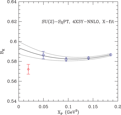
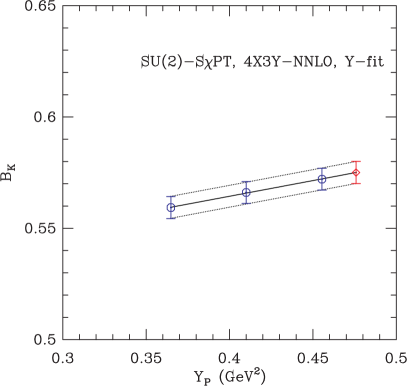
Figure 1: One-loop matched $B_{K}$ fitted versus $X_{P}$ (left) and $Y_{P}$ (right), on the MILC coarse lattices with $am_{\ell}=0.01$ and $am_{s}=0.05$. In the left panel $am_{y}=0.05$, and the (red) diamond shows the result after removing lattice artefacts. The fit type is 4X3Y-NNLO. $B_{K}$ is obtained using one-loop matching. See text for more details.

In Fig. 1, we show examples of the resulting fits. In the left plot, the (blue) octagons show the one-loop matched lattice data, which are then fit to the NNLO form of eq. (1). There are only 3 parameters because $L_{P}$ is fixed in this partially-quenched fit. With the fit parameters determined, we then evaluate the expression (1) at the physical pion mass and with taste splittings set to zero, i.e with $X_{\textrm{B}}=L_{\textrm{I}}=M_{\pi}^{2}$. This removes all taste-breaking discretization and truncation errors, and results in the point shown with the (red) diamond. We call this procedure the “X-fit”, and we repeat it for each of the values of $am_{y}$.

We then proceed to the “Y-fit”, illustrated in the right panel of Fig. 1. Here we use either a linear or a quadratic fit to extrapolate the short distance to the physical value $Y_{\textrm{P}}=2M_{K}^{2}-M_{\pi}^{2}$. We find, as seen in the figure, that the dependence is weak and close to linear. Thus we use the linear fit for our central value and the quadratic fit to estimate a systematic error. In the figure, the red diamond shows the result of linear extrapolation.

4 Dependence on the Light Sea Quark Mass

After the X- and Y-fits, the resulting intermediate value for $B_{K}$ still has the analytic dependence on the light sea-quark mass $am_{l}$ (entering through the $d_{3}$ term), as well as taste-conserving discretization and truncation errors. Here, we investigate the dependence on $am_{l}\propto L_{\textrm{P}}$, which we have studied on the MILC coarse ensembles. We also discuss the corresponding dependence of the result of the SU(3) SChPT fit discussed in Ref. [1].

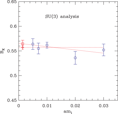
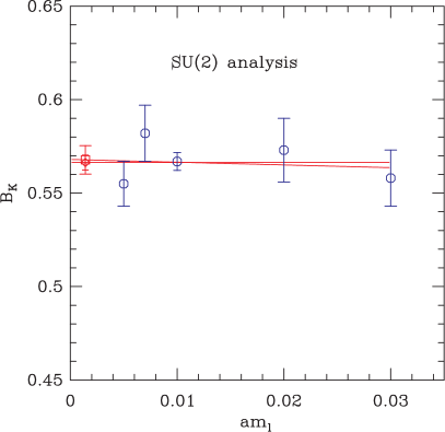
Figure 2: $B_{K}$ (after X- and Y-fitting) versus $am_{l}$ for the SU(3) analysis (left) and for the SU(2) analysis (right). Data is from the MILC coarse lattices. The fit types are N-BT7 for SU(3) and 4X3Y-NNLO for SU(2). See text for details.

In Fig. 2, we show the $am_{\ell}$ dependence for both SU(3) and SU(2) fits. We have fit to the expected linear dependence [resulting in the (red) squares], and also, since the data show very little dependence on $am_{\ell}$, to a constant [(red) diamonds].

The weakness of the dependence on $am_{\ell}$ is striking. It has the important consequence that our use of only a single light sea-quark mass on the fine and superfine lattices does not introduce a large uncertainty. We use the difference between the constant and linear fits as an estimate of the systematic error arising from the uncertainty in the $am_{\ell}$ dependence. As the figure shows, this error is somewhat smaller for SU(2) fitting than for SU(3).

5 Continuum Extrapolation

The dominant errors remaining at this stage are those due to taste-conserving discretization and truncation errors. These vary as $a^{2}\alpha^{n}$, where $n=0,1,\dots$ ($n=0$ is allowed since we do not use Symanzik-improved operators), and as $\alpha^{2}$. We cannot disentangle these effects using a fit to three lattice spacings, so proceed as follows. We fit our data to a linear function of $a^{2}$, and estimate the $O(\alpha^{2})$ truncation error separately (as described in a companion proceeding [7]). More precisely, we fit to the data from the lattices with $a=0.12,0.09,0.06\;$fm having $am_{l}/am_{s}$ fixed to $1/5$. The results for both SU(3) and SU(2) analyses are shown in Fig. 3. We use the extrapolated values for our main result, and take the difference between them and the results on the superfine lattices as an estimate of the systematic error due to the continuum extrapolation.

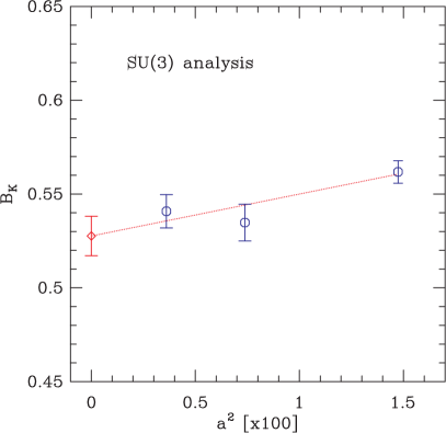
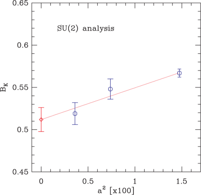
Figure 3: One-loop matched $B_{K}$ plotted versus $a^{2}$ for the SU(3) analysis (left) and for the SU(2) analysis (right). The fit types are N-BT7 for SU(3) and 4X3Y-NNLO for SU(2).

The dependence on $a^{2}$ is noticeable for both analyses, with $B_{K}$ increasing by about 6% and 10% between $a=0$ and $0.12\;$fm in the SU(3) and SU(2) cases, respectively. Assuming a form $B_{K}^{\rm cont}[1+(a\Lambda)^{2}]$ this corresponds to scales of $\Lambda\approx 400$ and $500\;$MeV. These are reasonable values, indicating that HYP-smearing has reduced the discretization errors with staggered fermions down to canonical size.

6 Error Budget and Conclusion

cause	error (%)	description
statistics	2.8	4X3Y-NNLO fit (ensemble C3)
discretization	1.4	diff. of (S1) and $a=0$
fitting (1)	0.15	X-fit: NLO vs. NNLO
fitting (2)	0.5	Y-fit: linear vs. quadratic
fitting (3)	0.25	constant vs linear $am_{l}$ dependence
finite volume	0.89	$20^{3}$ (C3) versus $28^{3}$ (C3-2)
matching factor	6.4	$\Delta B_{K}^{(2)^{\prime}}$ (S1)
$r_{1}$	0.09	uncertainty in $r_{1}$

Table 1: Preliminary error budget for $B_{K}$ obtained using SU(2) SChPT fitting.

In Table 1, we summarize our present best estimates of the uncertainties in $B_{K}$ arising from various sources. The method by which we estimate these errors is outlined in the “description”, and has in most cases been explained above. The statistical error is obtained from using a global jackknife procedure. The finite volume estimate is obtained by comparing results on two volumes, as described in one of the companion proceedings [6]. This error is comparable to that estimated using NLO ChPT. The error due to the use of one-loop matching is estimated in another of the companion proceedings [7]. The error due to the uncertainty in the scale $r_{1}$ is estimated by varying the input values within the quoted errors and repeating the analysis.

One error not included in this budget is that due to the strange sea-quark mass differing slightly from its physical value. Given the weak dependence on the light sea-quark mass, we expect this to be a negligible effect, but plan to make a more quantitative estimate in the future.

Combining these errors, our current, preliminary result for $B_{K}$ using SU(2) SChPT fitting is

$$\begin{array}[]{l l c}B_{K}(\text{NDR},\mu=2\text{ GeV})&=0.512\pm 0.014\pm 0.034&\qquad[{\rm SU(2),\ {\bf PRELIMINARY}}]\,,\\ \hat{B}_{K}=B_{K}(\text{RGI})&=0.701\pm 0.019\pm 0.047&\qquad[{\rm SU(2),\ {\bf PRELIMINARY}}]\,,\end{array}$$ (4)

where the first error is statistical and the second systematic. The total error is thus about 7%, and is dominated by the error in the matching factor. The total error is smaller than the 9% preliminary error we find for the SU(3) analysis [1]. The statistical error in the latter analysis is smaller (as can be seen in the earlier plots, and arises because there are more data points in the fits) but this is more than balanced by an increase in the systematic errors.

Our result is consistent with other $2+1$-flavor unquenched results obtained using different fermion discretizations, all of which are summarized in Ref. [8]. For example the calculation of Ref. [9] using domain-wall valence fermions on the coarse and fine MILC lattices finds $B_{K}({\rm NDR},\mu=2\;{\rm GeV})=0.527(6)(20)$. The agreement between calculations using different fermion discretizations provides a highly non-trivial cross-check on the results.

During the next year, we aim to reduce our errors by adding a fourth (“ultrafine”) lattice spacing ($a\approx 0.045\;$fm), adding other sea-quark masses, and by increasing the statistics. We are also working on two-loop and non-perturbative calculations of the matching factors.

7 Acknowledgments

C. Jung is supported by the US DOE under contract DE-AC02-98CH10886. The research of W. Lee is supported by the Creative Research Initiatives Program (3348-20090015) of the NRF grant funded by the Korean government (MEST). The work of S. Sharpe is supported in part by the US DOE grant no. DE-FG02-96ER40956. Computations were carried out in part on facilities of the USQCD Collaboration, which are funded by the Office of Science of the U.S. Department of Energy.

References

- [1] T. Bae, et al., PoS (LAT2009) 261.
- [2] C. Allton et al., Phys. Rev. D 78 (2008) 114509 [arXiv:0804.0473].
- [3] T. Bae et al., in preparation.
- [4] R.S. Van de Water and S.R. Sharpe, Phys. Rev. D73 (2006) 014003, [hep-lat/0507012].
- [5] T. Bae, et al., PoS (LAT2008) 104, [arXiv:0809.1219].
- [6] Boram Yoon, et al., PoS (LAT2009) 263.
- [7] Jangho Kim, et al., PoS (LAT2009) 264.
- [8] Victorio Lubicz, PoS (LAT2009) 013.
- [9] C. Aubin, J. Laiho and R. S. Van de Water, arXiv:0905.3947 [hep-lat].