Determination of $B_{K}$ using improved staggered fermions (IV) One-loop matching

Abstract:

We discuss the impact of using one-loop matching on the calculation of $B_{K}$ using HYP-smeared improved staggered fermions. We give estimates of size of the truncation errors from the missing two-loop corrections.

1 Introduction

This paper completes a series of four reports on our calculation of $B_{K}$ using HYP-smeared staggered fermions. In the previous reports we presented the results of fitting using SU(3) [1] and SU(2) [2] staggered chiral perturbation theory, and our method for estimating the systematic error due to finite volume effects [3]. Here we focus on impact of the matching factors that we use to connect the lattice operators to their continuum counterparts, and explain how we estimate the errors that are introduced by truncating this matching at one-loop order. Further details will be given in Ref. [4].

2 One-loop Matching

To define matching factors we need to specify the continuum regularization and renormalization scheme used to define the operators in the continuum. If one matches perturbatively, as we do here, it is conventional to use $\overline{\rm MS}$ regularization with the NDR (Naive Dimensional Regularization) prescription for $\gamma_{5}$. One also needs to choose which class of lattice operators to use, and we follow earlier work and use the so-called two trace approach [5]. One then calculates the matrix elements of the $B_{K}$ operator at some order (here one-loop) in both continuum and lattice regularizations. Equating them determines the matching factor—which is, in general, a matrix.

Alternatively one can use the RI-MOM scheme, which is defined in any regularization, and determine the matching by a non-perturbative calculation on the lattice. The advantages and disadvantages of this scheme are reviewed in Ref. [6]. We ultimately plan to use it, but so far have only used this method for bilinear operators [7].

Returning to the perturbative approach, the one-loop matching factors $Z_{ij}$ are defined through

$$O_{i}^{\text{Cont}}(\mu) = Z_{ij}(\mu,a)O_{j}^{\text{Latt}}(a)$$ (1)

$$Z_{ij} = \delta_{ij}+\frac{\alpha_{s}}{4\pi}[\gamma_{ij}\log(\mu a)+c_{ij}]$$ (2)

$$c_{ij} = C^{\text{Cont}}_{ij}-C^{\text{Latt}}_{ij}$$ (3)

where $O_{i}^{\text{Cont}}(\mu)$ are continuum $\Delta S=2$ operators (here a single operator) renormalized at scale $\mu$ and $O_{j}^{\text{Latt}}(a)$ are the lattice operators required for the matching. $\gamma_{ij}$ is the anomalous dimension matrix, while $C^{\text{Cont}}_{ij}$ and $C^{\text{Latt}}_{ij}$ are the finite parts of the continuum and lattice matrix elements, respectively. The list of lattice operators which appear at one-loop order is given in Ref. [8]. This reference also calculates the matching factors for the HYP-smeared operators we use, but with the Wilson gauge action. The generalization to the Symanzik gauge action used to generate the MILC configurations will be presented in Ref.[9]. The results we use here are preliminary.

In applying (1) we make one simplification: from the rather long list of operators $O_{j}^{\text{Latt}}$ which contribute at one-loop we keep only the four which have the same taste as the external kaons ($\xi_{5}$). This introduces $O(\alpha/(4\pi))$ truncation errors which turn out to be of next-to-leading order (NLO) in SU(3) staggered chiral perturbation theory (SChPT) [10], and of NNLO in SU(2) SChPT [1, 2, 4]. Our SU(3) fits attempt to pick out the contribution of the missing operators and then remove them. Our SU(2) fits ignore these contributions as being of too high order.

We now show how moving from tree-level to one-loop matching impacts the results for $B_{K}$. Here we first use what we call “parallel matching”, in which the scale in the continuum operator is set to $\mu=1/a$, and in which $\alpha_{s}$ (which we take to be in the $\overline{\rm MS}$ scheme) is also evaluated at this scale. The rationale for this choice is that it is a reasonable estimate for the typical momentum contributing in the matching. It is also possible to estimate the scale to use (usually called “$q^{*}$”) based on the integrand of the one-loop integrals, but we have not yet attempted this.

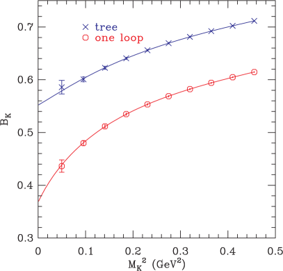
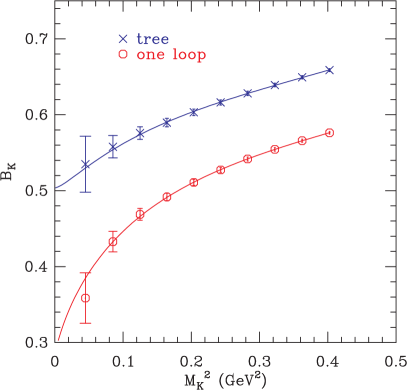
Figure 1: Tree-level and one-loop matched $B_{K}$ versus $M_{K}^{2}$ for degenerate valence quarks. Results are for the coarse (left) and fine (right) MILC lattices with $m_{l}/m_{s}=0.01/0.05$.

In Fig. 1, we show the results for $B_{K}$ on coarse ($a\approx 0.12\;$fm) and fine ($a\approx 0.09\;$fm) lattices before and after inclusion of the one-loop corrections. For clarity, we show only the points in which the valence quarks are degenerate. The roughly 20% reduction caused by the inclusion of one-loop contributions holds also for non-degenerate valence quarks. We also show the results of a four-parameter partial NNLO fit.

The size of the one-loop shift ($\approx 20\%$) is of the expected magnitude, given that $\alpha_{s}(1/a)$ is $\approx 0.33$ and $0.27$ on the coarse and fine lattices, respectively. It should be kept in mind that, however, that $B_{K}$ is scale dependent, and so the one-loop correction can be made larger or smaller by varying the scale chosen in the continuum operator. In other words, there is no precise way of defining the size of the correction.

A noteworthy feature of these results is that the curvature at small $M_{K}$ is larger after one-loop matching, This is even more pronounced in the results on the superfine lattices ($a\approx 0.06\;$fm), shown in Fig. 2. Indeed, one can see that the fit to the tree-level results has an upwards “hook” at very small $M_{K}$, which is the result of the fit requiring a significant contribution from the taste-violating operators which are present because of truncation (and discretization) errors. These contributions behave as $-\log M_{K}$ in the chiral limit, and are finite there because the kaon that appears has non-Goldstone taste and so its mass does not vanish in the chiral limit. We expect such contributions to be of leading order in SChPT for tree-level matching, but of NLO, and thus much smaller, for one-loop matching. This is consistent with our results. We stress that the curvature seen in the one-loop curves is not a surprise as the chiral logarithm has a fairly large coefficient.

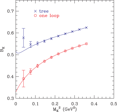
Figure 2: $B_{K}$ vs. $M_{K}^{2}$ for the MILC superfine lattice with $m_{l}/m_{s}=1/5$.

The subset of the data most relevant to extrapolating to the physical kaon is that in which the valence kaon is maximally non-degenerate. This effect of one-loop matching on this subset of the data is illustrated by Fig. 3, where we present the results of the SU(2) SChPT fits $B_{K}$ on the coarse MILC lattices. We show an example of the “X-fit” (the extrapolation in $M_{\pi}^{2}$ for fixed valence strange-quark mass) and the “Y-fit” (the extrapolation in the valence strange quark mass). These fits are explained in Ref. [2].

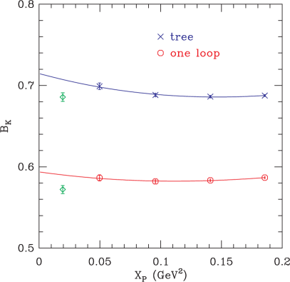
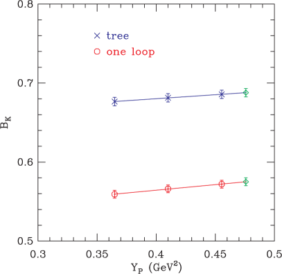
Figure 3: $B_{K}$ vs. $X_{P}$ (left: X-fit) and vs. $Y_{P}$ (right: Y-fit) on the MILC coarse lattices (right: Y-fit) with $m_{l}/m_{s}=1/5$. The [green] diamonds in the left plot show the result after extrapolation to the physical pion mass, $X_{P}=M_{\pi}^{2}$, and removal of lattice artefacts from the fit function. In the right panel the [green] diamonds show the result of an extrapolation to the physical valence strange quark mass.

3 RG Evolution

The fitting procedures described in Refs. [1, 2] result in values for $B_{K}(1/a)$ on the three lattice spacings, with taste-breaking discretization and truncation errors removed. In order to compare these values we next run them from $1/a$ to a common scale, which we take to be $2\;$GeV. Here, we use two-loop RG evolution

$$B_{K}^{\text{NDR}}(p) = \frac{[1-\frac{\alpha(q^{*})}{4\pi}Z]}{[1-\frac{\alpha(p)}{4\pi}Z]}\bigg{(}\frac{\alpha(p)}{\alpha(q^{*})}\bigg{)}^{d^{(0)}}B_{K}^{\text{NDR}}(q^{*})$$

$$Z = \frac{\gamma^{(1)}}{2\beta_{0}}-d^{(0)}\frac{\beta_{1}}{\beta_{0}}$$

$$d^{(0)} = \frac{\gamma^{(0)}}{2\beta_{0}}$$

where the anomalous dimension matrices $\gamma^{(i)}$, and the beta-function coefficients, $\beta_{i}$, are given, e.g., in Ref. [11].

After RG running, we have values of $B_{K}({\rm NDR},\mu=2\ {\rm GeV})$ from the three lattices spacings, which still contain discretization and truncation errors. We attempt to remove the former by a linear extrapolation in $a^{2}$, as described in Ref. [2]. As for the latter, we attempt to estimate these separately, as we now describe.

4 Estimate of Two-Loop Terms

Let $B_{K}^{(i)}$ be the value of $B_{K}$ obtained using parallel matching ($\mu=1/a$) at the $i$’th loop level, and after extrapolation to the physical valence and sea-quark masses. Then we can define $\Delta B_{K}^{(i)}$ as

$$\Delta B_{K}^{(i)}\equiv B_{K}^{(i-1)}-B_{K}^{(i)}\,.$$ (5)

so that $\Delta B_{K}^{(i)}$ represents the shift due to the $i$’th loop correction to $B_{K}$. We know $B_{K}^{(0)}$ and $B_{K}^{(1)}$ and so we can calculate $\Delta B_{K}^{(1)}$; the results are collected in Table 1 for the SU(3) fits, and Table 2 for the SU(2) fits. One estimate of $\Delta B_{K}^{(2)}$ is then

$$\Delta B_{K}^{(2)}\approx\Delta B_{K}^{(1)}\times\alpha_{s}(1/a)\,,$$ (6)

with results also given in the Tables.

We plot $\Delta B_{K}^{(2)}$ versus $\alpha_{s}(1/a)^{2}$ for the two analyses in Fig. 4. Linear fits yield intercepts consistent with zero. This is not surprising given that $\Delta B_{K}^{(1)}$ is obtained from a one-loop matching formula, eq. (1), in which the correction is proportional to $\alpha_{s}(1/a)$, and is then multiplied by $\alpha_{s}(1/a)$ again to obtain $\Delta B_{K}^{(2)}$. The vanishing of the intercept is is not, however, an automatic result because the one-loop matching is applied before fitting and extrapolating the data, and involves contributions from lattice operators having different dependence on the quark masses. This means that $\Delta B_{K}^{(1)}$ need not be exactly linear in $\alpha_{s}(1/a)$.

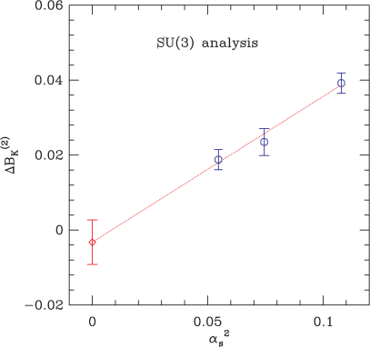
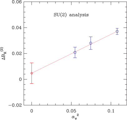
Figure 4: $\Delta B_{K}^{(2)}$ vs. $\alpha_{s}^{2}$ for the SU(3) analysis (left) and for the SU(2) analysis (right).

An alternative estimate is simply to use

$$\Delta B_{K}^{(2)^{\prime}}=B_{K}^{(0)}\times\alpha_{s}(1/a)^{2}\,,$$ (7)

i.e. the naive estimate of the two-loop contribution. This turns out to be somewhat larger than $\Delta B_{K}^{(2)}$, as shown in the Tables. It also varies more rapidly with the lattice spacing.

Since we extrapolate to the continuum limit assuming a linear dependence on $a^{2}$, the more slowly varying truncation error does not extrapolate to zero, although it will be somewhat reduced from the value at our smallest lattice spacing. To be conservative however, we take the value of the truncation error for the superfine lattices, and we use the larger of the two estimates, i.e. $\Delta B_{K}^{(2)^{\prime}}$. This gives the estimates that are included in the error budgets presented in Refs. [2, 3].

There are various ways in which one can firm up and reduce the truncation error. One is to work on a yet finer lattice, which might allow one to fit to a combination of $a^{2}$ and $\alpha^{2}$ errors, and will, in any case, reduce the size of the error. Another is to use two-loop matching. And, finally, one can remove all truncation errors, and replace them with statistical and some new systematic errors, by using non-perturbative renormalization. We are pursuing all three approaches.

$a$ (fm)	$B^{(0)}_{K}$	$B^{(1)}_{K}$	$\Delta B_{K}^{(1)}$	$\alpha_{s}(1/a)$	$\Delta B_{K}^{(2)}$	$\Delta B_{K}^{(2)^{\prime}}$
0.12	0.6898(59)	0.5704(58)	0.1194(83)	0.3285	0.039	0.074
0.09	0.6118(95)	0.5256(92)	0.0862(132)	0.2729	0.024	0.046
0.06	0.5963(83)	0.5158(80)	0.0805(115)	0.2337	0.019	0.033

Table 1: Results for tree-level and one-loop parallel-matched $B_{K}$ using the SU(3) SChPT analysis (fit N-BT7). For all lattice spacings we use the MILC lattices for which $m_{l}/m_{s}=1/5$. Also given are the one-loop shift, the value of $\alpha_{s}$, and estimates of the two-loop shift.

$a$ (fm)	$B^{(0)}_{K}$	$B^{(1)}_{K}$	$\Delta B_{K}^{(1)}$	$\alpha_{s}$	$\Delta B_{K}^{(2)}$	$\Delta B_{K}^{(2)^{\prime}}$
0.12	0.6879(53)	0.5751(49)	0.1128(72)	0.3285	0.037	0.074
0.09	0.6383(130)	0.5358(122)	0.1025(178)	0.2729	0.028	0.048
0.06	0.5829(128)	0.4937(119)	0.0892(175)	0.2337	0.021	0.032

Table 2: As for Table 1 except using the SU(2) SChPT analysis (4X3Y-NNLO fit).

5 Acknowledgments

C. Jung is supported by the US DOE under contract DE-AC02-98CH10886. The research of W. Lee is supported by the Creative Research Initiatives Program (3348-20090015) of the NRF grant funded by the Korean government (MEST). The work of S. Sharpe is supported in part by the US DOE grant no. DE-FG02-96ER40956. Computations were carried out in part on facilities of the USQCD Collaboration, which are funded by the Office of Science of the U.S. Department of Energy.

References

- [1] Taegil Bae, et al., PoS (LAT2009) 261.
- [2] Hyung-Jin Kim, et al., PoS (LAT2009) 262.
- [3] Boram Yoon, et al., PoS (LAT2009) 263.
- [4] T. Bae, et al., in preparation.
- [5] G. Kilcup, R. Gupta and S.R. Sharpe, Phys. Rev. D 57, 1654 (1998) [arXiv:hep-lat/9707006].
- [6] Yasumichi Aoki, PoS (LAT2009) 012.
- [7] A. Lytle, PoS (LAT2009) 202.
- [8] W. Lee and S.R. Sharpe, Phys. Rev. D 68, 054510 (2003) [arXiv:hep-lat/0306016].
- [9] Jongjeong Kim, Weonjong Lee and Stephen R. Sharpe, in preparation.
- [10] Ruth S. Van de Water, Stephen R. Sharpe, Phys. Rev. D73 (2006) 014003, [hep-lat/0507012].
- [11] Andrzej J. Buras, Matthias Jamin, and Peter Weisz, Nucl. Phys. B347 (1990) 491.