Time complexity and gate complexity

Abstract

We formulate and investigate the simplest version of time-optimal quantum computation theory (t-QCT), where the computation time is defined by the physical one and the Hamiltonian contains only one- and two-qubit interactions. This version of t-QCT is also considered as optimality by sub-Riemannian geodesic length. The work has two aims: one is to develop a t-QCT itself based on physically natural concept of time, and the other is to pursue the possibility of using t-QCT as a tool to estimate the complexity in conventional gate-optimal quantum computation theory (g-QCT). In particular, we investigate to what extent is true the statement: time complexity is polynomial in the number of qubits if and only if so is gate complexity. In the analysis, we relate t-QCT and optimal control theory (OCT) through fidelity-optimal computation theory (f-QCT); f-QCT is equivalent to t-QCT in the limit of unit optimal fidelity, while it is formally similar to OCT. We then develop an efficient numerical scheme for f-QCT by modifying Krotov’s method in OCT, which has monotonic convergence property. We implemented the scheme and obtained solutions of f-QCT and of t-QCT for the quantum Fourier transform and a unitary operator that does not have an apparent symmetry. The former has a polynomial gate complexity and the latter is expected to have exponential one which is based on the fact that a series of generic unitary operators has a exponential gate complexity. The time complexity for the former is found to be linear in the number of qubits, which is understood naturally by the existence of an upper bound. The time complexity for the latter is exponential in the number of qubits. Thus the both targets seem to be examples satisfyng the statement above. The typical characteristics of the optimal Hamiltonians are symmetry under time-reversal and constancy of one-qubit operation, which are mathematically shown to hold in fairly general situations.

I Introduction

Quantum computation is performed by physical processes obeying quantum mechanics. It became one of the most exciting field in physics and information theory after Shor shor discovered an algorithm to factorize integers which is exponentially faster than any known classical ones. In quantum computation theory (QCT), as in classical computation theory, the computation time is usually defined by the number of elementary steps or gates necessary to perform a computation, i.e., to realize a desired unitary operator. Minimum such number is called the gate complexity. We shall call this conventional QCT as gate-optimal QCT (g-QCT).

In this paper, we investigate time-optimal quantum computation theory (t-QCT) where the computation time is defined by physical time. There are two motivations for t-QCT. The first is to develop (an abstract) t-QCT itself which is a physical-time-based alternative to g-QCT. Since a quantum computation is a physical process, it is physically more natural to measure the time by the physical one. From this viewpoint, the computation time in g-QCT can be seen as information-theoretic time which is a more abstract or coarse-grained notion of time than the physical one. Time optimality is attracting growing attention in quantum optimal control theory (OCT) mainly in the context of physical applications such as control of an atom by an electromagnetic field and NMR quantum computation (khaneja ; schulte and references therein).

The second motivation, which we stress in the present work and state in detail in Sec. II.2, is that t-QCT may be a useful tool to analyze g-QCT. Finding the gate-optimal algorithm is a discrete and combinatorial problem, which makes construction of a general theory difficult. On the other hand, time-optimal algorithms are smooth curves in a certain space which obeys a differential equation paper1 ; paper2 ; paper3 , typically that for a sub-Riemannian geodesic montgomery on a manifold. This may allow a general theory and approximation methods. Moreover, roughly speaking, upper and lower bounds for gate complexity can be given in terms of optimal physical time nielsen1 ; nielsen2 . Thus t-QCT is useful in the investigation of g-QCT. One may become able to calculate gate complexity by calculating time complexity. We ask to what extent holds the statement that the time complexity is polynomial in the number of qubits if and only if so is the gate complexity.

We will therefore compare the time complexity and the gate complexity for some typical examples. We choose the quantum Fourier transform (QFT) as an example of the target unitary operator of which a fast algorithm in the sense of g-QCT (i.e. whose gate complexity is polynomial in the number of qubits) is known, while we choose a target unitary with no special symmetry because a generic series of target unitary operators is known not to have fast algorithms.

To achieve it, we will make use of an efficient numerical method for OCT, so-called Krotov’s method. We relate t-QCT to fidelity-optimal QCT (f-QCT), and develop a Krotov-like scheme for f-QCT by making use of the formal similarity of f-QCT and OCT. In the context of OCT, similar ideas of replacing time optimality to fidelity optimality have been used.

We will see that both the QFT and the asymmetric unitary operator satisfy the statement above. Furthermore, we will find some characteristic behaviour of the optimal Hamiltonian, namely, time-reversal symmetry and constancy of one-qubit Hamiltonian components.

In analyzing t-QCT, it is useful to combine numerical and mathematical approaches. We will show mathematically that the behavior which is found numerically is satisfied in fairly general situations. These arguments in turn support the soundness of our numerical calculation.

The organization of the paper is as follows. In Sec. II, we introduce t-QCT as a special case of quantum brachistochrone paper1 ; paper2 ; paper3 and explain our above-mentioned motivation more precisely. In Sec. III, we discuss the relation between t-QCT and f-QCT. In Sec. IV, we present a Krotov-like numerical method for f-QCT. We will show our numerical results and extract the properties of the solutions of f-QCT and of t-QCT in Sec. V. We will give a proof of time-reversal invariance and constancy of one-qubit components in Sec. VI. Sec. VII is for conlusion. In Appendix A we show the monotonicity of the numerical scheme of Sec. IV, and in Appendix B we give a proof of a theorem in Sec. VI.

We use the units $\hbar=1$.

II Time-optimal QCT

In this section, we introduce t-QCT, with some review of quantum brachistochrone, and present the motivation of the paper in more detail.

II.1 Definition

Let us define the simplest version of time-optimal QCT (t-QCT) as a special case of quantum brachistochrone for unitary operations paper2 , namely, the case in which the Hamiltonian $H(t)$ involves only one- and two-qubit interactions and is subject to a normalization constraint. Below is a summary of the formalism paper2 in this case.

Quantum brachistochrone for unitary operations is a framework to find the optimal Hamiltonian $H(t)\in\Gamma$ which realizes the desired unitary $U_{f}$ up to phase in the minimum time $T\geqslant 0$, where $\Gamma$ is the set of available Hamiltonians. Namely, one wants to find the minimum $T$ such that there is a unitary operator $U(t)$ satisfying the Schrödinger equation

$$i\dot{U}(t)=H(t)U(t),$$ (1)

and the initial and final conditions,

$$U(0) ={{\bf 1}},$$ (2)

$$U(T) =e^{-i\chi}U_{f},$$ (3)

where ${\bf 1}$ is the identity operator and $\chi$ is some real.

For t-QCT of the system of $n$ qubits, the set $\Gamma$ of available Hamiltonians consists of self-adjoint operators

$$H(t)=\sum_{a}h_{a}(t)\tau_{a}$$ (4)

with a normalization constraint

$$|h(t)|^{2}:=\sum_{a}(h_{a}(t))^{2}=N\omega^{2},$$ (5)

where $N:=2^{n}$ and the basis $\{\tau_{a}\}$ consists of $\sigma^{a}_{j}/\sqrt{N}$ and $\sigma^{ab}_{jk}/\sqrt{N}$. Here, $\sigma^{a_{1}\cdots a_{m}}_{j_{1}\cdots j_{m}}$ ($1\leqslant a_{1}<\cdots<a_{m}\leqslant n$ and $j_{l}=x,y,z$) denotes the direct product of the Pauli operator $\sigma_{j_{l}}$ on the $a_{l}$th qubit and identities on the others; for example, $\sigma^{13}_{xy}=\sigma_{x}\otimes 1\otimes\sigma_{y}\otimes 1\otimes\cdots\otimes 1$. The normalization condition 5 can be interpreted physically as finiteness of available energy in operations, while it is needed mathematically for the optimality problem to be well-posed paper1 . The $N$-dependence of 5 is for consistency under composition of systems paper3quantph . The parameter $\omega$ can be interpreted as defining a unit for $T$. The problem is a particular case of linear homogeneous constraints (paper2, , Sec. III).

This is the natural counterpart in t-QCT to the standard paradigm in g-QCT where one constructs a desired unitary by a sequence of one- and two-qubit operations. The parameter $\omega$ can be interpreted as defining a unit for $T$. The problem is a particular case of quantum brachistochrone for linear homogeneous constraints (paper2, , Sec. III).

In the form of variational principle, t-QCT is to minimize the action

$$S(U,h,V,\overline{\lambda})=\int_{0}^{T}dt\Bigl{[}L_{T}+L_{S}+\frac{\check{\lambda}(t)}{2}(|h(t)|^{2}-N\omega^{2})\Bigr{]},$$ (6)

where $L_{T}:=\sqrt{\frac{\operatorname{Tr}{\dot{U}^{\dagger}(1-P_{U})(\dot{U})}}{\operatorname{Tr}{(HU)^{\dagger}(1-P_{U})(HU)}}}$, $P_{U}(A):=\frac{1}{N}(\operatorname{Tr}AU^{\dagger})U$, $L_{S}:=2{\rm Re}\operatorname{Tr}V^{\dagger}\bigl{(}{i\dot{U}-HU}\bigr{)}$, an overdot denotes time derivative. The first term counts the time duration, where $L_{T}$ is unity when the Schrödinger equation 1 holds and is invariant under time reparametrization $t\mapsto f(t)$ fn-a . The second term $L_{S}$ guarantees that the Schrödinger equation 1 holds at all times where the unitary operator $V(t)$ is the Lagrange multipliers. The third term guarantees the normalization constraint 5 where the real function $\check{\lambda}(t)$ is Lagrange multiplier. We have adopted an action equivalent to but slightly different in form from that in Ref. paper2 for better connection with the arguments below.

We note that the phase of $U(t)$ does not matter in the present formulation of t-QCT. In fact, the action 15 is invariant under a time-dependent phase change of $U(t)$ which can be considered as a gauge transformation paper2 . Therefore the theory is defined on $\operatorname{\rm U}(N)/\operatorname{\rm U}(1)$, and one can also think of it as a theory on $\operatorname{\rm SU}(N)$ (by “gauge fixing”).

The Euler-Lagrange equations are paper2 the Schrödinger equation 1 for $U(t)$, the normalization constraint 5, the Schrödinger equation for $V(t)$,

$$i\dot{V}(t) =H(t)V(t),$$ (7)

and the equation determining $H(t)$,

$$\lambda(t)h_{a}(t) =\operatorname{Tr}\tau_{a}F(t),\quad F(t):=U(t)V^{\dagger}(t)+V(t)U^{\dagger}(t),$$ (8)

where $\lambda(t):=\check{\lambda}(t)-\frac{1}{N\omega^{2}}$. One must solve these equations with the initial and final conditions 2 and 3.

Let us recall some general features of the system. First, $F$ satisfies the simple evolution equation

$$i\dot{F}(t)=[H(t),F(t)],$$ (9)

which follows from 1, 7 and 8. Second, the expression for $\lambda(t)$ is

$$\lambda(t)=\frac{1}{\omega}\sqrt{\frac{1}{N}\sum_{a}{\left(\operatorname{Tr}\tau_{a}F(t)\right)}^{2}},$$ (10)

which follows from 5 and 8. Third, this variable $\lambda(t)$ is constant in time fn-b .

In the special case when $U_{f}$ is a one- or two-qubit operation in $\operatorname{\rm U}(N)$, the solution of t-QCT is given by a Riemannian geodesic $U(t)=e^{-iHt}$ on $\operatorname{\rm U}(N)/\operatorname{\rm U}(1)$, where $H$ is constant paper1 ; paper2 . The time $T(U_{f})$ is proportional to the arc length and depends solely on the eigenvalues $e^{i\theta_{j}}$ of the relevant $\operatorname{\rm SU}(4)$ part of $U_{f}$ as

$$T(U_{f})=\frac{1}{2\omega}\sqrt{\min_{\chi,m_{j}}\sum_{j=1}^{4}(\theta_{j}+2\pi m_{j}-\chi)^{2}},$$ (11)

where $\chi$ is a real and $m_{j}$ are integers. For example, the time is given by $T(U_{\scriptsize\mbox{CNOT}})=T(S)=\frac{\sqrt{3}\pi}{4\omega}$ for the controlled NOT gate $U_{\scriptsize\mbox{CNOT}}$ and SWAP gate $S$ whose eigenvalues are $(1,1,1,-1)$, and $T_{2,\scriptsize\mbox{max}}=\frac{\sqrt{5}\pi}{4\omega}$ for the hardest two-qubit operation whose eigenvalues are $(1,i,-1,-i)$. These can be used for the unit of $T(U_{f})$ in comparing $T(U_{f})$ with $G(U_{f})$.

II.2 t-QCT, g-QCT and our motivation

There are some rigorous relations between the gate complexity and time complexity. Very roughly speaking, one can give upper and lower bounds for gate complexity through the time complexity.

Before introducing the relations, recall that in the simple cases, the time complexity $T(U)$ can also be interpreted as the arc length $L(U)$ of the sub-Riemannian geodesic connecting ${\bf 1}$ and $U_{f}$, up to overall multiplicative constant. The simplest version of t-QCT presented in Sec. II.1 falls into this category, so that $\frac{T(U)}{T_{2,\scriptsize\mbox{max}}}$ appearing below in this paper can also be considered as $\frac{L(U)}{L_{2,\scriptsize\mbox{max}}}$ where $L_{2,\scriptsize\mbox{max}}$ is the sub-Riemannian geodesic distance between ${\bf 1}$ and the furthest two-qubit operation.

The precise relations are given (nielsen2, , esp. Eq. (15)) by

$$\frac{T(U)}{T_{2,\scriptsize\mbox{max}}}\leqslant G(U),\quad G(U,\epsilon)\leqslant\frac{AT(U)^{3}n^{6}}{\epsilon^{2}},$$ (12)

where $T(U)$ is the time complexity to realize the unitary $U$, and $G(U,\epsilon)$ is the gate complexity to realize a unitary within the distance $\epsilon$ from $U$ (measured in the operator norm), $T_{2,\scriptsize\mbox{max}}$ is the constant defined in the previous section, and $A$ is some constant. Note that we always have $G(U,\epsilon)\leqslant G(U)$.

Let us explain the first inequality of 12 which is simple. For a one- or two-qubit gate $U$, we have $\frac{T(U)}{T_{2,\scriptsize\mbox{max}}}\leqslant 1=G(U)$ by the definition of $T_{2,\scriptsize\mbox{max}}$. Then, for a general $U$, letting $U=U_{m}\cdots U_{1}$ be the gate-optimal decomposition, we have $\frac{1}{T_{2,\scriptsize\mbox{max}}}\sum_{j=1}^{m}T(U_{j})\leqslant G(U)$. However, the sum in the LHS, the time cost of this decomposition, must be greater than or equal to the time complexity $T(U)$ of $U$. Thus the first inequality of 12 holds.

The relation 12 is suggestive, and one might expect that

$$G(U)\approx T(U),$$ (13)

by which we mean that $G(U)$ and $T(U)$ are bounded by some polynomial of each other and $n$. However, it is argued that this cannot be true in general nielsen2 . Then, one may want to ask to what extent 13 is true in general, since 12 is derived by a completely general argument. In particular, we think that it is interesting to ask what are the classes of unitary operators $U$ which satisfy

1. $T(U)\approx G(U)$, i.e., $T(U)$ and $G(U)$ are bounded by a polynomial of each other and $n$,

2. $T(U)\sim G(U)$, i.e., $T(U)$ is polynomial in $n$ if and only if so is $G(U)$.

The second class contains the first class. Note that the first and second conditions above are equiavlent to $G(U)\approx G(U,\epsilon)$ and $G(U)\sim G(U,\epsilon)$, respectively, by 12. The questions above are not easy, but we want to develop a basis here which will help answering these questions in the future.

t-QCT itself is a good framework to analyze these questions theoretically. However, a drawback is that it is extremely hard in practice to derive exact solutions when $n$ is large. One way is to appeal to numerical calculations, but it is also difficult because one encounters a two-point boundary value problem in dimensions rapidly increasing with $n$. In Ref. schulte , time-optimal solutions were obtained up to seven qubits for the like of Hamiltonians appearing in NMR quantum computers. That problem involves $2n$ ($\lesssim 20$ for $n\lesssim 10$) functions for the boundary value problem. Our t-QCT has $9n(n-1)/2+3n$ functions, where the number easily becomes several hundred. To minimize the numerical difficulty, we introduce a problem bridging t-QCT and optimal control theory (OCT), and make use of an efficient numerical scheme for the latter.

III Fidelity-optimal QCT

In this section, we relate t-QCT to f-QCT and prepare for introducing the numerical method in the next section. In the context of OCT, similar ideas of relating time optimality and fidelity optimality are used (e.g. schulte ).

III.1 Definition

Let us define fidelity-optimal QCT (f-QCT) as a framework to solve the following problem: given a target unitary operator $U_{f}$ and time interval $T$, find the Hamiltonian $H(t)\in\Gamma$ as a function of time which maximizes the fidelity ${\cal F}(U(T),U_{f})$. Here we use the trace fidelity

$${\cal F}(U(T),U_{f}):=\frac{1}{N}|\operatorname{Tr}U^{\dagger}U_{f}|$$ (14)

because we want $U(T)$ to be close to $U_{f}$ only up to phase. The problem is to minimize the action

$$S(U,h,V,\lambda) =-N{\cal F}(U(T),U_{f})^{2}$$

$$+\int_{0}^{T}dt\Bigl{[}L_{S}+\frac{\lambda(t)}{2}(|h(t)|^{2}-N\omega^{2})\Bigr{]}.$$ (15)

The first term is the squared fidelity of the final unitary $U(T)$ with respect to the target $U_{f}$. The second and third terms guarantee the Schrödinger equation 1 and the normalization constraint 5, respectively, as in the case of t-QCT. The action 15 is invariant under the (time-dependent) change of the phase of $U(t)$ so that the theory is defined on $\operatorname{\rm U}(N)/\operatorname{\rm U}(1)$.

The Euler-Lagrange equations yield 1, 7, 8, and

$$V(T) =\frac{i}{N}U_{f}{\operatorname{Tr}U_{f}^{\dagger}U(T)}.$$ (16)

Therefore all the equations 1–10 hold except that 3 is replaced by 16. As in the case of t-QCT, $\lambda(t)$ is constant in time.

The solution gives the maximal fidelity ${\cal F}(U(T),U_{f})$ for given $T$. f-QCT is important on its own when one discusses the tradeoff between speed and error of computation. here we use f-QCT to bridge t-QCT and OCT.

III.2 Relation between solutions to f-QCT and t-QCT

The solution of t-QCT can be obtained from that of f-QCT in the limit ${\cal F}\to 1$.

First, f-QCT is equivalent to the problem of minimizing the physical time to achieve given fidelity. Suppose the solution $U_{0}(t)$ of f-QCT for given time $T_{0}$, with optimal fidelity ${\cal F}(U(T_{0}),U_{f})=f$, was not the solution of the above new problem. There would be $\check{U}(t)$ achieving the same fidelity in some $T<T_{0}$. Then one could construct $U(t)$ with ${\cal F}(U(T_{0}),U_{f})>f$ by defining $U(t)=\check{U}(t)$ for $0\leqslant t\leqslant T$ and appropriately in $T<t\leqslant T_{0}$. This would contradict to the fact that $U_{0}(t)$ is a solution of f-QCT. Thus $U_{0}(t)$ is the solution of the above problem. The converse is shown similarly.

Second, the above new problem with fixed fidelity $f$ yields t-QCT when $f\to 1$. Therefore the solution of f-QCT gives that of t-QCT in the limit ${\cal F}\to 1$.

III.3 Formal similarity of f-QCT and OCT

Let us see the formal similarity between f-QCT and OCT.

Our action 15 defines an exact fidelity optimality problem with constraints. If we replace $\lambda(t)$ with a given constant or a given function, the term $\frac{\lambda(t)|h(t)|^{2}}{2}$ in the integral can be interpreted as a penalty term while the constant term $-\frac{\lambda(t)N\omega^{2}}{2}$ may be dropped. Then the problem is to minimize a combination of the fidelity and penalty terms with their weights specified by $\lambda(t)$, which is a typical problem in OCT. This is the formal relation between f-QCT and OCT.

IV A Krotov-like scheme

In this section, we shall define an efficient numerical scheme for f-QCT by modifying Krotov’s method tannor in OCT, making use of the similarity between f-QCT and OCT in Sec. III.3.

In what follows, the functions $\overline{h}_{a}(t)$ and $\overline{\lambda}(t)$, respectively, are $h_{a}(t)$ and $\lambda(t)$ calculated in the middle of an iteration cycle of the scheme, and Eqs. $\overline{\ref{eq-normalization}}$, $\overline{\ref{eq-schv}}$ and $\overline{\ref{eq-lambda}}$, respectively, denote Eqs. 5, 7 and 8 with $h_{a}(t)$ (including that in $H(t)$) and $\lambda(t)$ being replaced by $\overline{h}_{a}(t)$ and $\overline{\lambda}(t)$. The scheme is as follows.

(i) Prepare a seed Hamiltonian components $h_{a}(t)$, $0\leqslant t\leqslant T$.

(ii) Set $U(0)=1$ and evolve $U(t)$ from $t=0$ to $t=T$ by 1 with the Hamiltonian $H(t)=\sum_{a}h_{a}(t)\tau_{a}$.

(iii) Set $V(T)$ by 16 and evolve $(V(t),\overline{h}_{a}(t),\overline{\lambda}(t))$ backward in time from $t=T$ to $t=0$ by Eqs. $\overline{\ref{eq-schv}}$, $\overline{\ref{eq-lambda}}$ and $\overline{\ref{eq-lambda-2}}$, while $U(t)$ is treated as a given function and is not updated.

(iv) Set $U(0)=1$ and evolve $(U(t),h(t),\lambda(t))$ forward in time from $t=0$ to $t=T$ by Eqs. 1, 8 and 10, while $V(t)$ is treated as a given function.

(v) Repeat steps (iii) and (iv) until the variables converge; the final $h_{a}(t)$ defines the optimal Hamiltonian and the final ${\cal F}(U(T),U_{f})$ gives the maximal achievable fidelity in $T$.

Note that the multiplier $\lambda(t)$ converges to an unknown constant only after the convergence, which is in contrast to original Krotov’s scheme where $\lambda$ is a given constant parameter of the problem. The constancy of $\lambda(t)$ can be used for a convergence check of the present scheme. The present scheme is also different from Krotov’s method for the case of a fixed reference energy (see, e.g. kosloff2 ). In the former, the variable $\lambda(t)$ is a Lagrange multiplier and the normalization 5 must be satisfied at all times, and $\lambda(t)$ is updated in the scheme. In the latter, $\lambda(t)$ is a given function which determines the amount of penalty imposed on the error in 5, and $\lambda(t)$ is not updated in the scheme. See also discussions in Sec. III.2.

An important property of our Krotov-like scheme is monotonicity, which is necessary for the scheme to be useful. We give the proof in Appendix A.

V Results

We implemented the numerical scheme presented in Sec. IV and performed calculations for f-QCT. We chose two examples for the target unitary operator $U_{f}$.

The first is the quantum Fourier transform (QFT) $U^{(n)}_{\rm QFT}$, defined by

$$U^{(n)}_{\rm QFT}|{x}\rangle=\frac{1}{\sqrt{N}}\sum_{k=0}^{k=N-1}e^{2\pi ikx/N}|{k}\rangle,\quad x=0,1,...,N-1,$$ (17)

which has the gate complexity $G(U_{f})$ polynomial in $n$. In fact, a simple efficient algorithm (e.g. chuangnielsen ) is given by

$$U^{(n)}_{\rm QFT} =S_{n_{2},n-n_{2}}\cdots S_{1n}U_{1}\cdots U_{n},$$

$$U_{j} :=R_{j,n-j+1,n}\cdots R_{2,n-j+1,n-j+2}W_{n-j+1},$$ (18)

where $W_{j}$ is the Walsch-Hadamard gate $W:=\frac{1}{\sqrt{2}}\begin{bmatrix}1&1\\ 1&-1\end{bmatrix}$ applied on the $j$th qubit, $R_{j,km}$ is the $2\pi/2^{j}$-phase shift gate $R_{j}:=\begin{bmatrix}1&0\\ 0&e^{2\pi i/2^{j}}\end{bmatrix}$ on the $k$th qubit controlled by the $m$th qubit, $S_{jk}$ is the SWAP gate $S$ on the $j$th and $k$th qubits, and $n_{2}:={\lfloor n/2\rfloor}$ (integer part of $n/2$). The number of gates of this construction is $n(n+1)/2+{\lfloor n/2\rfloor}$ so that $G(U^{(n)}_{\rm QFT})\leqslant n(n+1)/2+{\lfloor n/2\rfloor}\approx n^{2}$.

The second example of the target $U_{f}$ is chosen so that we can expect that $U_{f}$ has the gate complexity $G(U_{f})$ exponential in $n$. To do so, we pick a $U_{f}$ which does not have any apparent symmetry because a generic unitary operator $U_{f}$ has the gate complexity $G(U_{f})\approx 4^{n}$ and a unitary operator $U_{f}$ with a generic image of a fixed state vector, $U_{f}|{0}\rangle$, has the gate complexity $G(U_{f})\approx 2^{n}$ BulOLeBre05PRL . Our concrete choice is $U^{(n)}_{\scriptsize\rm asym}$ which is, in the matrix form,

$$U^{(n)}_{\scriptsize\rm asym}{}=\begin{bmatrix}\gamma_{0}\alpha_{0}&\gamma_{1}\alpha_{0}&\gamma_{2}\alpha_{0}&\cdots&\cdots&\gamma_{n-1}\alpha_{0}\\ \gamma_{0}\alpha_{1}&\gamma_{1}\beta_{1}&\gamma_{2}\alpha_{1}&\cdots&\cdots&\gamma_{n-1}\alpha_{1}\\ \vdots&0&\gamma_{2}\beta_{2}&\cdots&\cdots&\gamma_{n-1}\alpha_{2}\\ \vdots&\vdots&0&\ddots&&\vdots\\ \vdots&\vdots&\vdots&&\ddots&\vdots\\ \gamma_{0}\alpha_{n-1}&0&0&\cdots&\cdots&\gamma_{n-1}\beta_{n-1}\\ \end{bmatrix},$$ (19)

where $\alpha_{k}:=(k+1)^{1/3}e^{i\sqrt{k}}$, and $\beta_{j}\in{\mathbb{C}}$ and $\gamma_{j}>0$ are determined by orthogonalization and normalization, respectively, of the columns. The state vector $U^{(n)}_{\scriptsize\rm asym}|{0}\rangle$ is given by the first column of the right hand side of 19 which does not have apparent symmetry. One can therefore expect that the gate complexity is exponential in $n$, $G(U^{(n)}_{\scriptsize\rm asym})\mathrel{\mathchoice{\lower 2.58334pt\vbox{\halign{$\m@th\displaystyle\hfil#\hfil$\cr>\crcr\sim\crcr}}}{\lower 2.58334pt\vbox{\halign{$\m@th\textstyle\hfil#\hfil$\cr>\crcr\sim\crcr}}}{\lower 2.58334pt\vbox{\halign{$\m@th\scriptstyle\hfil#\hfil$\cr>\crcr\sim\crcr}}}{\lower 2.58334pt\vbox{\halign{$\m@th\scriptscriptstyle\hfil#\hfil$\cr>\crcr\sim\crcr}}}}2^{n}$.

For each given time $T$, the convergence of the scheme is checked by the convergence of the fidelity, and the constancy of $\lambda(t)$ explained in Sec. IV.

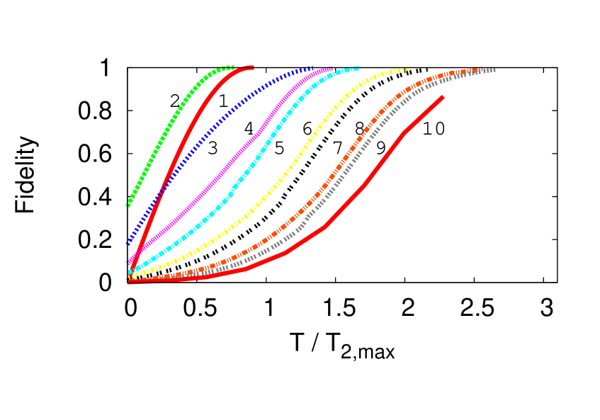
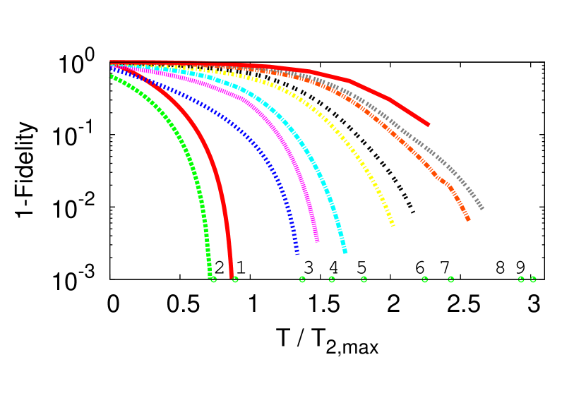
Figure 1: (Color online) (Upper) Optimal achievable fidelity in given physical time for the $n$-qubit QFT in f-QCT. The numbers beside the curves denote $n$. The $n=10$ result is preliminary. One can see property (a) in Sec. V.1. (Lower) The same graph with the vertical axis being $1-{\cal F}$ in logarithmic scale. The points and the numbers on the lower axis indicate the time complexity $T(U_{f})$ estimated by the fidelity$\to 1$ limit for each $n$.

V.1 Fidelity-time relation

Let us show the fidelity-time relation, namely, the maximal achievable fidelity ${\cal F}(U(T),U_{f})$ in time $T$. For simplicity, we only show the case of the QFT (Fig. 1).

Though our scheme in Sec. IV is monotonic, there is a possibility of the calculation is trapped by a local minimum of the action $S$. We did the following two things in order to find the global maximum ${\cal F}$. One is simply preparing many random seeds $h_{a}(t)$ for each $T$. Another is making use of the continuity of the solutions. Namely, we prepared many random seeds $h_{a}(t)$ for some fixed $T$. Then we used the solution for $T$ as the seed for a nearby $T$, and find continuous branches of locally optimal solutions. This “output recycling” turned out to be often more powerful than merely increasing the number of random seeds for every $T$. We observed crossovers of those branches. Only the branches of the largest ${\cal F}$ contribute to the curves in Fig. 1.

We observe the following, which may be characteristic of the QFT.

(a) The odd and even qubits seem to make a pair (4-5, 6-7, and 8-9) for $n\geqslant 4$.

In other words, the time-optimal solutions seems to split into the series of odd $n$ and that of even $n$, which may be useful in the future mathematical analysis of the time-optimal solutions of the QFT.

V.2 The limit ${\cal F}\to 1$

We estimate $T(U)$ from the limit ${\cal F}\to 1$ of the solutions to f-QCT in Sec. V.1.

In the limit, we have two sources of error. One is a natural numerical error which makes the fidelity ${\cal F}(U(T),U_{f})$ saturate below unity. Another is that if $T$ is larger or very close to the time complexity $T(U_{f})$, the solution of f-QCT for the physical time $T$ begin to “take a roundabout route” before reaching $U(T)$.

With this behaviour in mind, we estimate the time complexity by a nonlinear fitting of the fidelity-time curve around ${\cal F}(U(T),U_{f})\mathrel{\mathchoice{\lower 2.58334pt\vbox{\halign{$\m@th\displaystyle\hfil#\hfil$\cr>\crcr\sim\crcr}}}{\lower 2.58334pt\vbox{\halign{$\m@th\textstyle\hfil#\hfil$\cr>\crcr\sim\crcr}}}{\lower 2.58334pt\vbox{\halign{$\m@th\scriptstyle\hfil#\hfil$\cr>\crcr\sim\crcr}}}{\lower 2.58334pt\vbox{\halign{$\m@th\scriptscriptstyle\hfil#\hfil$\cr>\crcr\sim\crcr}}}}0.99$. Fig. 2 shows an example of the estimation, in the case of the $n=5$ QFT. We fit $y:=1-{\cal F}(U(T),U_{f})$ by $y=a(b-x)^{c}$, where $x:=T/T_{2,\scriptsize\mbox{max}}$. The estimation is given by $T(U_{f})/T_{2,\scriptsize\mbox{max}}\simeq b$. The error in the time complexity $T(U)/T_{2,\scriptsize\mbox{max}}$ is about $0.1$ in the case of QFT, and it is about $0.1$ or $0.2$ in the case of asymmetric unitary operator. This does not change the conclusion of the subsequent sections.

V.3 Time complexity as function of $n$

Let us discuss the behaviour of the time complexity as a function of number of qubits, $n$.

Fig. 3 shows the time complexity $T(U^{(n)}_{\rm QFT})$ in t-QCT as a function of $n$, where $T(U^{(n)}_{\rm QFT})$ is obtained by the value of $T$ on each curve in Fig. 1 in the limit ${\cal F}\to 1$. For $n=1$ and $n=2$, one has the exact values $\frac{T(U^{(1)}_{\rm QFT})}{T_{2,\scriptsize\mbox{max}}}=\frac{\pi}{2}/\frac{\sqrt{5}\pi}{4}=\frac{2}{\sqrt{5}}\approx 0.8944$ and $\frac{T(U^{(2)}_{\rm QFT})}{T_{2,\scriptsize\mbox{max}}}=\frac{\sqrt{11}\pi}{8}/\frac{\sqrt{5}\pi}{4}={\frac{\sqrt{1}1}{2\sqrt{5}}}\approx 0.7416$, calculated from 11, with which our numerical results agree well.

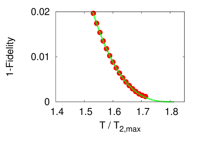
Figure 2: (Color online) Estimation of $T(U_{f})$ from the limit ${\cal F}\to 1$. In the $n=5$ QFT example, $y:=1-{\cal F}(U(T),U_{f})$ is fitted by $y=0.735(1.81-x)^{2.84}$, where $x:=T/T_{2,\scriptsize\mbox{max}}$, giving an estimate $T(U_{f})/T_{2,\scriptsize\mbox{max}}\simeq 1.81$. We used the data $0.002\leqslant y\leqslant 0.01$.

We observe the following property from Fig. 3.

(b) The optimal time $T(U^{(n)}_{\rm QFT})$ is linear in the number of qubits, $n$.

The line in Fig. 3 is the result of a linear fitting, which is $T(U_{f})/T_{2,\scriptsize\mbox{max}}=0.32n+0.27$. We used the data $n\geqslant 2$ in the fitting because the behaviour of $n\leqslant 2$ and that of $n\geqslant 2$ should differ due to the nature of $\Gamma$ allowing only interactions involving two qubits or less.

Property (b) is in good contrast to the number of gates, $O(n^{2})$, of the known efficient algorithm 18 for the $n$-qubit QFT. However, it can be understood naturally. Since $\frac{T(W)}{T_{2,\scriptsize\mbox{max}}}=\frac{2}{\sqrt{5}}$, $\frac{T(S)}{T_{2,\scriptsize\mbox{max}}}=\sqrt{\frac{3}{5}}$ and $\frac{T(R_{j,km})}{T_{2,\scriptsize\mbox{max}}}=\frac{1}{2^{j-1}}\sqrt{\frac{3}{5}}$ from 11, we have the physical time cost $T^{\prime}{}^{(n)}$ of the construction 18 is fn-c

$$\frac{T^{\prime}{}^{(n)}}{T_{2,\scriptsize\mbox{max}}}$$

$$\textstyle= \frac{1}{T_{2,\scriptsize\mbox{max}}}{\left[nT(W)+\sum_{j=2}^{n}(n-j+1)T(R_{j,km})+\left\lfloor\frac{n}{2}\right\rfloor T(S)\right]}$$

$$= \frac{2n}{\sqrt{5}}+\sqrt{\frac{3}{5}}\sum_{j=1}^{n-1}\frac{n-j}{2^{j}}+{\sqrt{\frac{3}{5}}}{\left\lfloor\frac{n}{2}\right\rfloor}$$

$$= \frac{2n}{\sqrt{5}}+\sqrt{\frac{3}{5}}{\left(n-2+\frac{1}{2^{n-1}}+\left\lfloor\frac{n}{2}\right\rfloor\right)},$$ (20)

which is bounded (from above and below) by a linear function of $n$. The time complexity $T(U^{(n)}_{\rm QFT})$ is several times smaller than $T^{\prime}{}^{(n)}$ (except for $n=1$ when they coincide). The significance of $T^{\prime}{}^{(n)}$ is that it is a rigorous upper bound for the time complesity, $T(U^{(n)}_{\rm QFT})\leqslant T^{\prime}{}^{(n)}$, which implies that $T(U^{(n)}_{\rm QFT})$ is at most linear in $n$. This strongly supports property (b) and the correctness of the numerical calculation.

Fig. 4 shows the time complexity $T(U_{f})$ as a function of $n$ for the case of the asymmetric target $U_{\scriptsize\rm asym}^{(n)}$.

We observe that

(b^′) The optimal time $T(U^{(n)}_{\scriptsize\rm asym})$ is exponential in the number of qubits, $n$.

As in the case of QFT, we used the data $n\geqslant 2$ to fit by a function. The time complexity $T(U_{\scriptsize\rm asym}^{(n)})$ is well fitted by an exponential function as $T(U_{\scriptsize\rm asym}^{(n)})/T_{2,\scriptsize\mbox{max}}=0.20\times 2^{0.82n}$. It is suggested from the numerical result that $U_{\scriptsize\rm asym}^{(n)}$ is in the class $T(U)\sim G(U)$.

To conclude, it is suggested that both the QFT and the asymmetric unitary are in the class $T(U)\sim G(U)$, which is polynomial in $n$ for the former and exponential in $n$ for the latter. [Note that in the polynomial case, $T(U)\sim G(U)$ implies $T(U)\approx G(U)$].

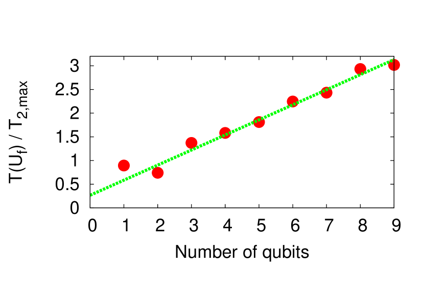
Figure 3: (Color online) Optimal time $T(U_{f})$ for realization of the QFT as a function of the number of qubits, $n$, with a linear least squares fitting for $n\geqslant 2$: $T(U_{f})/T_{2,\scriptsize\mbox{max}}=0.32n+0.27$.

V.4 Behavior of the time-optimal Hamitonian

Let us analyze the behavior of the optimal Hamiltonian $H(t)$ in t-QCT.

We shall say that an element of $\operatorname{\mathfrak{s}\mathfrak{u}}(N)$ is symmetric (or antisymmetric) if it is so in the standard matrix representation. In particular, $\tau_{a}$ is symmetric (antisymmetric) if it contains even (odd) number of $\sigma_{y}$; for example, $\sigma^{12}_{yy}/\sqrt{N}$ is symmetric and $\sigma^{12}_{xy}/\sqrt{N}$ is antisymmetric.

Fig. 5 is the behavior of the Hamiltonian $H(t)$ for the 4-qubit QFT with ${\cal F}\simeq 1$, which can be considered as the solution of t-QCT. The components $h_{a}$ are categorized into the four according to: whether $\tau_{a}$ is one- or two-qubit interaction, and whether $\tau_{a}$ is symmetric or antisymmetric.

The results suggest the following.

(c) The components for symmetric (antisymmetric) $\tau_{a}$ is symmetric (antisymmetric) under time-reversal $t\mapsto T-t$, and

(d) one-qubit interaction components are constant. Note that (c) and (d) imply that one-qubit antisymmetric components vanish.

The same properties are safisfied by the $n=5$ QFT. For the $n=3$ QFT, (c) does not hold but (d) does.

For the asymmetric target $U_{\scriptsize\rm asym}^{(n)}$, we do not observe property (c), the time reversal invariance. However, we do obverve property (d), constancy of one-qubit components, also in these cases. Fig. 6 shows the $n=3$ example of the behavior of the optimal Hamitonian.

These properties will be discussed from a theoretical point of view in Sec. VI.

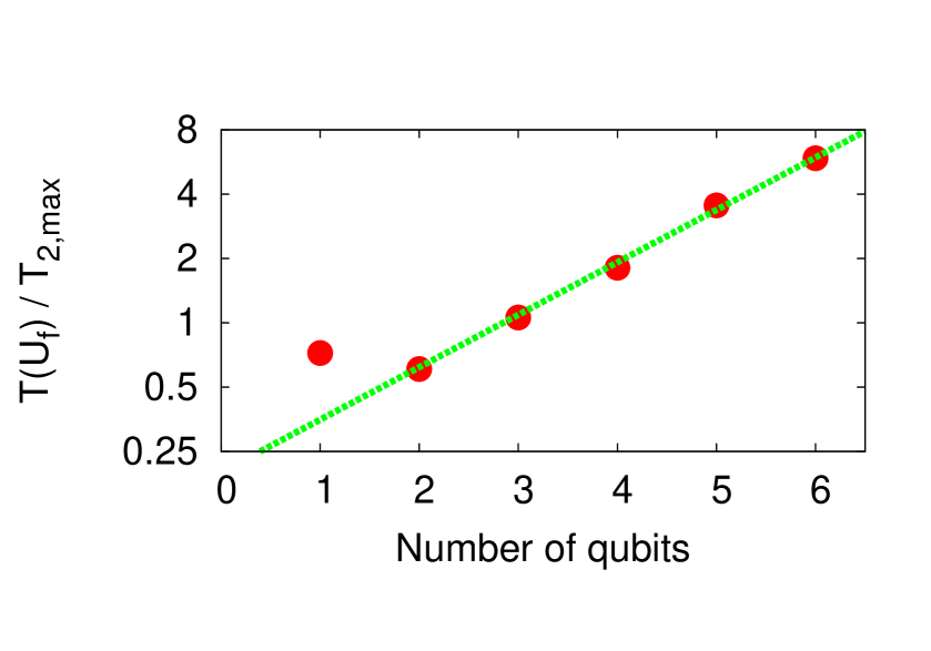
Figure 4: (Color online) Optimal time $T$ for realization of the asymmetric unitary $U_{\scriptsize\rm asym}^{(n)}$ as a function of the number of qubits, $n$, with a linear least squares fitting for $n\geqslant 2$: $T(U_{f})/T_{2,\scriptsize\mbox{max}}=0.20\times 2^{0.82n}$. Note that, in contrast to Fig 3, the vertical axis is in logarithmic scale.

VI Mathematical justification of the behaviour of the time-optimal Hamiltonian

The temporal behaviour of the optimal Hamiltonian in t-QCT found in Sec. V, property (c) for some of the QFT and property (d) for the QFT and the asymmetric unitary, are not peculiar to the case of those target unitary operators. They in fact can be proven under a fairly general condition. These results also serve as evidences of reliability of the numerical calculation.

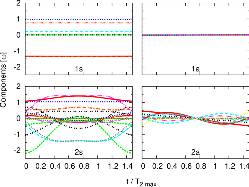
Figure 5: (Color online) Behavior of the optimal Hamiltonian for the 4-qubit QFT with $T/T_{2,\scriptsize\mbox{max}}=1.48$, ${\cal F}=.9967$. Shown are the components with respect to the generators which are (1s) one-qubit symmetric, (1a) one-qubit antisymmetric, (2s) two-qubit symmetric, and (2a) two-qubit antisymmetric, in the sense of Sec. V.3. The solution is time-reversal invariant. The one-qubit components are constant in time.

VI.1 Time reversal invariance

Let us show (c), the time-reversal symmetry found in some of the time-optimal solutions in Sec. V.

Let us define the time reversal $({U}_{\rm rev}(t),{H}_{\rm rev}(t),{V}_{\rm rev}(t),{\lambda}_{\rm rev}(t))$ of the set of variables, $(U(t),H(t),V(t),\lambda(t))$, by

$${U}_{\rm rev}(t) :=U^{*}(T-t)U^{T}(T),$$

$${H}_{\rm rev}(t) :=H^{*}(T-t)={\textstyle\sum_{a}}h_{a}(T-t)\tau_{a}^{*},$$

$${V}_{\rm rev}(t) :=V^{*}(T-t)U^{T}(T),$$

$${\lambda}_{\rm rev}(t) :=\lambda(T-t),$$ (21)

where the superscript asterisk denotes the complex conjugate and the superscript $T$ denotes the transpose. We have the following, whose proof is given in Appendix B.

Theorem 1.

Let the target $U_{f}$ be symmetric up to phase. If $(U(t),H(t),V(t),\lambda(t))$ is a solution of t-QCT for $U_{f}$ with optimal time $T$, so is $({U}_{\rm rev}(t),{H}_{\rm rev}(t),{V}_{\rm rev}(t),{\lambda}_{\rm rev}(t))$. In particular, if the solution is unique, it is invariant under time-reversal, $(U(t),H(t),V(t),\lambda(t))=({U}_{\rm rev}(t),{H}_{\rm rev}(t),{V}_{\rm rev}(t),{\lambda}_{\rm rev}(t))$.

The QFT is a symmetric target. The theorem justifies the observed symmetry property (c) of the QFT for $n\neq 3$. Convergence of ramdomly chosen initial Hamiltonians to a single time-symmetric solution suggests that the optimal solution is unique in those cases. The 3-qubit case did not show the symmetry, and consistently we observed many optimal solutions $H(t)$.

The asymmetric target unitary is not a symmetric operator and the numerical solutions did not show time-reversal invariance.

We remark that Theorem 1 holds not only in the present version of t-QCT but also in any quantum brachistochrone with $\Gamma^{*}=\Gamma$.

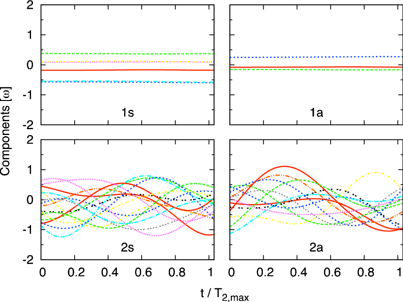
Figure 6: (Color online) Behavior of the optimal Hamiltonian for the 3-qubit asymmetric unitary $U^{(n)}_{\scriptsize\rm asym}$ with $T/T_{2,\scriptsize\mbox{max}}=1.03$, ${\cal F}=.9997$. Shown are the components with respect to the generators which are (1s) one-qubit symmetric, (1a) one-qubit antisymmetric, (2s) two-qubit symmetric, and (2a) two-qubit antisymmetric, in the sense of Sec. V.3. The solution is not time-reversal invariant. The one-qubit components are constant in time.

VI.2 Constancy of one-qubit components

Let us prove (d), which turns out to hold in general.

Theorem 2.

The one-qubit part of the Hamiltonian for any solution of t-QCT is constant in time.

Proof.

Let ${{\mathfrak{g}}}_{j}$ be the space of $j$-qubit operations. They satisfy the following commutation relations (paper2, , Sec. V):

$$[{{\mathfrak{g}}}_{j},{{\mathfrak{g}}}_{k}]={{\mathfrak{g}}}_{|j-k|+1}\oplus{{\mathfrak{g}}}_{|j-k|+3}\oplus\cdots\oplus{{\mathfrak{g}}}_{j+k-1},$$ (22)

where $j,k\geqslant 1$ and ${{\mathfrak{g}}}_{j}:=0$ for $j>n$. From 8, we can decompose $F$ as

$$F=\lambda H+F^{\prime}$$ (23)

with $H=\sum_{j=1,2}H_{j}$ and $F^{\prime}=\sum_{j\geq 3}F_{j}$, where an integer subscript $j$ denotes the projection to ${{\mathfrak{g}}}_{j}$. Then it follows from 22 and $\lambda=$ const. that the equation $i\dot{F}=[H,F]$ can be written as

$$i\dot{H}_{1} =0,$$

$$i\lambda\dot{H}_{2} =[H_{2},F_{3}]_{2},$$

$$i\dot{F}_{3} =[H_{1},F_{3}]+[H_{2},F_{4}]_{3},$$

$$....$$ (24)

This implies $H_{1}=$ const. for any target unitary $U_{f}$. ∎

Since constancy of one-qubit components is a quite general feature, it is a useful criterion of the convergence of the numerical scheme.

VII Conclusion

We investigated the simplest version of t-QCT, where the computation time is defined by the physical one and the Hamiltonian contains only one- and two-qubit interactions. This version of t-QCT is also considered as optimality by sub-Riemannian geodesic length.

Motivated by the relations between time complexity and gate complexity 12, we aimed to pursue the possibility of using time complexity as a tool to estimate gate complexity, and asked the following question: to what extent is true the statement that time complexity is polynomial in the number of qubits if and only if so is gate complexity. In particular, we want to identify the classes of unitary operators $U$ that satisfy $T(U)\approx G(U)$ and $T(U)\sim G(U)$, by which we meant $T(U)$ and $G(U)$ are bounded by polynomial of each other and $n$, and $T(U)$ is polynomial in $n$ if and only if so is $G(U)$, respectively.

For this program, we introduced an efficient Krotov-like numerical scheme by making use of the relation between t-QCT and f-QCT and the formal similarity of the latter to OCT, and showed its monotonic convergence property.

We chose the quantum Fourier transform as an example of the target with polynomial $G(U)$ and a unitary operator without symmetry that is expected to have exponential gate complexity. We obtained the fidelity-time relation, time copmlexity $T(U)$, The time complexity of the QFT is found to be linear in the number of qubits. The time complexity of the target without symmetry is exponential in $n$. These results suggest that the QFT and the asymmetric target are both in the class $T(U)\approx G(U)$, and that $T(U)\approx G(U)$ is linear in $n$ for the QFT and is exponential in $n$ for C^n-1-NOT, respectively. This supports the usefulness of time complexity as a tool to estimate gate complexity. It is also suggested that a polynomial-gate algorithm does not exist indeed for the asymmetric target $U_{\scriptsize\rm asym}^{(n)}$, because $T(U)/T_{2,\scriptsize\mbox{max}}$ is the absolute lower bound of $G(U)$.

We also found two characteristics of the optimal Hamiltonian $H(t)$ of t-QCT. One is symmetry under time reversal and the other is constancy of one-qubit operation, which are mathematically shown to hold in fairly general situations.

A natural extension of this work is to push forward with the program above by comparing the time complexity (or equivalently, the arc-length of the sub-Riemannian geodesics) and the gate complexity for other unitary operators. Another direction is to consider other variants of t-QCT. An example is t-QCT which allows only nearest neighbor interactions in a lattice, and another is t-QCT where only the time spent in two-qubit interactions is counted and that spent in one-qubit interactions is neglected.

We would like to stress that interplay of numerical and mathematical methods, of which an example was the argument given in Sec. VI, is important in analyzing t-QCT. We hope that our method will lead to new understanding about the power of quantum computation.

Appendix A Monotonicity of our Krotov-like scheme

Let us show the monotonicity of the Krotov-like scheme given in Sec. IV.

Let $\Delta S$ be the change of $S$ in the cycle (iii)–(iv). We would like to show $\Delta S\leqslant 0$. Let the variables $(U(t),h(t),V(t),\lambda(t))$ be

$$(U_{\rm in}(t),h_{\rm in}(t),V_{\rm in}(t),\lambda_{\rm in}(t))$$

after step (iv) which will be the inputs to a new cycle (iii)–(iv). They satisfy 1, 2, 5, 8, but not 7 or 16. Let the variables be

$$(U_{\rm in}(t),\overline{h}(t),V_{\rm out}(t),\overline{\lambda}(t))$$

with $V_{\rm out}=V_{\rm in}+\overline{\delta}V$ and $\overline{h}=h_{\rm in}+\overline{\delta}h$ after step (iii). They satisfy 5, 7, 8, 16, but not 1 or 2. Let the variables be

$$(U_{\rm out}(t),h_{\rm out}(t),V_{\rm out}(t),\lambda_{\rm out}(t))$$

with $U_{\rm out}=U_{\rm in}+\delta U$ and $h_{\rm out}=\overline{h}+\delta h$ after step (iv). They satisfy 1, 2, 5, 8, but not 7 or 16.

The change $\Delta S$ in the action 15 after one cycle (iii)–(iv) is given by

$$N\Delta S= -N^{2}{\cal F}(U_{\rm out}(T),U_{f})^{2}+N^{2}{\cal F}(U_{\rm in}(T),U_{f})^{2}$$

$$= -2{\rm Re}\operatorname{Tr}U^{\dagger}_{\rm in}(T)U_{f}\operatorname{Tr}U^{\dagger}_{f}\delta U(T)-|\operatorname{Tr}U^{\dagger}_{f}\delta U(T)|^{2},$$ (25)

because both $(U_{\rm in},h_{\rm in})$ and $(U_{\rm out},h_{\rm out})$ satisfy 1 and 5 and make the integrand in 15 vanish. The first term on the RHS of 25 is

$$-{2}{\rm Re}\operatorname{Tr}iV^{\dagger}_{\rm out}(T)\delta U(T)=-\int_{0}^{T}dt\;{2}{\rm Re}\operatorname{Tr}i(V^{\dagger}_{\rm out}\delta U)^{\bullet}$$

$$=-\int_{0}^{T}dt(\lambda_{\rm out}h_{\rm out}\cdot\delta h+\overline{\lambda}\,\overline{h}\cdot\overline{\delta}h)$$

$$=-\frac{1}{2}\int_{0}^{T}dt(\lambda_{\rm out}|\delta h|^{2}+\overline{\lambda}|\overline{\delta}h|^{2})\leqslant 0,$$ (26)

where the dot denotes the inner product and we have used

$$V_{\rm out}(T) =\frac{i}{N}U_{f}{\operatorname{Tr}U_{f}^{\dagger}U_{\rm in}(T)},$$

$$\delta U(0) =0,$$

$$i\delta\dot{U} =\delta HU_{\rm out}+\overline{\delta}HU_{\rm in}+\overline{H}\delta U,$$

$$i\dot{V}_{\rm out} =\overline{H}V_{\rm out},$$

$$\lambda_{\rm out}h^{\rm out}_{a} =2{\rm Re}\operatorname{Tr}\tau_{a}U_{\rm out}V^{\dagger}_{\rm out},$$ (27)

which follow from the conditions satisfied by each of the variables, given in the previous paragraph. One can see the last equality in 26 by noticing that $(h_{\rm out}+\overline{h})/2$ is orthogonal to $\delta h$ because $|h_{\rm out}|=|\overline{h}|$, and so forth.

We conclude that our scheme is monotonic because 25 and 26 imply $\Delta S\leqslant 0$. Note that $\delta U$ etc. above have not been assumed to be small.

Appendix B Proof of Theorem 1

It is easily verified that if $(U(t),H(t),V(t))$ is a solution of 1–5 and 7–8, so is $({U}_{\rm rev}(t),{H}_{\rm rev}(t),{V}_{\rm rev}(t))$. Eq. 1 is seen by

$$i\dot{U}_{\rm rev}(t)=-i\dot{U}^{*}(T-t)U^{T}(T)$$

$$=H^{*}(T-t)U^{*}(T-t)U^{T}(T)={H}_{\rm rev}(t)U_{\rm rev}(t).$$ (28)

Eq. 2 follows from ${U}_{\rm rev}(0)=U^{*}(T)U^{T}(T)={\bf 1}$; Eq. 3 follows from

$${U}_{\rm rev}(T)=U^{*}(0)U^{T}(T)=e^{-i\chi}U_{f}^{T}=e^{-i\chi}U_{f}.$$ (29)

Eqs. 4 and 5 follow from $\tau_{a}^{*}=\pm\tau_{a}$. Eq. 8 is equivalent to

$$\lambda(t)H(t)=\sum_{a}\tau_{a}\operatorname{Tr}\tau_{a}{\left(U(t)V^{\dagger}(t)+V(t)U^{\dagger}(t)\right)},$$ (30)

The time reversal satisfies the same equation 30 because

$${\lambda}_{\rm rev}(t){H}_{\rm rev}(t)=\lambda(T-t)H^{*}(T-t)$$

$$={\left[\sum_{a}\tau_{a}\operatorname{Tr}\tau_{a}{\left(U(T-t)V^{\dagger}(T-t)+V(T-t)U^{\dagger}(T-t)\right)}\right]}^{*}$$

$$=\sum_{a}\tau_{a}\operatorname{Tr}\tau_{a}{\left({U}_{\rm rev}(t)V^{\dagger}_{\rm rev}(t)+{V}_{\rm rev}(t)U^{\dagger}_{\rm rev}(t)\right)},$$ (31)

where we have used $\tau_{a}^{*}=\pm\tau_{a}$ (the signature depends on $a$). Therefore the time reversal of the solution of t-QCT with the target $U_{f}$ and the time $T$ is a solution of the same problem.

References

- (1) P. W. Shor, Proc. 35th Ann. Sym. Found. Comp. Sci., 124 (IEEE Computer Society Press, New York, 1994).
- (2) N. Khaneja and S. J. Glaser, Chem. Phys. 267, 11 (2001); N. Khaneja, R. Brockett and S. J. Glaser, Phys. Rev. A63, 032308 (2001); J. Zhang, J. Vala, S. Sastry and K. B. Whaley, Phys. Rev. A67, 042313 (2003); S. Tanimura, M. Nakahara and D. Hayashi, J. Math. Phys. 46, 022101 (2005); U. Boscain and P. Mason, J. Math. Phys. 47, 062101 (2006).
- (3) T. Schulte-Herbrüggen, A. Spörl, N. Khaneja and S. J. Glaser, Phys. Rev. A72, 042331 (2005).
- (4) A. Carlini, A. Hosoya, T. Koike, and Y. Okudaira, Phys. Rev. Lett. 96, 060503 (2006);
- (5) A. Carlini, A. Hosoya, T. Koike, and Y. Okudaira, J. Phys. A: Math. Theor. 41, 045303 (2008).
- (6) A. Carlini, A. Hosoya, T. Koike and Y. Okudaira, Phys. Rev. A75, 042308 (2007).
- (7) R. Montgomery, A Tour of Subriemannian Geometries, Their Geodesics and Applications (American Mathematical Society, Providence, Rhode Island, 2002), Vol. 91.
- (8) M. A. Nielsen, M. R. Dowling, M. Gu and A. C. Doherty, Science 311, 1133 (2006).
- (9) M. A. Nielsen, M. R. Dowling, M. Gu and A. C. Doherty, Phys. Rev. A73, 062323 (2006).
- (10) A. Carlini, A. Hosoya, T. Koike, and Y. Okudaira, arXiv:quant-ph/0703047, Sec. VI.
- (11) Precisely speaking, for the variational principle to be properly defined, we must use the action which has a fixed upper limit in the integral. Here, for simplicity, we present the action 15 which does not. This is justified, however, because the simple variations thereof lead to the same Euler-Lagrange equations thanks to the time reparametrization invariance of and the action. See also the remarks on the action in Ref. paper3 .
- (12) Constancy of is shown in Ref. paper2 , but here we give a brief proof. On one hand, we have because of 9. On the other hand, we have , where the first equality follows from 4 and 8, and the last from 5. These imply .
- (13) D. J. Tannor, V. A. Kazakov and V. Orlov, in Time-Dependent Quantum Molecular Dynamics, edited by J. Broeckhove and L. Lathouwers, NATO ASI, Ser. B, 347 (Plenum, New York, 1992); J. Somoloi, V. A. Kazakov and D. J. Tannor, Chem. Phys. 172, 85 (1993); J. P. Palao and R. Kosloff, Phys. Rev. Lett. 89, 188301 (2002).
- (14) J. P. Palao and R. Kosloff, Phys. Rev. A68, 062308 (2003).
- (15) M. A. Nielsen and I. L. Chuang, Quantum Computation and Quantum Information (Cambridge University Press, Cambridge, 2000).
- (16) A. Barenco, C. H. Bennet, R. Cleve, D. P. DiVincenzo, N. Margolus, P. Shor, T. Sleator, J. A. Smolin, and H. Weinfurter, Phys. Rev. A52, 3457 (1995).
- (17) In the calculation of 20, we have used so that .
- (18) Y. Liu and G. L. Long, Int. J. Q. Information, 6, 447 (2008).
- (19) Stephen S. Bullock, D. P. O’Leary, and G. K. Brennen, Phys. Rev. Lett., 94, 230502 (2005).