Quantum Annealing of Hard Problems

Abstract

Quantum annealing is analogous to simulated annealing with a tunneling mechanism substituting for thermal activation. Its performance has been tested in numerical simulation with mixed conclusions. There is a class of optimization problems for which the efficiency can be studied analytically using techniques based on the statistical mechanics of spin glasses.

1 Introduction

Solving hard combinatorial problems by temperature annealing is a classic method in computer science [1]. The problem is formulated in terms of a cost function, which one can identify as an energy. The dynamics are then a combination of a systematic descent in energy perturbed by a ’noise’, which is turned off gradually, inducing occasional upward jumps. This thermal activation allows the system to surmount barriers and avoid getting blocked in a local minimum.

Quantum annealing is an analogous procedure, but with quantum tunneling substituting for thermal activation. A major question is whether quantum algorithms that anneal by gradually turning off the term that induces quantum jumps [2, 3] – such as a transverse magnetic field in spin systems – can be an efficient strategy that outperforms classical optimization methods.

In the past few years, there have been several attempts to simulate quantum annealing of simple ”benchmark” models, in order to estimate the scaling of the time $\tau$ needed in terms of the system size $N$ [2, 3, 5]. This time is bounded by the minimal energy gap $\Delta$ between the ground state and the first excited state: one can estimate [2, 3, 13] the time needed for quantum annealing to find the ground state as $\tau\propto\Delta^{-2}$ . In the most optimistic scenario [5], a problem taking $\tau\sim e^{aN}$ in a classical computer would be solved in $\tau\sim N^{\alpha}$ in a quantum one – corresponding to a minimal gap $~{}\sim N^{-\alpha/2}$. A more modest achievement, would be that the problem stays exponential, but with a smaller coefficient $a$ (as is the case of the Grover [7] algorithm): this is what would at best happen if the gap is exponentially small.

Because, at present, the simulations are done emulating quantum systems with classical computers, the sizes accessible are rather small, and the extrapolation of the gap dependence to larger systems risky. For this reason, it is particularly desirable to have an analytic framework within which one can compute $\Delta$ for a representative class of models. In a recent work, we have considered the group of systems having a ’Random First Order’ (RFO) glass transition [4]. This class of models [11] is currently believed to be the mean-field version of the glass transition [12] and random heteropolymer folding [14]. It also includes random constraint satisfaction problems such as random satisfiability [15] (the energy to be minimized is the number of violated constraints) and is closely related to the random code ensemble in coding theory [17].

The phase diagrams of quantum spin glasses have been investigated extensively over the last thirty years, using a formalism combining the Replica [10] and the Suzuki-Trotter methods [18, 23, 19] in order to deal simultaneously with disorder and quantum mechanics. This formalism was first applied by Goldschmidt [18] to the paradigm of the class, the quantum Random Energy Model. An important result is that the quantum transition is of first order (with a discontinuity in the energy) at low temperature for all RFO models, unlike their classical transition in temperature, which is thermodynamically of second order.

In order to assess the efficiency of quantum annealing knowledge of the thermodynamics of the model is not enough; we must compute the gap between the two lowest eigenvalues. This is not given by the usual replica solution, and one has to develop stronger techniques to obtain it. In what follows, we shall first show how to solve the Quantum Random Energy Model by elementary methods, including the calculation of the gap. Quantum Annealing turns out not to be an efficient way of computing its ground state for reasons that are very clear and require minimal technique to understand. Unfortunately, such elementary perturbative methods do not allow us to solve a general model of the class, and in particular to compute the minimal gap. We have hence to resort to more powerful, yet less transparent, methods which we have developed and we shall describe below.

As we shall see, the minimal gap between the lowest states in all models of the RFO class can be expected to be exponentially small in $N$, implying that quantum annealing is an exponentially slow algorithm for those problems.

2 The simplest case: Random Energy Model

The random energy model [9] is the simplest mean field spin-glass model [11], yet it allows us to understand the very complex mechanisms of the mean-field spin-glass [11] and glass transitions [12]. We shall first use this model to study the effect of a quantum transverse field in the mean field transition in spin-glasses. The problem was already investigated twenty years ago [18], by considering the $p\to\infty$ limit of p-spin model using the replica method and the Suzuki-Trotter formalism, and many generalizations followed[23]. Here we shall show that it can be solved in a very simple way, that does not require the use of replica techniques. We consider $N$ quantum spins $\sigma$ in a transverse field $\Gamma$ with the Hamiltonian

$${\cal{H}}(\{{\sigma\}})={\cal}E(\{{\sigma^{z}\}})+\Gamma V={\cal}E(\{{\sigma^{z}\}})+\Gamma\sum_{i=1}^{N}\sigma^{x}_{i}$$ (1)

${\cal}E(\{{\sigma^{z}\}})$ denotes a quenched random function that is diagonal in the basis $|\sigma^{z}_{1}\rangle\otimes|\sigma^{z}_{2}\rangle\otimes...\otimes|\sigma^{z}_{N}\rangle$ and consists of $2^{N}$ random, uncorrelated values. These values are taken from a Gaussian distribution of zero mean and variance $N/2$, as in the classical REM [9]. ${\cal{H}}$ is thus a $2^{N}\times 2^{N}$ matrix whose entries are ${\cal{H}}_{aa}=E_{a}$ (the random energies) and ${\cal{H}}_{ab}=\Gamma$ if $a$ and $b$ are two configurations that differ by a single spin flip, and zero otherwise. Note that since ${\cal{H}}$ is sparse, it can be studied numerically even when its dimensions are large.

Just as in the classical case, a concrete implementation of the model is a spin glass with $p$-spin interactions, in the large $p$ limit:

$$H=-\sum_{i_{1}<\ldots<i_{p}}J_{i_{1}\ldots i_{p}}\sigma_{i_{1}}^{z}\ldots\sigma_{i_{p}}^{z}-\Gamma\sum_{i=1}^{N}\sigma_{i}^{x}\equiv T+\Gamma V,$$ (2)

where $J_{i_{1}\ldots i_{p}}$ are Gaussian variables with variance $\sqrt{\frac{p!}{N^{p-1}}}$

2.1 Two easy limits

The model is trivially solved in the limits $\Gamma\to 0$ and $\Gamma\to\infty$.

a) $\Gamma=0$:      For $\Gamma=0$, we recover the classical REM with $N$ Ising spins and $2^{N}$ configurations, each corresponding to an energy level $E_{\alpha}$ [11]: Call $n(E)$ the number of energy levels belonging to the interval $(E,E+dE)$; its average over all realizations is easily computed: $\overline{n(E)}=2^{N}P(E)\propto e^{N\left((\ln\!2-E^{2}/N^{2}\right))}=e^{Ns(E/N)}$, where
$s(e)=\ln\!2-e^{2}$ (with $e=E/N$). There is therefore a critical energy density
$e_{0}=-\sqrt{\ln\!2}$ such that, if $e<e_{0}$, then with high probability there are no configurations while if $e>e_{0}$ the entropy density is finite. A transition between these two regimes arises at $\frac{1}{T_{c}}=\frac{ds(e)}{de}\big{|}_{e_{0}}=2\sqrt{\ln\!2}$ and the thermodynamic behavior follows: i) For $T<T_{c}$, $f_{\rm REM}=-\sqrt{\ln\!2}$ and the system is frozen in its lowest energy states. Only a finite number of levels (and only the ground state at $T=0$) contribute to the partition sum. The energy gap between them is finite. (ii) For $T>T_{c}$, $f_{\rm REM}=-\frac{1}{4T}-T\ln\!2$; exponentially many configurations contribute to the partition sum.

b):     In the opposite case of $\Gamma\rightarrow\infty$, the REM contribution to the energy can be neglected. In the $\sigma^{x}$ basis, we find $N$ independent classical spins in a field $\Gamma$; the entropy density is just given by the log of a binomial distribution between $-\Gamma N$ and $+\Gamma N$ and the free-energy density is $f_{\rm para}=-T\ln\!2-T\ln\!\left((\cosh\!\Gamma/T\right))$.

2.2 Perturbation theory

Between these two extreme limits, it turns out that nothing much happens: the system is either in the ”classical” or in the ”extreme quantum” phase, and it jumps suddenly – in a first order fashion – from one to the other. This is important for us, since it means that most of the effort in quantum annealing is in fact wasted in staying on the same state, until suddenly the wave function projects onto the exact solution, and then never changes again. At low value of $\Gamma$, the free-energy density is that of the classical REM, while for larger values it jumps to the quantum paramagnetic (QP) value $f_{\rm QP}$; a first-order transition separates the two different behaviors at the value $\Gamma$ such that $f_{\rm REM}=f_{\rm QP}$ (see center panel of Fig. 2).

Let us see how this comes about in the restricted case of zero temperature, using Rayleigh-Schrödinger perturbation theory [20]. Consider the set of eigenvalues $E_{k}$ and eigenvectors $|k\rangle$ of the unperturbed REM, when $\Gamma=0$. The series for a given perturbed eigenvalue $E_{i}(\Gamma)$ reads

$$E_{i}(\Gamma)=E_{i}+\left\langle i\left|\sum_{n=0}^{\infty}\Gamma V\!\left[\frac{Q}{E_{i}-{\cal H}_{0}}(E_{i}-E_{i}(\Gamma)+\Gamma V)\right]^{\!n}\;\right|i\right\rangle,$$

where the projector $Q=\sum_{\begin{subarray}{c}k\neq i\end{subarray}}|k\rangle\langle k|$ so that

$$E_{i}(\Gamma)=E_{i}+\Gamma V_{ii}+\sum_{k\neq i}\frac{\Gamma^{2}V_{ik}V_{ki}}{E_{i}-E_{k}}+\cdots\,.$$ (3)

Since $V_{ij}\neq 0$ if and only if $i$ and $j$ are two configurations that differ by a single spin flip, odd order terms do not contribute in Eq. (3), as one requires an even number of flips to come back to the initial configuration in the sums. If the starting energy $E_{i}$ is close to the ground state, it is negative and of order $N$. On the other hand, the vast majority of levels have energies $E_{k}\sim O(\sqrt{N})$ . Hence, all terms of the form $(E_{k}-E_{i})\sim O(N)$: the spin flips from the lowest levels induced by the $\sigma^{x}$ operators do not connect the lowest states amongst themselves. One obtains, starting from an low eigenvalue [$-E_{i}=O(N)$], that

$$\sum_{k\neq i}\frac{V_{ik}^{2}}{E_{i}-E_{k}}=\frac{1}{E_{i}}\sum_{k=1}^{N}\left(1+\frac{E_{k}}{E_{i}}+\cdots\right)=\frac{N}{E_{i}}+O\left(\frac{1}{N}\right)\!,$$

where we have used that the $E_{k}$ are random and typically of order $\sqrt{N}$. Higher $n$th orders are computed in the same spirit and are found to be $O(N^{n/2-1})$. Therefore, to all (finite) orders, we have for the energy density $\epsilon_{i}=\frac{E_{i}}{N}$:

$$\epsilon_{i}(\Gamma)=\epsilon_{i}+\frac{\Gamma^{2}}{N\epsilon_{i}}+...=\epsilon_{i}+O\left(\frac{1}{N}\right)\!.$$ (4)

This analytic result compares well with a numerical evaluation of the eigenvalues (left panel of Fig. 2). Note that the energy density of all extensive levels is independent of $\Gamma$ to leading order in $N$, as are hence $s(e)$ and $f(T)$.

A similar expansion can also be performed around the extreme quantum limit, using $\Gamma V$ as a starting point and ${\cal H}_{0}$ as a perturbation. Consider the ground state with eigenvalue $E_{0}(\Gamma)$ and the unperturbed ground state having all spins aligned along the $x$-direction, with $E_{0}^{V}(\Gamma)=-\Gamma N$. In the base corresponding to the eigenvalues of $\Gamma V$, we find

$${E_{0}(\Gamma)}={E_{0}^{V}(\Gamma)}+\langle{0}\mid{\cal{H}}_{0}\mid{0}\rangle+\sum_{k\neq{0}}\frac{|\langle k\mid{\cal{H}}_{0}\mid{0}\rangle|^{2}}{{E_{0}^{V}(\Gamma)}-{E_{k}^{V}(\Gamma)}}+\cdots\,.$$

The first-order term gives $\sum_{{\alpha=1}}^{2^{N}}E^{\rm REM}_{\alpha}{|v_{\alpha}|^{2}}$. Since the energies of the REM are random and uncorrelated with $v_{\alpha}$ this sums to $O(\sqrt{N}2^{-N/2})$. For the second-order term, one finds

$$\sum_{k\neq 0}\frac{|\langle k\mid{\cal{H}}_{0}\mid 0\rangle|^{2}}{E_{0}^{V}(\Gamma)-E_{k}^{V}(\Gamma)} =\frac{1}{E_{0}^{V}(\Gamma)}\sum_{k\neq 0}\frac{|\langle k\mid{\cal{H}}_{0}\mid 0\rangle|^{2}}{1-E_{k}^{V}(\Gamma)/E_{0}^{V}(\Gamma)}$$

$$\approx\frac{1}{E_{0}^{V}(\Gamma)}\langle 0\mid{\cal{H}}_{0}^{2}\mid 0\rangle =\frac{N}{2E_{0}^{V}(\Gamma)}+o(1).$$ (5)

Subsequent terms are treated similarly and give vanishing corrections so that ${\epsilon_{0}}(\Gamma)=-\Gamma-\frac{1}{2N\Gamma}+O(\frac{1}{N^{2}})$. Again this derivation holds for other states with extensive energies $-E_{i}^{V}(\Gamma)=O(N)$, the only tricky point being the degeneracy of the eigenvalues [21], and for these excited eigenstates, the perturbation starting from the large $\Gamma$ phase yields $\epsilon_{i}(\Gamma)=\epsilon_{i}^{V}(\Gamma)-\frac{1}{2N\Gamma}+O(\frac{1}{N^{2}})$. Just as in the opposite classical limit, to leading order in $N$, energy, entropy and free-energy densities are not modified by the perturbation.

Figure 1: Phase diagram of the QREM in temperature $T$ and transverse quantum field $\Gamma$. There are three phases: the classical unfrozen and frozen ones and the quantum one. The classical region is separated from the quantum one by a first order transition (thick line). At $T=0$ the quantum first order transition arises at $\Gamma_{c}=\sqrt{\ln{2}}$ while the classical glass transition for $\Gamma=0$ is at $T_{c}=1/\sqrt{\ln{2}}$.

2.3 Phase diagram and the closure of the gap

All that we have been saying up to now implies that, to leading order, the partition function can be written as:

$$Z = {\rm Tr}e^{-\beta(H_{rem}-\Gamma J_{x})}$$

$$\approx \min\left({\rm Tr}e^{-N\beta f_{REM}},{\rm Tr}e^{-\beta Nf_{para}}\right)$$

so that the equilibrium free energy is simply the minimal between the REM and the paramagnetic one, and a first order transition appears between the two. This allows us to immediately deduce the thermodynamic of the problem, shown in FIG.1. The first order transition between the two phases amounts to a sudden localization of the wave function into a sub-exponential fraction of classical states at low $\Gamma$.

At the phase transition the two lowest levels have an avoided crossing. Our task is to find how close in energy they get. To calculate the gap, we proceed as follows: Suppose that we have a value of $\Gamma$ such that for that sample the ground state $E_{o}$ of $H_{rem}$ and $-\Gamma N$ of $-\Gamma J_{x}$ are degenerate. The corresponding eigenstates we denote $|SG\rangle$ and $|QP\rangle$ (spin-glass and quantum paramagnet, respectively). To lift the degeneracy, we diagonalize the total Hamiltonian in the corresponding two-dimensional space and obtain

$$H|\phi\rangle={\Large[}\;E_{o}|SG\rangle\langle SG|-\Gamma N|QP\rangle\langle QP|\;{\Large]}|\phi\rangle=\lambda|\phi\rangle$$ (7)

Multiplying this equation by $\langle SG|$ and $\langle QP|$, respectively:

$$-\lambda\langle SG|\phi\rangle = E_{o}\langle SG|SG\rangle\langle SG|\phi\rangle-\Gamma\langle SG|X\rangle\langle SG|\phi\rangle$$

$$-\lambda\langle QP|\phi\rangle = E_{o}\langle QP|SG\rangle\langle SG|\phi\rangle-\Gamma\langle QP|QP\rangle\langle QP|\phi\rangle$$ (8)

In order for $\lambda$ to be an eigenvalue, the determinant of this system must vanish

$$-(E_{o}-\lambda)(\Gamma+\lambda)+E_{o}\Gamma\langle SG|QP\rangle^{2}=0$$ (9)

where we have used that the states are normalized. The gap is the difference of the two solutions and reads

$$gap(N,\Gamma)^{2}=(\Gamma-E_{o})^{2}-4\left[-E_{o}\Gamma+E_{o}\Gamma\langle SG|QP\rangle^{2}\right]$$ (10)

and at its minimum with respect to $\Gamma$, we thus get

$$gap_{min}(N)=2|E_{o}|2^{-N/2}$$ (11)

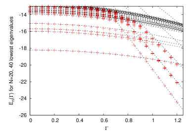
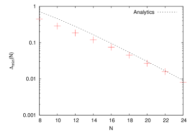
Figure 2: Left: Evolution of lowest energy levels for a single realization of the QREM with $N=20$ spins (dots) compared with analytical predictions (lines). The $40$ lower eigenvalues are evaluated via Lanczos iteration. Right: Evolution of the ensemble averaged minimal Gap at the transition, together with the asymptotic analytical prediction.

3 Numerical simulations

The matrix elements of ${\cal{H}}_{0}^{\alpha\alpha}=E_{\alpha}$ and ${\cal{H}}_{0}^{\alpha\neq\beta}=0$, while $V_{\alpha\beta}=1$ if $\alpha$ and $\beta$ are two configurations that differ by a single spin flip and zero otherwise. ${\cal{H}}$ is sparse and can be studied numerically rather efficiently even for large system sizes using Arnoldi and Ritz methods [22]. We thus have performed a set of numerical studies on these matrices, until $N=24$. We shows our results in FIG.2 and FIG.3.

The prediction for the closure of the gap as $\Delta_{min}(N)=2|E_{o}|2^{-N/2}$ compares very well with numerical simulation, even for small numbers of spins (see FIG.2.). Notice, however, that there are strong fluctuations from sample to sample (see FIG.3).

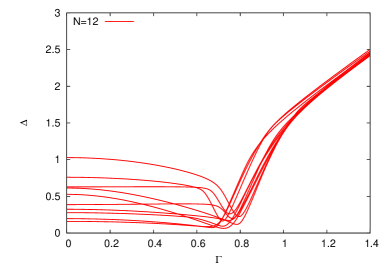
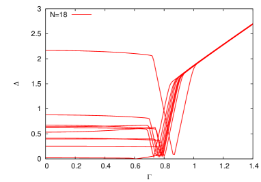
Figure 3: Energy gaps between the ground state and the first excited state in the QREM for $10$ realizations for $N=12$ (left) and $N=18$ (right). Notice the strong fluctuations between samples. As $N$ grows, the region where the gap closes shrinks and the slope around the critical point is growing dramatically. This shows that one has to be extremely cautious when performing simulation in this region.

4 Computing the gap in the generic case within the replica method

The usual way of computing the free energy of a quantum spin system is to start with the trace $Tr[e^{-\beta H}]$. One works in imaginary time and uses a a Suzuki-Trotter decomposition [18, 25, 26, 27]. In this way one obtains an ansatz for the spin-glass phase, and a different one for the quantum paramagnetic phase, yielding free energies $F_{SG}$ and $F_{QP}$, respectively through $-\beta F_{SG}\sim\ln Tr[e^{-\beta H}]$ or $-\beta F_{QP}\sim\ln Tr[e^{-\beta H}]$, depending on the phase.

Consider now the situation with the system near the phase transition, having two almost degenerate ground states $|SG\rangle$ and $|QP\rangle$, $H_{SG}=\langle SG|H|SG\rangle\sim H_{QP}=\langle QP|H|QP\rangle$ and a small interaction matrix element $H_{I}=\langle QP|H|SG\rangle$. To obtain the gap between levels, we have already diagonalized this $2\times 2$ matrix exactly in the previous section. Alternatively, we can use the classical expansion:

$$Tr[e^{-\beta H}]=\sum_{r}\frac{1}{r!}\int dt_{1}...dt_{r}e^{-\left[t_{tot}^{SG}H_{SG}+t_{tot}^{QP}H_{QP}\right]}\;\{H_{I}\}^{r}$$ (12)

where the system jumps at times $t_{1},...,t_{r}$ between the states $|SG\rangle$ and $|QP\rangle$, $t_{tot}^{SG}$ and $t_{tot}^{QP}=\beta-t_{tot}^{SG}$ denote the total time spent in each state.

What equation (12) tells us is that if we find a solution in imaginary time that interpolates between the quantum paramagnet and the spin-glass solutions by jumping $r$ times, $t_{1},...,t_{r}$, and we find that the free energy has a value:

$$\beta F_{\{r\;jumps\}}\sim t_{tot}^{SG}F_{SG}+t_{tot}^{QP}F_{QP}-rG({\mbox{interface}})$$ (13)

then by simple comparison $\ln H_{I}\sim G({\mbox{interface}})$ leading to ${\mbox{gap}}\sim e^{G}$. An extensive value of $G$ for the interface implies an exponentially small matrix element, and hence an exponentially small gap. We shall now show that this is the situation for all models of the ‘Random First Order’ kind. Indeed, this is just the usual instanton construction, the difference here will be that they take a rather unusual two-time form in problems with disorder.

Let us look for solutions interpolating between vacua. We consider the p-spin model in transverse field and shall follow the presentation and notation of Obuchi, Nishimori and Sherrington [23]. The Hamiltonian is:

$${\cal H} = -\sum_{i_{1},\ldots,i_{p}}J_{i_{1},\ldots,i_{p}}\sigma^{z}_{i_{1}}\ldots\sigma^{z}_{i_{p}}-\Gamma\sum_{i}\sigma_{i}^{x}$$ (15)

$${\rm with}~{}~{}~{}P(J_{i_{1},\ldots,i_{p}})=\left(\frac{N^{p-1}}{\pi p!}\right)^{1/2}e^{-\frac{J_{i_{1},\ldots,i_{p}}^{2}}{p!}N^{p-1}}$$

In order to solve the system, we first apply the Trotter decomposition in order to reduce the problem to a classical one with an additional “time” dimension:

$$Z=\lim_{M\rightarrow\infty}{\rm Tr}\left({\rm e}^{-\beta T/M}{\rm e}^{-\beta V/M}\right)^{M}=\lim_{M\rightarrow\infty}Z_{M},$$ (16)

where

$$Z_{M}=C^{MN}{\rm Tr}\exp\left(\frac{\beta}{M}\sum_{t=1}^{M}\sum_{i_{1}<\ldots<i_{p}}J_{i_{1}\ldots i_{p}}\sigma_{i_{1},t}\ldots\sigma_{i_{p},t}+B\sum_{t=1}^{M}\sum_{i}\sigma_{i,t}\sigma_{i,t+1}\right),$$ (17)

and we have introduced the constants $B=\frac{1}{2}\ln\coth\frac{\beta\Gamma}{M}$ and $C=\left(\frac{1}{2}\sinh\frac{2\beta\Gamma}{M}\right)^{\frac{1}{2}}$.

Replicating $n$ times, and carrying over the averages over the interactions, we get:

$$\left[Z^{n}_{M}\right]\propto{\rm Tr}\exp\Biggl{(}\frac{\beta^{2}J^{2}N}{4M^{2}}\sum_{t,t^{\prime}=1}^{M}\sum_{\mu,\nu=1}^{n}\left(\frac{1}{N}\sum_{i}\sigma_{i,t}^{\mu}\sigma_{i,t^{\prime}}^{\nu}\right)^{p}+B\sum_{t=1}^{M}\sum_{\mu=1}^{n}\sum_{i}\sigma_{i,t}^{\mu}\sigma_{i,t+1}^{\mu}\Biggr{)},$$

where the replica indices are denoted by $\mu$ and $\nu$.

In order to solve problem, it is then necessary to introduce a time-dependent order parameter $q_{tt^{\prime}}^{\mu\nu}$ and its conjugate Lagrange multiplier ${\widetilde{q}_{tt^{\prime}}^{\mu\nu}}$ for the constraint $q_{tt^{\prime}}^{\mu\nu}=\sum_{i}\sigma_{i,t}^{\mu}\sigma_{i,t^{\prime}}^{\nu}/N$. With these notations, the replicated trace reads:

$$\left[Z^{n}_{M}\right]=e^{-N\beta F}=\int\prod_{\mu<\nu}\prod_{t,t^{\prime}}dq_{tt^{\prime}}^{\mu\nu}d{\widetilde{q}_{tt^{\prime}}^{\mu\nu}}\prod_{\mu}\prod_{t\neq t^{\prime}}dq_{tt^{\prime}}^{\mu\mu}d{\widetilde{q}_{tt^{\prime}}^{\mu\mu}}$$

$$\times\exp N\Biggl{\{}\sum_{t,t^{\prime}}\sum_{\mu<\nu}\left(\frac{\beta^{2}J^{2}}{2M^{2}}\left(q_{tt^{\prime}}^{\mu\nu}\right)^{p}-\frac{1}{M^{2}}{\widetilde{q}_{tt^{\prime}}^{\mu\nu}}q_{tt^{\prime}}^{\mu\nu}\right)$$

$$+\sum_{t,t^{\prime}}\sum_{\mu}\left(\frac{\beta^{2}J^{2}}{4M^{2}}\left(q_{tt^{\prime}}^{\mu\mu}\right)^{p}-\frac{1}{M^{2}}{\widetilde{q}_{tt^{\prime}}^{\mu\mu}}q_{tt^{\prime}}^{\mu\mu}\right)+W_{o}\Biggr{\}}$$ (18)

where $W_{o}=\log{\rm Tr}\exp\left(-H_{{\rm eff}}\right)$, and:

$$H_{{\rm eff}}=-B\sum_{t}\sum_{\mu}\sigma_{t}^{\mu}\sigma_{t+1}^{\mu}-\frac{1}{M^{2}}\sum_{\mu<\nu}\sum_{t,t^{\prime}}{\widetilde{q}^{\mu\nu}_{tt^{\prime}}}\sigma_{t}^{\mu}\sigma_{t^{\prime}}^{\nu}$$

$$-\frac{1}{M^{2}}\sum_{\mu}\sum_{t\neq t^{\prime}}{\widetilde{q}^{\mu\mu}_{tt^{\prime}}}\sigma_{t}^{\mu}\sigma_{t^{\prime}}^{\mu}.$$ (19)

We calculate the free energy of the replicated system in the thermodynamic limit by the saddle-point method:

$$q_{tt^{\prime}}^{\mu\nu}=\langle\sigma_{t}^{\mu}\sigma_{t^{\prime}}^{\nu}\rangle\ \ {\widetilde{q}_{tt^{\prime}}^{\mu\nu}}=\frac{1}{2}\beta^{2}J^{2}p(q_{tt^{\prime}}^{\mu\nu})^{p-1},$$ ,

$$q_{tt^{\prime}}^{\mu\mu}=\langle\sigma_{t}^{\mu}\sigma_{t^{\prime}}^{\mu}\rangle\ \ {\widetilde{q}_{tt^{\prime}}^{\mu\mu}}=\frac{1}{4}\beta^{2}J^{2}p(q_{tt^{\prime}}^{\mu\mu})^{p-1}$$ , (20)

The brackets $\langle\cdots\rangle$ denote the average with the weight $\exp(-H_{{\rm eff}})$.

We now make the one-step replica symmetry broken ansatz: for every $(t,t^{\prime})$ the parameter $q_{tt^{\prime}}^{\mu\nu}$ is as in Fig 4.

Figure 4: The one-step replica symmetry breaking ansatz. The two-time two-replica overlap $q_{tt^{\prime}}^{\mu\nu}$ has the following structure. We divide replica in m groups and the overlap between replica in different group is zero while the overlap between replicas of the same group is $q_{tt^{\prime}}$ if the replica are different ($/mu\neq\nu$), are $q^{d}_{tt^{\prime}}$ is the replica are the same ($\mu=\nu$ on the diagonal).

Within the 1RSB ansatz, the replicated free energy reads:

$$-\beta f = \int dt\;dt^{\prime}\;\left\{-\frac{\beta^{2}J^{2}}{4}(1-m)q^{p}_{tt^{\prime}}\right.$$ (21)

$$+\left.\frac{1}{2}(1-m)\tilde{q}_{tt^{\prime}}q_{tt^{\prime}}+\frac{\beta^{2}J^{2}}{4}[q^{d}_{tt^{\prime}}]^{p}-\tilde{q}^{d}_{tt^{\prime}}q^{d}_{tt^{\prime}}\right\}-W_{o}[q^{d}_{t^{\prime}t^{\prime}},q_{tt^{\prime}}]$$

Up to here we have followed the standard steps [18, 25, 26, 27, 23] Solutions within this ansatz corresponding to the spin glass and the quantum paramagnet have been studied by several authors [18, 25, 26, 27, 23]. It turns out that the phenomenology for finite the $p$ is very close to that of the QREM.

We now part company with the previous literature, and consider a solution corresponding to the high-$\Gamma$ phase in the interval $(0,t_{1})$, $(t_{2},t_{3})$,…, that jumps to the low-$\Gamma$ phase where it stays in the intervals $(t_{1},t_{2})$, $(t_{4},t_{5})$,…. The time-dependence of $q_{t,t^{\prime}}$ and $q^{d}_{t,t^{\prime}}$ are is as in Fig. (5).

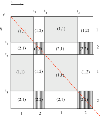
Figure 5: A multi-instanton configuration for $q^{d}_{t,t^{\prime}}$, $q_{t,t^{\prime}}$, ${\tilde{q}}^{d}_{t,t^{\prime}}$ and $\tilde{q}_{t,t^{\prime}}$. Three different shadings correspond situations in which the system is in the glass phase at both times, the paramagnetic phase at both times and in a different phase at each time. In general, the functions $q_{t,t^{\prime}}$, $\tilde{q}_{t,t^{\prime}}$ are approximately constant well within each region, with smooth, finite width interfaces. The diagonal elements $q^{d}_{t,t^{\prime}}$ and ${\tilde{q}}^{d}_{t,t^{\prime}}$ have an additional crest along the diagonal $t=t^{\prime}$. In the large $p$ limit, we may neglect this crest, in the so-called ‘static approximation’. In addition ${\tilde{q}}^{d}_{t,t^{\prime}}$ and $\tilde{q}_{t,t^{\prime}}$ become either infinity or zero, with sharp interfaces: this allows for a complete solution at large $p$.

4.1 Recovering the REM result

Let us now specialize to the large-$p$ situation, and we shall later indicate how to proceed in general. Following Obuchi et al., we note the saddle point equations imply that for large $p$ either $(q_{tt^{\prime}},q^{d}_{tt^{\prime}},\tilde{q}_{tt^{\prime}},\tilde{q}^{d}_{tt^{\prime}})=(1,1,\infty,\infty)$ or $(q_{tt^{\prime}},q^{d}_{tt^{\prime}},\tilde{q}_{tt^{\prime}},\tilde{q}^{d}_{tt^{\prime}})=(<1,<1,0,0))$. This implies that the form of the instanton configuration of $\tilde{q}^{d}_{tt^{\prime}}$ and $\tilde{q}_{tt^{\prime}}$ is the same as the one of $(q_{tt^{\prime}},q^{d}_{tt^{\prime}}$ but with the values jumping from zero to infinity. If in addition we make the ‘Static approximation’ that as applied to this case consists of assuming that inside each block the order parameters $q^{d}$ and $\tilde{q}^{d}$ are constant, we conclude that for all times we can write the ‘tilde’ variables as:

$$2\tilde{q}^{d}_{t^{\prime}t^{\prime}}-\tilde{q}_{t^{\prime}t^{\prime}}=r^{d}_{t}r^{d}_{t^{\prime}}\qquad;\qquad\tilde{q}_{t^{\prime}t^{\prime}}=r_{t}r_{t^{\prime}}$$ (22)

where $r_{t}$ and $r^{d}_{t}$ are large in the time intervals when the system is in the glass state, and drop to zero when it is not. (The solutions in the literature correspond to time-independent $r$, taking a value corresponding to either the glass or the paramagnetic phase)

Because $q^{d}_{t^{\prime}t^{\prime}},q_{t^{\prime}t^{\prime}}$ are either zero or one, we can write:

$$\int dt\;dt^{\prime}\;q_{tt^{\prime}}\tilde{q}_{tt^{\prime}} \sim \left[\int dt\;r(t)\right]^{2}=I^{2}$$

$$2\int dt\;dt^{\prime}\;\tilde{q}_{tt^{\prime}}\tilde{q}^{d}_{tt^{\prime}} = \int dt\;dt^{\prime}\;[r^{d}(t)r^{d}(t^{\prime})+r(t)r(t^{\prime})]=I_{d}^{2}+I^{2}$$ (23)

with the definitions $I\equiv\int dt\;r(t)$ and $I_{d}\equiv\int dt\;r^{d}(t)$.

We further decouple the replicas in the single-spin term in the usual way:

$$W_{o} = \log{\rm Tr}\exp\left(-H_{{\rm eff}}\right)=-\frac{1}{m}\log\left\{\int Dz_{2}\left[\int Dz_{3}\;\right.\right.$$ (24)

$$\left.\left.{\rm Tr}\left(e^{-B\sum_{t}\sigma_{t}\sigma_{t+1}-\frac{1}{M}\sum_{t}(z_{2}r_{t}+z_{3}r^{d}_{t})\sigma_{t}}\right)\right]^{m}\right\}$$

We can go back to the quantum representation, to write the trace in (24) as a single quantum-spin in a time-dependent field:

$${\rm Tr}\left({\cal{T}}e^{\int dt^{\prime}(A(t^{\prime})\sigma^{z}+\beta\Gamma\sigma^{x})}\right)$$ (25)

where ${\cal{T}}$ denotes time-order (a necessity here because of the time-dependence in the exponent) , and $A(t)\equiv(z_{3}r^{d}_{t}+z_{2}r_{t})$. In the periods where $A$ is non zero, it has a large real part and the spins are polarized along the $z$ direction. During the periods when $r_{t}=r^{d}_{t}=A=0$ only the transverse term proportional to $\Gamma$ plays a role. This corresponds to the switching between spin-glass and quantum paramagnetic phases, respectively. The trace can be computed easily by changing bases accordingly. At low temperatures, the ‘field’ in the $x$ direction $\beta\Gamma$ is strong, while the field in the $z$ direction $|A(t)|$ is either zero or $|A(t)|>>\beta\Gamma$ (for large $p$, cf. Eq. (20)). We conclude then that only one polarization of the spin contributes in each time interval. Denoting

$${\rm Tr}\left(e^{\int dt^{\prime}(A(t^{\prime})\sigma^{z}+\beta\Gamma\sigma^{x})}\right)\sim\langle z_{1}|e^{\int_{t_{n}}^{t_{f}}dt^{\prime}A(t^{\prime})\sigma^{z}}|z_{1}\rangle\langle z_{1}|x\rangle$$

$$\langle x|e^{\beta(t_{n}-t_{n-1})\Gamma\sigma^{x}}|x\rangle\;\langle x|z_{2}\rangle\;\dots\;\langle z_{n}|e^{\int_{t_{1}}^{0}dt^{\prime}A(t^{\prime})\sigma^{z}}|z_{n}\rangle$$ (26)

Where we have defined $|x\rangle$ the lowest eigenvalue of $\sigma^{x}$, and the $|z_{i}\rangle$ are either the lowest or the highest eigenvalue of $\sigma^{z}$, depending on the sign of $A(t)$ (which in turn depends on $z_{2}$,$z_{3}$) during that interval. Because, as mentioned above, at each time only one field dominates, and the way we chose the $|z_{i}\rangle$, we have:

$$\langle z_{i}|e^{\int_{t_{n}}^{t_{f}}dt^{\prime}A(t^{\prime})\sigma^{z}}|z_{i}\rangle\sim e^{\int_{t_{n}}^{t_{f}}dt^{\prime}|A(t^{\prime})|}$$ (27)

and

$$\langle x|e^{\beta\Gamma\sigma^{x}}|x\rangle\sim e^{\beta\Gamma}$$ (28)

Hence, if we denote $t^{SG}=\Theta\beta$ the total time in which $r_{t}$, $r^{d}_{t}$ are not zero, and $q_{t}=q^{d}_{t}=1$, and $t^{QP}=(1-\Theta)\beta$ the rest, the action becomes:

$$-\beta f = \Theta^{2}\;\left\{-\frac{\beta^{2}J^{2}}{4}(1-m)+\frac{\beta^{2}J^{2}}{4}\right\}-\frac{1}{2}I_{d}^{2}-\frac{m}{2}I^{2}W_{z}$$ (29)

$$+ (1-\Theta)\beta\Gamma+{\mbox{(numb. of jumps)}}\times\ln|\langle x|z\rangle|$$

where

$$W_{z} = -\frac{1}{m}\log\left\{\int Dz_{2}\left[\int Dz_{3}\;e^{\int dt|z_{2}r_{t}+z_{3}r^{d}_{t}|}\right]^{m}\right\}$$

$$= -\frac{1}{m}\log\left\{\int Dz_{2}\left[\int Dz_{3}\;e^{|z_{2}I+z_{3}I_{d}|}\right]^{m}\right\}$$

This can be evaluated by saddle point [18, 23], putting $z_{3}=I_{d}y_{3}$ and $z_{2}=Iy_{2}$ and recognizing that $I,I_{d}$ are large. There are two saddle points: $(y_{2}=1,y_{3}=1)$ and $(y_{2}=-1,y_{3}=-1)$ with the same contribution. A short calculation yields:

$$W_{z}\sim\frac{1}{2}I_{d}^{2}+\frac{m}{2}I^{2}+\ln(2)$$ (30)

Equation (29) becomes

$$-\beta f=m\Theta^{2}\frac{\beta^{2}J^{2}}{4}-\frac{\ln(2)}{m}+(1-\Theta)\beta\Gamma+{\mbox{(numb. of jumps)}}\times\ln|\langle x|z\rangle|$$ (31)

Taking saddle point with respect to $m$ gives $m=\frac{2\sqrt{2}}{\Theta\beta J}$. We finally obtain

$$-\beta f=\Theta\sqrt{\ln(2)}\frac{\beta J}{2}+(1-\Theta)\beta\Gamma+{\mbox{(numb. of jumps)}}\times\ln|\langle x|z\rangle|$$ (32)

This formula is of the form (13). It gives the contribution to $Tr[e^{-\beta H}]$ of the process with a number of jumps spending a fraction $\Theta$ in the glass state and $(1-\Theta)$ in the paramagnetic state. We have hence showed that the logarithm of matrix element is indeed the single-spin element $\sim N\ln|\langle x|z\rangle|=-N\ln(2)$ from which we recover the gap $\sim 2^{-N}$ obtained previously.

4.2 The general case

In the general case, we need to determine the functions $q^{d}_{tt^{\prime}}$ and $q_{tt^{\prime}}$ for the interval $0<t,t^{\prime}<\beta$. It suffices to compute a single jump solution, and to calculate the free energy cost of the ”wall” in the two times. This may be done numerically, discretizing the times (i.e. working in a two-time grid) and minimizing with respect to $q_{tt^{\prime}}$ while maximizing with respect to the diagonal replica parameters $q^{d}_{tt^{\prime}}$, as is usual in the replica trick.

The solution must be such that the order parameters $q^{d}_{tt^{\prime}}$ and $q_{tt^{\prime}}$ are for small $t,t^{\prime}$ close to those computed for the quantum paramagnet, for $t,t^{\prime}$ near $\beta$ close to the solution for the glass phase, and for mixed times (one large and one small) a constant corresponding to the phase-space overlap between both phases — typically zero.

At precisely the values of parameters such that the free energies of both pure solutions coincide, we have an extra free energy density cost is due exclusively the (smooth) walls separating the four quadrants in the two-time plane. Their precise form, and their free energy cost, has to be determined numerically. If their cost in free energy density is larger than zero, this is the value of the exponential dependence in the gap.

An interesting situation arises in models where the one-step replica symmetry breaking ansatz for the pure quantum phases is not exact, such as the quantum Sherrington-Kirkpatrick model. In that case, we should generalize the ansatz to allow a full replica symmetry breaking. This will not be the end of the story in such models, as the cost of the wall in the two-time plane may vanish to leading order in $N$, reflecting the fact that barriers are subextensive in height and equilibrium states are at all possible distances. In such cases, one should compute the free energy of an instanton solution scaling slower than the system size, i.e. the subextensive corrections. This is beyond our present technical capabilities.

5 Discussion

We have described an analytic technique to compute the minimal gap between the two lower quantum levels of a class of mean-field glass problems. The nature of the solution suggests that all models having the ”Random First Order” phenomenology will have an exponentially small gap, implying that quantum annealing cannot find the ground state in subexponential time. The same two-time instanton technique may be generalized to ”dilute” systems, where the connectivity is finite but locally tree-like and it would thus be interesting to adapt it to the cavity setting developed in [28]. The reader interested in seeing how the computation works in a simpler setting, in absence of disorder, is referred to [29].

Notice also that over the last few months, the first order transition scenario has been confirmed by numerical simulations in [30] as well as with analytical results in diluted systems [31].

References

- [1] S. Kirkpatrick, C.D. Gelatt and M.P. Vecchi, Science 220:671 - 680 (1983).
- [2] A.B. Finnila et al., Chem. Phys. Lett. 219, 343 (1994). T. Kadowaki and H. Nishimori, Phys. Rev. E 58, 5355 (1998). E. Farhi et al., Science 292:472 (2001). Santoro GE, Martonak R, Tosatti E, et al. Science 295 2427-2430 (2002)
- [3] Farhi E, Gutmann S Phys Rev A 57 2403 (1998)
- [4] A short version of this work has appeared in: T. Jörg, F. Krzakala, J. Kurchan and A. C. Maggs, Phys. Rev. Lett. 101 147204 (2008).
- [5] A.P. Young, S. Knysh, V. N. Smelyanskiy Phys. Rev. Lett. 101, 170503 (2008)
- [6] J. Brooke J et al., Science 284:779 (1999). J. Brooke et al., Nature, 413:610 (2001).
- [7] Grover L.K. Proceedings, 28th Annual ACM Symposium on the Theory of Computing, (1996) 212
- [8] Valkin A, Ovadyahu Z, Pollak M (2000) Phys. Rev. Lett. 84:3402. Rogge S, Natelson D, Osheroff DD (1996) Phys. Rev. Lett. 76:3136.
- [9] B. Derrida, Phys. Rev. Lett. 45, 79 (1980) and Phys. Rev. B 24, 2613 (1981).
- [10] M. Mézard, G. Parisi and M.A. Virasoro Spin Glass Theory and Beyond, World Scientific Singapure (1984).
- [11] D. J. Gross and M. Mézard, Nuclear Physics B, 240 4 431 (1984).
- [12] T. Kirkpatrick and D. Thirumalai, Phys. Rev. Lett. 58, 2091 (1987); T. Kirkpatrick, P. Wolynes, Phys. Rev. A 35, 3072 (1987).
- [13] J. Roland and N.J. Cerf, Phys. Rev. A 65, 042308 (2002). R. D. Somma et al., arXiv:0804.1571.
- [14] J. D. BrynXgelson and P. G. Wolynes, Proc. Natl. Acad. Sci. 84, 7524 (1987). E. Shakhnovich and A. Gutin, Biophys. Chem. 34, 187 (1989); J. Phys. A 22, 1647 (1989)
- [15] M. Mézard, G. Parisi and R. Zecchina, Science 297, 812 (2002). F. Krzakala et al., Proc. Natl. Acad. Sci. 104, 10318 (2007). T. Mora and L. Zdeborová, J. Stat. Phys. 131, 6 (2008).
- [16] M. Mézard, G. Parisi and R. Zecchina, (2002) Science 297, 812–815.
- [17] M. Mézard and A. Montanari, Information, Physics and Computation, Oxford press 2009.
- [18] Y. Y. Goldschmidt, Phys. Rev. B 41, 4858 (1990).
- [19] V Dobrosavljevic and D Thirumalai, J. Phys. A: Math. Gen. 23 L767-L774, 1990.
- [20] N. March, W. Young, and S. Sampanthan, The Many-Body Problem in Quantum Theory (Cambridge University Press, Cambridge, England, 1967).
- [21] Within each degenerate subspace the perturbation acts as a random orthogonal matrix of variance . This is tiny and weakly lifts the degeneracy.
- [22] D. C. Sorenson, SIAM J. Matrix Anal. Appl. 13, 357 (1992); T. Kalkreuter and H. Simma, Comput. Phys. Commun. 93, 33 (1996).
- [23] T. Obuchi, H. Nishimori, and D. Sherrington, J. Phys. Soc. Jpn. 76 (2007) 054002, D. B. Saakyan: Teor. Math. Fiz. 94 (1993) 173. J. Inoue: in Quantum Annealing and Related optimization Methods, ed. A. Das and B. K. Chakrabarti (Springer, Berlin, Heidelberg, 2005) Lecture Notes in Physics, Vol. 679, p. 259.
- [24] E. Schrodinger, Annalen der Physik, Vierte Folge, Band 80, p. 437 (1926); L. D. Landau and E. M. Lifschitz, ”Quantum Mechanics: Non-relativistic Theory”, 3rd ed.
- [25] T. M. Nieuwenhuizen and F. Ritort, Physica A, 250, 1, 8-45 (1998).
- [26] G. Biroli and L. F. Cugliandolo, Phys. Rev. B 64, 014206 (2001).
- [27] Leticia F. Cugliandolo et al., Phys. Rev. Lett. 85, 2589 - 2592 (2000) and Phys. Rev. B 64, 014403 (2001).
- [28] F. Krzakala, A. Rosso, G. Semerjian and F. Zamponi Phys. Rev. B 78, 134428 (2008).
- [29] T. Jörg, F. Krzakala, J. Kurchan, A. C. Maggs and J. Pujos, in preparation.
- [30] A. P. Young, S. Knysh, V. N. Smelyanskiy, arXiv:0910.1378.
- [31] T. Jörg, F. Krzakala, G. Semerjian and F. Zamponi, in preparation.