The Widom-Rowlinson mixture on a sphere : Elimination of exponential slowing down at first-order phase transitions

Abstract

Computer simulations of first-order phase transitions using “standard” toroidal boundary conditions are generally hampered by exponential slowing down. This is partly due to interface formation, and partly due to shape transitions. The latter occur when droplets become large such that they self-interact through the periodic boundaries. On a spherical simulation topology, however, shape transitions are absent. By using an appropriate bias function, we expect that exponential slowing down can be largely eliminated. In this work, these ideas are applied to the two-dimensional Widom-Rowlinson mixture confined to the surface of a sphere. Indeed, on the sphere, we find that the number of Monte Carlo steps needed to sample a first-order phase transition does not increase exponentially with system size, but rather as a power law $\tau\propto V^{\alpha}$, with $\alpha\approx 2.5$, and $V$ the system area. This is remarkably close to a random walk for which $\alpha_{\rm RW}=2$. The benefit of this improved scaling behavior for biased sampling methods, such as the Wang-Landau algorithm, is investigated in detail.

I Introduction

Figure 1: Phase separation snapshots of the 2D WR mixture as obtained in grand canonical MC simulations using “standard” toroidal boundary conditions, i.e. a square with periodic boundaries. The snapshots were obtained at fugacity $z=2.5$, which is well above the critical fugacity $z_{\rm cr}$, and so the transition is strongly first-order here. The light regions correspond to the vapor phase, dark regions to the liquid phase. Starting in the vapor phase (a), a droplet of liquid nucleates (b). The droplet grows until the strip configuration is reached (c). Further increasing the amount of liquid phase leads to a droplet of vapor (d), and finally this droplet vanishes, leading to the pure liquid phase (e).

Phase transitions in colloidal suspensions are of profound practical interest. Think, for instance, of phase separation in colloid-polymer mixtures aarts.schmidt.ea:2004 , or the freezing of colloidal hard spheres at high densities poon:2004 . For this reason, there is also an enormous interest in the modeling of phase transitions by means of computer simulation. The investigation of phase transitions via computer simulation is not trivial, as there are numerous hurdles to overcome. One obvious problem is the issue of finite system size. Since computational resources are limited, one always deals with finite numbers of particles, whereas phase transitions are defined in the thermodynamic limit. Hence, there is an obvious “gap” to bridge, achieved in practice using finite-size scaling fsslit .

Another problem, which we focus on in the present paper, concerns exponential slowing down, and affects simulations of first-order phase transitions berg.neuhaus:1992 . To illustrate the problem we consider phase separation in the Widom-Rowlinson (WR) mixture widom.rowlinson:1970 in two dimensions (2D). In this model there are two particle species, A and B, each modeled as disks of diameter $a$ (in what follows $a$ will be the unit of length). The only interaction is a hard-core repulsion between A and B disks. As is well known, the WR mixture phase separates provided the fugacities $z_{A}$ and $z_{B}$, of A and B particles, are high enough; due to symmetry it holds that $z_{A}=z_{B}\equiv z$ at the transition, which we shall use throughout this work. When phase separation occurs, one obtains a “vapor” phase (dense in B species, and lean in A species) and a “liquid” phase (lean in B species, and dense in A species). The particle density of A species $\rho_{A}=N_{A}/V$ may be used as order parameter to distinguish between the phases, since it assumes a low value in the vapor phase, and a high value in the liquid. Here, $N_{A}$ is the number of A particles in the system, and $V$ the total system area (the choice for A or B is arbitrary, of course). Despite its simplicity, the 2D WR mixture is relevant for phase separation in cell membranes, as the latter also constitute effectively 2D systems (which even give rise to 2D Ising critical exponents citeulike:3850776 ).

The standard approach to simulate the 2D WR mixture is to perform a grand canonical Monte Carlo (MC) simulation on a $V=L\times L$ square with periodic boundaries. Provided the fugacity $z$ significantly exceeds the critical value $z_{\rm cr}$, such that the transition is first-order, phase separation proceeds as shown in Fig. 1 citeulike:5076327 ; citeulike:4503186 . Starting in the vapor phase (a), a nucleation event occurs, leading to the condensation of a droplet of the liquid phase (b). The droplet grows until it interacts with itself through the periodic boundaries, leading to the strip configuration (c). In the strip configuration, vapor and liquid coexist with each other, separated by two interfaces that run perpendicular to one of the edges of the simulation square as this minimizes the interfacial area. The approach to the liquid proceeds via the formation of a vapor droplet (d), which eventually vanishes, leading to a pure liquid phase (e).

The path connecting vapor and liquid thus passes the strip configuration of Fig. 1(c). However, in a standard MC simulation, where configurations appear proportional to their Boltzmann weight, the strip configuration is extremely rare, due to the large amount of interface that it contains. In 2D, the total interface length in the strip configuration equals $2L$, corresponding to a free energy barrier $\Delta F=2\sigma L$, where $\sigma$ is the line tension. Hence, starting in one of the pure phase (a) or (e), it typically takes $\tau\sim\exp\left(2\sigma L\right)$ MC steps to reach the strip configuration. Since the “tunneling” time $\tau$ increases exponentially with the system size $L$, and hence explains the phrase “exponential slowing down”, it is clear that the standard MC method must be modified at a first-order phase transition in order to remain efficient.

Such modifications have been made, and the state-of-the-art is to not sample from the Boltzmann distribution, but from a modified distribution, such that the “unfavorable” interface configurations of Fig. 1(b,c,d) are sampled just as often as the “pure” phases (a) and (e). Crucial to these methods is the use of an order parameter, constructed such that

1. it varies strictly monotonically along the path connecting the phases, and

2. is computationally fast to calculate.

Regarding the 2D WR mixture, a convenient order parameter is the particle density $\rho_{A}$, which certainly fulfills criterion (2). In the vapor phase $\rho_{A}\equiv\rho_{\rm A,vap}$, in the liquid phase $\rho_{A}\equiv\rho_{\rm A,liq}$, while in the strip configuration $\rho_{A}\approx(\rho_{\rm A,vap}+\rho_{\rm A,liq})/2$. The idea is to perform a MC simulation using a biased energy $E_{B}=E_{0}+w(\rho_{A})$, with $E_{0}$ the original energy of the system, and $w(\rho_{A})$ some a priori unknown function of the order parameter $\rho_{A}$. Clearly, by tuning $w(\rho_{A})$ appropriately, the probability of the interface configurations can be artificially enhanced. The aim is to construct $w(\rho_{A})$ such that the simulation performs a random walk in $\rho_{A}$. Various methods can be used to construct $w(\rho_{A})$ in practice, such as multicanonical sampling berg.neuhaus:1992 , (successive) umbrella sampling citeulike:2414151 ; virnau.muller:2004 , and Wang-Landau sampling wang.landau:2001 . The methods differ in details, but all provide a means to obtain $w(\rho_{A})$.

Hence, using a suitable $w(\rho_{A})$, the free energy barrier of interface formation is eliminated, the coexistence configurations of Fig. 1(b,c,d) become accessible, and a random walk in $\rho_{A}$ will result (or so one hopes). In practice, this is not the case citeulike:4503186 because, strictly speaking, $\rho_{A}$ does not fulfill criterion (1) and hence is not a suitable order parameter. To see this, consider the case where half of the simulation square is occupied with vapor, and the other half with liquid. One way to arrange the phases is the strip configuration (c), with the distance between the interfaces being $L/2$. However, one could equally well arrange the phases in one of droplet configurations (b) or (d), with the droplet radius being $L/\sqrt{2\pi}$. Both “solutions” yield the same order parameter $\rho_{A}$, but clearly differ in topology. This is a problem because the transition from the droplet to the strip configuration is a first-order transition by itself, with a complicated order parameter not simply related to $\rho_{A}$ citeulike:4503186 . As with any first-order transition, these so-called shape transitions also lead to exponential slowing down. This means that simulations do not yield random walk behavior in the order parameter, even when $w(\rho_{A})$ is accurately known. Instead, most time is spend in the pure phases (a) and (e), or in the strip configuration (c), but transitions between the pure phases and the strip become increasingly rare with increasing system size citeulike:4503186 ; vink.schilling:2005 . This leads to poor sampling statistics in practice.

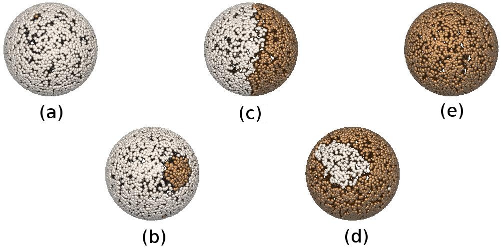
Figure 2: The analogue of Fig. 1 but this time the simulation was performed on the surface of a sphere. In contrast to toroidal boundary conditions, the transition from the vapor (a) to the liquid (e) involves only the nucleation of a droplet. Once such a droplet has formed, the path from (b) to (d) does not involve any shape transitions; the images (b), (c), and (d) only differ in the relative volume of the phases, not in their geometric configuration.

In principle, these problems can probably be overcome using a more sophisticated order parameter, one that also distinguishes between shape. However, such order parameters are not trivial to construct, and are likely to be computationally expensive, which would violate criterion (2). An alternative approach is to use a different simulation box topology, one in which shape transitions are absent citeulike:4503186 ; citeulike:5076327 . Note that the droplet-strip transition is a consequence of using a square simulation box with periodic boundaries (topologically equivalent to a torus). It is clear that on the surface of a sphere, the droplet-strip transition would not occur. Instead, on a sphere, we expect a first-order transition to proceed as shown in Fig. 2. Starting in the vapor phase (a), we still expect a nucleation event, leading to a droplet of the liquid phase (b). By increasing $\rho_{A}$ further, the droplet grows continuously (c,d) but there are no shape transitions. There is still one nucleation event, of course, as the vapor droplet (d) vanishes, leading to a pure liquid phase (e). Hence, on the surface of a sphere, shape transitions are absent, and by using an accurate bias function $w(\rho_{A})$ one should achieve behavior more closely resembling a random walk in $\rho_{A}$. In fact, any remaining slowing-down is due to nucleation, i.e. of actual physics taking place, and should prove rewarding to study further.

The primary aim of this paper is to investigate if exponential slowing-down at first-order transitions is indeed eliminated on a spherical topology. The idea of doing so was announced some time ago citeulike:5076327 , but as far as we know, such simulations have not been performed to date. In fact, we are only aware of Ref. citeulike:4503186, , which considers a 2D Ising model on the surface of a cube. The latter only crudely approximates a sphere, but already the barriers arising from shape transitions were seen to soften. Of course, being a lattice model, the extension to a spherical topology is not feasible in the Ising case. In contrast, for the 2D WR mixture, which is entirely off-lattice, the extension to a spherical topology poses no fundamental objections.

The outline of this paper is as follows. We first describe the grand canonical MC method in the presence of a bias function, and we provide some implementation details as to how this method can be efficiently implemented on the surface of a sphere. Next, we perform a number of cross-checks, to demonstrate that toroidal and spherical simulation topologies are consistent with each other in the thermodynamic limit. We then turn to our main result, and show that at first-order phase transitions, exponential slowing down on the sphere is largely eliminated. Finally, we discuss how this improved performance benefits a number of sampling algorithms, in particular the Wang-Landau algorithm. We end with some concluding remarks in the last Section.

II Methods

II.1 Grand canonical Monte Carlo

We simulate the 2D WR mixture in the grand canonical (GC) ensemble using a bias function $w(N_{A})$, i.e. defined on the number of A particles. The WR mixture was defined in the Introduction; here we only explain the GC simulation method. In the GC ensemble, the fugacity $z$ and the system area $V$ are fixed, while the number of particles fluctuates. Phase separation is studied using the order parameter distribution $P_{V}(N_{A}|z)$, defined as the probability to observe a system containing $N_{A}$ particles of type A. We emphasize that $P_{V}(N_{A}|z)$ depends on the imposed fugacity $z$, the system area $V$, and on the simulation box topology (here: toroidal or spherical). The basic MC steps used to sample the distribution are insertions and removals of single particles. At each step, the simulation attempts with equal probability one of the four following moves:

1. insertion of one A particle at a random location,

2. removal of one randomly selected A particle,

3. insertion of one B particle at a random location,

4. removal of one randomly selected B particle.

If the insertion attempts lead to forbidden overlaps, they are rejected. Otherwise, the moves are accepted with probabilities

$$p_{\text{ins,A}} = \min\left[1,\frac{zV}{N_{A}+1}e^{w(N_{A}+1)-w(N_{A})}\right],$$ (1)

$$p_{\text{rem,A}} = \min\left[1,\frac{N_{A}}{zV}e^{w(N_{A}-1)-w(N_{A})}\right],$$ (2)

$$p_{\text{ins,B}} = \min\left[1,\frac{zV}{N_{B}+1}\right],$$ (3)

$$p_{\text{rem,B}} = \min\left[1,\frac{N_{B}}{zV}\right].$$ (4)

In the above, $N_{A}$ ($N_{B}$) refers to the number of A (B) particles in the system at the start of the move. Note the presence of the bias function $w(N_{A})$ in moves involving $A$ particles. As was explained in the Introduction, the bias function is needed to overcome the free energy barrier of interface formation.

II.2 Implementation

The most CPU consuming steps are particle insertions, since here one needs to check for overlap with particles of the opposite species. We now discuss how these checks can be performed efficiently on the surface of a sphere. To simulate a total area $V$, the sphere radius must be $R=\sqrt{V/4\pi}$. The position of each particle on the sphere is stored using a 3D vector $\vec{r}=(x,y,z)$ with $|\vec{r}|=R$. This means carrying around a third coordinate but allows to eliminate time-consuming trigonometric functions. First note that the on-sphere distance $d$ between two particles $i$ and $j$ is the length of the shortest path over the sphere. This path lies on a great-circle, i.e. a circle with radius $R$. Hence, $d=R\,\theta$, where $\cos\theta=\left(\vec{r}_{i}\cdot\vec{r}_{j}\right)/R^{2}$. Unlike particles $i$ and $j$ overlap when $d<a$, with $a$ the particle diameter or, equivalently, whenever

$$\vec{r}_{i}\cdot\vec{r}_{j}>R^{2}\cos\left(a/R\right),$$ (5)

where the right-hand side is a constant, which needs to be evaluated only once at the start of the simulation. Hence, to check for overlap, only the computationally cheap term $\vec{r}_{i}\cdot\vec{r}_{j}$ is needed but no trigonometric functions.

The second optimization concerns the implementation of link-cell neighbor lists allen.tildesley:1989 on the sphere. To this end, the sphere (of radius $R$) is “embedded” in a 3D cube of edge $2R$. The cube itself is partitioned in $n\times n\times n$ equally sized sub-cubes, with $n=2R/a$ rounded down to the nearest integer. Since it holds that

$$d\geq|\vec{r}_{i}-\vec{r}_{j}|,$$ (6)

with $d$ the on-sphere distance between particles $i$ and $j$, one only needs to check for overlap with particles that are in the same sub-cube, or in any of the neighboring sub-cubes (including diagonal neighbors). Note that the number of neighboring sub-cubes that needs to be checked is typically less than the maximum of $3^{3}-1=26$ possible neighbors, since only sub-cubes actually intersecting with the surface of the sphere have to be taken into account. In practice, only about $13-14$ neighboring sub-cubes were counted in our simulations.

III Results

III.1 Order parameter distribution and line tension

Figure 3: Order parameter distribution $P_{V}(N_{A}|z)$ for the 2D WR mixture obtained at fugacity $z=2.5$ using toroidal (dashed line) and spherical (solid line) simulation topologies. Note the logarithmic scale. The system area equals $V=1600$ in both cases. Due to the high value of $z$, the vapor peak on the left is squeezed to the edge. Also indicated are the free energy barriers $\Delta F_{t}$ and $\Delta F_{s}$, which can be used to obtain the line tension $\sigma$.

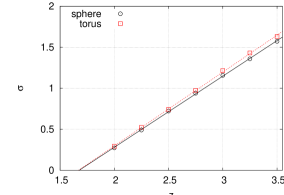
Figure 4: Variation of the line tension $\sigma$ versus $z$ as obtained using toroidal (dashed line with squares) and spherical (solid line with circles) simulation topologies. The data were obtained at fixed system area $V=1600$ in both cases, and so finite-size effects are not accounted for.

We begin our analysis by explicitly showing the order parameter distribution $P_{V}(N_{A}|z)$ as obtained using a toroidal and spherical simulation topology. Fig. 3 shows a typical result for a fugacity $z$ high above the critical fugacity $z_{\rm cr}$; the system area $V$ is the same in both cases. The distributions reveal two peaks: the left peak corresponds to the pure vapor phase, the right peak to the pure liquid, and from the peak positions $\rho_{\rm A,vap}$ and $\rho_{\rm A,liq}$ can be read-off. Whenever the simulation visits the peaks, a single homogeneous phase is observed, i.e. resembling the snapshots of Fig. 1(a,e) and Fig. 2(a,e). On the scale of the graph, the peak positions between the toroidal and spherical topology practically coincide. This is to be expected because the pure phases do not contain any interfaces. Only in the region between the peaks are differences between the two topologies expected to appear.

For the toroidal topology, a pronounced flat region between the peaks unfolds. This is where the system assumes the strip configuration of Fig. 1(c). In this configuration, an increase of the volume of either phase at the expense of the other phase merely moves the interface but does not change its form nor affect the bulk phases. Hence, the free energy remains the same under such a change which is the origin of the characteristic flat region in the probability distributions of systems on a toroidal topology. Following Binder binder:1982 , the average height $\Delta F_{t}$ of the peaks above the flat region, measured in the logarithm of $P_{V}(N_{A}|z)$, corresponds to the free energy cost of interface formation. Since the total amount of interface in the strip configuration equals $2L$, one immediately obtains the line tension

$$\sigma=\Delta F_{t}/(2L)\hskip 14.22636pt\mbox{(toroidal topology)},$$ (7)

with $L$ the edge of the simulation square. In contrast, using a spherical topology, $P_{V}(N_{A}|z)$ does not reveal any flat region. The reason is that on the sphere, any change in the relative volume of the phases inevitably creates or destroys interface. The maximum amount of interface is generated when half the sphere is occupied with vapor, and the other half with liquid, i.e. conform Fig. 2(c). The interface length then equals $2\pi R$, and the analogue of Eq.(7) becomes

$$\sigma=\Delta F_{s}/(2\pi R)\hskip 14.22636pt\mbox{(spherical topology)},$$ (8)

with $R$ the sphere radius, and $\Delta F_{s}$ the barrier height. The estimates of the line tension as a function of the fugacity are shown in Fig. 4 for both topologies using $V=1600$. In agreement with theoretical expectations, $\sigma$ decreases with decreasing $z$, and at $z_{\rm cr}$ it vanishes. However, $\sigma$ obtained on the sphere is systematically below that of the torus, the discrepancy being around 5%. In principle, we only expect agreement in the thermodynamic limit, and so a detailed investigation of finite-size effects berg.hansmann.ea:1993 is required to resolve this issue. In addition, $\sigma$ obtained on the torus corresponds to planar interfaces, whereas the interfaces on the sphere are curved. Hence, there could be curvature corrections, possibly involving Tolman’s length citeulike:4609411 .

III.2 Locating the critical point

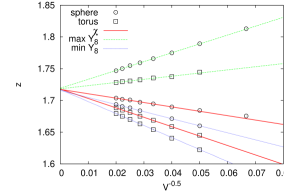
Figure 5: Determination of $z_{\rm cr}$ via finite-size scaling using both toroidal (squares) and spherical (circles) simulation topologies. Plotted are the fugacities at which $\chi$ and $Y_{8}^{\pm}$ attain their extrema versus $1/l$, with $l=\sqrt{V}$ the lateral extension of the system; the lines are linear fits. For systems of finite size, the results differ significantly between the different topologies, but agree on the value of $z_{\rm cr}$ in the thermodynamic limit.

In the thermodynamic limit, phase transition properties should not depend on the simulation topology. So as a test for the validity of using a spherical topology, rather than the more common toroidal one, we compare predictions for the critical point. Simulating at fugacities around the critical point, and using histogram reweighting ferrenberg.swendsen:1988 , we verified that in both cases the same value of the critical fugacity $z_{\rm cr}$ is obtained, as well as critical exponents consistent with 2D Ising universality. Fig. 5 shows the result of a finite-size scaling study along the lines of Ref. orkoulas.fisher.ea:2001, . For both topologies, we have plotted the fugacities at which the susceptibility $\chi$ attains its maximum versus $1/l$. Here, $l=\sqrt{V}$ denotes the “length” of the system. Also shown are the fugacities at which the generalized susceptibility $Y_{8}^{\pm}$ attains its global extrema, with $Y_{8}^{\pm}$ defined in Ref. orkoulas.fisher.ea:2001, . The lines are linear fits, which capture the data well, consistent with the exact 2D Ising value $\nu=1$ of the correlation length critical exponent. Clearly, in finite systems, the results between the two topologies differ, but both extrapolate to a common value $z_{\rm cr}=1.717(2)$ in the thermodynamic limit (the error reflects the scatter between individual scaling results). Furthermore, in both topologies, we find that the maximum value of the susceptibility increases with the length of the system as $\chi_{\rm max}\propto l^{\gamma/\nu}$, with $\gamma$ the critical exponent of the susceptibility. We obtain $\gamma_{t}\approx 1.754$ and $\gamma_{s}\approx 1.743$, for the toroidal and spherical topology, respectively, which both compare well to the exact 2D Ising value $\gamma=7/4$. Our estimate of $z_{\rm cr}$ for the 2D WR mixture is close to the one reported in Ref. johnson.gould.ea:1997, , but upon careful inspection does underestimate it (by about 0.5%). Interestingly, one of us (RV) has experienced a similar disagreement for the 3D WR mixture as well vink:2006 . The origin of the discrepancy is not clear.

III.3 The fate of exponential slowing down

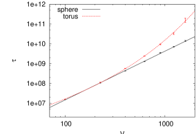
Figure 6: Main result of this paper: shown is the number $\tau$ of MC steps needed to traverse from $\rho_{A}=0$ to $\rho_{A}=3.5$ and back as a function of the system area $V$ in biased simulations using toroidal (dashed line) and spherical (solid line) boundary conditions. Note the double-logarithmic scale! The important result to take from this figure is that $\tau$ increases strongly with $V$ (presumably exponentially) on the torus, but only weakly (power law) on the sphere. The data were obtained for the 2D WR mixture at fugacity $z=2.5$; the exponent of the power law for the spherical topology equals $\alpha\approx 2.5$, which is remarkably close to $\alpha_{\rm RW}=2$ of a true random walk.

We now come to the main result of this paper, where we consider exponential slowing down at a first-order phase transition. Our hope is that, by using a spherical topology, exponential slowing down can be largely eliminated. To this end, we set the fugacity to $z=2.5$ which is well above $z_{\rm cr}$, and so the transition is strongly first-order. We remind the reader that our simulations use a bias function $w(N_{A})$ to overcome the free energy barrier of interface formation, and also that $w(N_{A})$ is a priori unknown. Hence, for a number of system sizes $V$, accurate bias functions $w(N_{A})$ were first obtained using successive umbrella sampling virnau.muller:2004 , for both toroidal and spherical topologies. Next, biased simulations were performed using the (now known) bias functions, and the number of MC steps $\tau$ needed to traverse from $\rho_{A}=0$ to $\rho_{A}=3.5$ and back was measured; the reader can verify in Fig. 3 that this range is sufficient to sample both the vapor and liquid peaks.

The resulting $\tau$ data are collected in Fig. 6. The most striking feature of the plot is that for a toroidal topology $\tau$ indeed increases faster than a power law with $V$. Following the discussion in the Introduction, we attribute this slow down to free energy barriers associated with the droplet-strip shape transition, which are not overcome by the bias function $w(N_{A})$. The data for the spherical topology, in contrast, do not reveal any exponential slow down for the system sizes considered here but rather a power law increase; approximately $\tau\sim V^{\alpha}$, with $\alpha\approx 2.5$. This is still a slow down compared to a perfect random walk, for which $\alpha_{\rm RW}=2$, but not an exponential one. Possibly, the remaining slow down is due to nucleation events. Comparing the values of $\tau$ between the two topologies, it is striking that already for system area $V=1600$, $\tau$ on a torus is ten times that of $\tau$ on a sphere.

III.4 Wang-Landau sampling

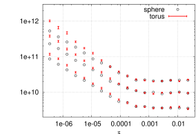
Figure 7: Number of MC moves required to complete one WL iteration, using a toroidal (vertical bars) and spherical (circles) simulation topology, on double logarithmic scales. Results are shown for system areas $V=900,1600,2500$ (bottom to top). Note that during WL sampling the larger values of $\delta$ are sampled first. The data were obtained for the 2D WR mixture at fugacity $z=2.5$.

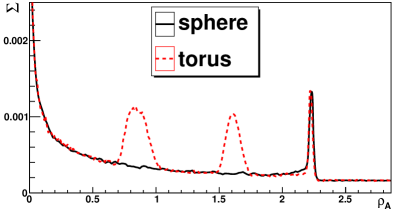
Figure 8: Variation of the statistical error $\Sigma$ in $\Delta w(N_{A})$ versus $\rho_{A}$, as obtained in WL simulations on toroidal (dashed line) and spherical (solid line) topologies. For clarity, intervals of 20 error estimates are combined to a single average. The error bars on the toroidal data represent jackknife errors for the average of this re-binning; error bars for the spherical topology are omitted. The data were obtained for the 2D WR mixture at fugacity $z=2.5$ and system area $V=2500$.

V	$\ \ \left<\rho_{A}\right>\$	$\ m_{1}\$	$\ m_{2}\$	$\ m_{3}\$	$\ m_{4}\$
900	$1.42$	$1.69$	$1.69$	$3.44$	$1.21$
1600	$2.92$	$3.83$	$3.83$	$6.51$	$3.66$
2500	$2.67$	$3.32$	$3.32$	$4.70$	$7.80$

Table 1: Relative accuracy of selected physical observables obtained using WL sampling on spherical and toroidal topologies for several system areas $V$. The ratios all exceed unity, implying that the spherical topology is to be preferred. The data were obtained for the 2D WR mixture at fugacity $z=2.5$.

Having shown that the tunneling time $\tau$ using a spherical topology can be much smaller compared to that on a torus, a natural next question is whether this improvement also increases the performance of the algorithms used to construct $w(N_{A})$. One such algorithm is Wang-Landau (WL) sampling wang.landau:2001 . Here, the bias function is initially set to $w(N_{A})=0$, and one proceeds to simulate as explained in Section II.1. Each time a state with $N_{A}$ particles of type A is visited, the corresponding value of the bias function is decreased by a modification term: $W(N_{A})\to W(N_{A})-\delta$. This reflects the idea that the current number of $A$ particles is just being found a bit more probable than previously expected and hence needs a smaller bias. One continues to simulate until all particle numbers $N_{A}$ over the range of interest have been visited sufficiently often flat , which completes one WL iteration. At this point, the modification term is reduced, say, $\delta\to\delta/2$, and the next iteration is started. By using a large modification term at first, say $\delta=1$, one ensures that all states will be visited in relatively short times. At later stages, when $\delta$ is small, changes to the bias function become negligible, and the algorithm is said to have converged. Clearly, for the performance of this algorithm, it helps if the simulation traverses the density range of interest as quickly as possible. This is obviously related to the tunneling time $\tau$, which is significantly reduced on a spherical topology, and so we expect an increased performance for WL sampling too.

To test the performance of WL sampling on toroidal and spherical topologies, the bias function $w(N_{A})$ was measured independently $40$ times using system sizes $V=900,1600,2500$ (by independent we mean that each WL run was started with its own unique stream of random numbers). In Fig. 7, the average number of MC steps needed to complete one WL iteration is plotted as a function of the modification term $\delta$. In the early stages, where $\delta$ is large, the number of MC steps is effectively identical. In this regime $\delta$ is so large that the simulations on the torus are still easily pushed through the regime of the droplet-strip transition, and hence there is no noticeable difference. However, at later stages, where $\delta$ is small, the number of required MC steps is significantly less on the sphere, as expected, since here the sphere simulations benefit from the improved diffusion behavior demonstrated in Fig. 6.

Hence, late-stage WL iterations indeed complete faster on a spherical topology, compared to a toroidal one. Next, it remains to be shown that actual physical observables are also more accurately obtained. To this end, we consider the average density of A particles ${\langle\rho_{A}\rangle}$, and the first four central moments

$$m_{n}=\left<\right.\left|\rho_{A}-\left<\rho_{A}\right>\right|^{n}\left.\right>.$$ (9)

Note that ${\langle\rho_{A}\rangle}$ and $m_{n}$ are trivially obtained from the order parameter distribution $P_{V}(N_{A}|z)$, which in turn is related to the bias function $w(N_{A})=-\log P_{V}(N_{A}|z)$. For each topology, we thus have a set of $40$ estimates per observable. Using the jackknife method newman.barkema:1999 , one can derive the statistical error $\Sigma$ in each observable, and the “best” topology is the one with the smallest $\Sigma$. In Table 1, the ratio of errors $\Sigma_{t}/\Sigma_{s}$ is shown for each observable, with $\Sigma_{t}$ ($\Sigma_{s}$) the error as obtained on the torus (sphere). The point to take from the table is that the ratios all exceed unity, meaning that the data from the spherical topology are more reliable. In combination with the findings of Fig. 7, we conclude that WL simulations on spherical topologies are overall more efficient.

Finally, we demonstrate that the enhanced performance of WL sampling on spherical topologies can indeed be attributed to the absence of the droplet-strip shape transition. To this end, we consider the difference

$$\Delta w(N_{A})\equiv w(N_{A}+1)-w(N_{A})$$ (10)

between adjacent weights. Again using the jackknife method, we estimated the statistical error $\Sigma$ in $\Delta w(N_{A})$ from the set of $40$ simulations for each topology. Plotted in Fig. 8 is $\Sigma$ versus $\rho_{A}$. The striking feature is that on the torus, $\Sigma$ displays two extra large peaks, which are completely absent on the sphere. These extra peaks in the torus data reflect the sampling difficulties arising from the droplet-strip transition. Away from the droplet-strip transitions, both topologies yield essentially the same statistical error, as expected. Note also the excellent agreement between both topologies regarding the peak on the far right of the graph: this peak reflects a sampling problem arising from nucleation, which indeed should occur in both topologies. In principle, a nucleation peak should also be visible on the far left of the graph, but due to the high fugacity used, this peak is probably squeezed onto the vertical axes.

III.5 Successive umbrella sampling

V	$\ \ \left<\rho_{A}\right>\$	$\ m_{1}\$	$\ m_{2}\$	$\ m_{3}\$	$\ m_{4}\$
900	$1.61$	$2.61$	$2.62$	$6.8$	$1.83$
1600	$3.47$	$6.34$	$6.34$	$14.6$	$2.67$
2500	$4.43$	$11$	$11.1$	$30.1$	$11.2$

Table 2: The analogue of Table 1 but this time using successive umbrella sampling virnau.muller:2004 .

Another algorithm that can be used to construct the bias function $w(N_{A})$ is successive umbrella sampling (SUS) virnau.muller:2004 . When SUS is implemented on a spherical topology we also observe an increase in performance. In Table 2, we display some typical benchmarks regarding the accuracy of a number of physical observables. Compared to WL simulations, the performance increase in SUS simulations appears to be even more pronounced. A possible explanation may be that, unlike in WL sampling, each state $N_{A}$ was simulated using the same number of MC steps for both geometries.

IV Conclusions

In conclusion, we have shown that the droplet-strip transition, which is inherent to toroidal systems undergoing a first-order phase transition, acts as barrier making simulations of large systems increasingly harder. For the 2D WR mixture investigated here, the droplet-strip transition can be easily, and at the cost of a constant fraction of CPU time, be eliminated by simulating the system on the surface of a sphere. We have shown that for WL sampling wang.landau:2001 and SUS virnau.muller:2004 , simulations on the surface of a sphere yield better results. The droplet-strip transition is a general feature, also in 3D, appearing at all first-order phase transitions studied on toroidal topologies. Hence, the use of a spherical topology is expected to be beneficial in a great number of other systems also.

The 2D implementation sketched here should quite straightforwardly extend to 3D citeulike:6008340 , and to other (short-ranged) interactions also; obvious candidates are the hard-core square-well fluid, the (cut-and-shifted) Lennard-Jones fluid, and colloid-polymer mixtures. However, models in which the pair potential is a more complicated function of the distance may require the use of computationally expensive trigonometric functions, which were successfully circumvented in the present implementation. Even so, this additional computational effort should be outbalanced by the elimination of exponential slowing down, provided the systems are large enough.

Some models may not be so easily transferable to the sphere, in particular when particle orientation comes into play. An example is the 2D Zwanzig model zwanzig:1714 of horizontally or vertically aligned hard rods. While on the torus one can uniquely speak of horizontal and vertical directions, this is prevented by the intrinsic curvature on the sphere. Note also that the advantage of using a spherical topology is to eliminate exponential slowing down at first-order transitions. Around the critical point, where the transition is continuous, we did not see much advantage using the spherical topology.

A different application where the use of a spherical topology may be beneficial is in the simulation of droplets citeulike:4503179 ; virnau.macdowell.ea:2003 ; citeulike:5076926 . One problem of using a toroidal topology is that the maximum size of the droplet that one can simulate is limited to the point where the droplet-strip transition takes place citeulike:5076926 . On a spherical topology, this problem is circumvented. Finally, we would like to point out that phase separation on the surface of a sphere is also realized experimentally in giant vesicles citeulike:6008542 ; confocal microscopy images of the latter qualitatively resemble the simulation snapshots of Fig. 2.

Acknowledgments

This work was supported by the Deutsche Forschungsgemeinschaft under the Emmy Noether program (VI 483/1-1).

References

- (1) D. G. Aarts, M. Schmidt, and H. N. Lekkerkerker, Science 304, 847 (2004).
- (2) W. C. K. Poon, Science 304, 830 (2004).
- (3) The literature on finite-size scaling is too extensive to be cited here; for a recent review on the use of such methods in soft matter systems see: R.L.C. Vink, Soft Matter, 2009, DOI: 10.1039/b912135h.
- (4) B. A. Berg and T. Neuhaus, Physical Review Letters 68, 9+ (1992).
- (5) B. Widom and J. S. Rowlinson, The Journal of Chemical Physics 52, 1670 (1970).
- (6) A. R. Honerkamp-Smith, P. Cicuta, M. D. Collins, S. L. Veatch, M. den Nijs, M. Schick, and S. L. Keller, Biophysical Journal 95, 236+ (2008).
- (7) K. Leung and R. K. P. Zia, Journal of Physics A: Mathematical and General 23, 4593 (1990).
- (8) T. Neuhaus and J. S. Hager, Journal of Statistical Physics 113, 47 (2003).
- (9) G. Torrie and J. Valleau, Journal of Computational Physics 23, 187 (1977).
- (10) P. Virnau and M. Muller, The Journal of Chemical Physics 120, 10925 (2004).
- (11) F. Wang and D. P. Landau, Physical Review Letters 86, 2050+ (2001).
- (12) R. L. C. Vink and T. Schilling, Phys. Rev. E 71, 051716 (2005).
- (13) M. P. Allen and D. J. Tildesley, Computer Simulation of Liquids (Oxford University Press, England, 1989).
- (14) K. Binder, Phys. Rev. A 25, 1699 (1982).
- (15) B. A. Berg, U. Hansmann, and T. Neuhaus, Phys. Rev. B 47, 497 (1993).
- (16) J. S. Rowlinson, Journal of Physics A: Mathematical and General 17, L357 (1984).
- (17) A. M. Ferrenberg and R. H. Swendsen, Phys. Rev. Lett. 61, 2635 (1988).
- (18) G. Orkoulas, M. E. Fisher, and A. Z. Panagiotopoulos, Physical Review E 63, 051507+ (2001).
- (19) G. Johnson, H. Gould, J. Machta, and L. K. Chayes, Physical Review Letters 79, 2612 (1997).
- (20) R. L. C. Vink, The Journal of Chemical Physics 124, 094502+ (2006).
- (21) In practice this is determined using a “flatness” criterion, see for example Ref. citeulike:278331, .
- (22) M. E. J. Newman and G. T. Barkema, Monte Carlo Methods in Statistical Physics (Clarendon Press, Oxford, 1999).
- (23) J. M. Caillol, The Journal of Chemical Physics 99, 8953 (1993).
- (24) R. Zwanzig, The Journal of Chemical Physics 39, 1714 (1963).
- (25) K. Binder, Physica A: Statistical Mechanics and its Applications 319, 99 (2003).
- (26) L. G. Macdowell, P. Virnau, M. Müller, and K. Binder, The Journal of Chemical Physics 120, 5293 (2004).
- (27) M. Schrader, P. Virnau, and K. Binder, Physical Review E (Statistical, Nonlinear, and Soft Matter Physics) 79, 061104+ (2009).
- (28) H. M. Seeger, M. Fidorra, and T. Heimburg, Macromolecular Symposia 219, 85 (2005).
- (29) F. Wang and D. P. Landau, Physical Review E 64, 056101+ (2001).