A gap in the continuous spectrum of a cylindrical waveguide with a periodic perturbation of the surface.

Abstract

It is proved that small periodic singular perturbation of a cylindrical waveguide surface may open a gap in the continuous spectrum of the Dirichlet problem for the Laplace operator. If the perturbation period is long and the caverns in the cylinder are small, the gap certainly opens.

Key words: essential spectrum, cylindrical waveguide, gaps, perturbation of surface

MSC (2000): 35P05, 47A75, 49R50.

1 Spectra of cylindrical and periodic waveguides

1.1 The cylindrical waveguide.

Let $\Omega=\omega\times\mathbb{R}$ be a cylinder with the cross-section $\omega\subset\mathbb{R}^{2}$ bounded by a simple closed contour $\partial\omega$ assumed to be $C^{\infty}$ - smooth for simplicity (cf. Remark 1 below). Interpreting $\Omega$, e. g., as an acoustic waveguide with the soft wall $\partial\Omega$, we consider the Dirichlet problem for the Helmgoltz equation

$$-\Delta_{x}v\left(x\right)=\mu v\left(x\right)\text{, }x\in\Omega\text{, }v\left(x\right)=0\text{, }x\in\partial\Omega\text{,}$$ (1.1)

where $\Delta_{x}$ is the Laplacian, $v$ the pressure, and $\mu$ a spectral parameter, proportional to square of the oscillation frequency.

It is known (cf. [1, 2]) and can be directly verified that, above a certain cut-off $\mu_{\dagger}>0$, i. e. for $\mu\geq\mu_{\dagger}$, the problem $\left(\ref{1.1}\right)$ admits a solution in the form

$$v\left(x\right)=\exp\left(\pm i\zeta z\right)V\left(y\right)$$ (1.2)

where $i$ is the imaginary unit, $z=x_{3}$ and $y=\left(y_{1},y_{2}\right)=\left(x_{1},x_{2}\right)$ while

$$M=\mu-\zeta^{2}$$ (1.3)

and $V$ are an eigenvalue and the corresponding eigenfunction of the model problem in the cross-section

$$-\Delta_{y}V\left(x\right)=MV\left(y\right)\text{, }y\in\omega\text{, }V\left(y\right)=0\text{, }y\in\partial\omega\text{.}$$ (1.4)

Let $M_{1}$ be the principal eigenvalue in the spectrum of the problem $\left(\ref{1.4}\right)$:

$$0<M_{1}<M_{2}\leq M_{3}\leq...\leq M_{k}...\rightarrow+\infty.$$ (1.5)

By the maximum principle (see, e.g., [30]), the eigenvalue $M_{1}$ is simple and the eigenfunction $V_{1}$ can be fixed such that

$$\left\|V_{1};L^{2}\left(\omega\right)\right\|=1,\text{ }V_{1}\left(y\right)>0\text{, }y\in\omega,\text{ }\partial_{n}V_{1}\left(y\right)<0,\text{ }y\in\partial\omega,$$ (1.6)

where $\partial_{n}$ stands for differentiation along the outward normal and $L^{2}\left(\omega\right)$ for the Lebesgue space. If

$$\mu\geq\mu_{\dagger}=M_{1},$$ (1.7)

then $\zeta$ is a real number in $\left(\ref{1.3}\right)$, function $\left(\ref{1.2}\right)$ does not grow or vanish as $z\rightarrow\pm\infty$ and implies a wave which oscillates in the case $\zeta\neq 0$ and stays constant in $z$ for $\zeta=0.$ In other words, the wave propagation phenomenon occurs above the cut-off $\mu_{\dagger}$.

The problem $\left(\ref{1.1}\right)$ gives rise to the unbounded positive and self-adjoint operator $A_{\Omega}$ in $L^{2}\left(\Omega\right)$ with the differential expression $-\Delta_{x}$ and the domain

$$\mathcal{D}\left(A_{\Omega}\right)=H^{2}\left(\Omega\right)\cap\mathring{H}^{1}\left(\Omega;\partial\Omega\right).$$ (1.8)

We use the standard notation for the Sobolev space and the subspace $\mathring{H}^{1}\left(\Omega;\partial\Omega\right)$ of functions in $H^{1}\left(\Omega\right)$ satisfying the Dirichlet conditions in $\left(\ref{1.1}\right)$.

The existence of the nontrivial wave $\left(\ref{1.2}\right)$ means that the point $\mu$ belongs to the continuous spectrum $\sigma_{c}\left(A_{\Omega}\right)$ of the operator $A_{\Omega}$. Indeed, multiplying $v$ with the plateau function $X_{N}$ (Figure 1) we see that

$$\left\|X_{N}v;L^{2}\left(\Omega\right)\right\|^{2}\geq 2\left(N-1\right)\text{mes}_{2}\omega,\text{ }\left\|\left(\Delta_{x}+\mu\right)\left(X_{N}v\right);L^{2}\left(\Omega\right)\right\|\leq const,\text{ }N\in\mathbf{\mathbb{N}},$$ (1.9)

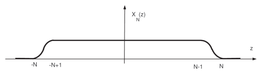
Figure 1: The plateau function

where $\mathbf{\mathbb{N}}:=\left\{1,2,...\right\},$ and, therefore, $\left\{N^{-\frac{1}{2}}X_{h}v\right\}_{N\in\mathbf{\mathbb{N}}}$ is a singular Weyl sequence of $A_{\Omega}$ at the point $\mu$ whilst $\mu$ belongs to the essential spectrum $\sigma_{e}\left(A_{\Omega}\right)$ (see, e.g. [3, §9.1]). We emphasize that, by a general result in [18] (see also [19, §3.1]), the kernel of the mapping

$$H^{2}\left(\Omega\right)\cap\mathring{H}^{1}\left(\Omega;\partial\Omega\right)\ni v\mapsto-\left(\Delta_{x}+\mu\right)v\in L^{2}\left(\Omega\right)$$ (1.10)

stays finite-dimensional for any $\mu\in\mathbf{\mathbb{C}}$ and, hence, $\sigma_{c}\left(A_{\Omega}\right)=\sigma_{e}\left(A_{\Omega}\right).$

The set $\mathbf{\mathbb{C}}\backslash\left\{\mu\in\mathbf{\mathbb{C}:\operatorname{Re}\mu\geq}\mu_{\dagger},\text{ }\operatorname{Im}\mu=0\right\}$ in the complex plane is the resolvent set of the operator $A_{\Omega}$ where the inhomogeneous Dirichlet problem

$$-\Delta_{x}v\left(x\right)-\mu v\left(x\right)=f\left(x\right),\text{ }x\in\Omega,\text{ }v\left(x\right)=0,\text{ }x\in\partial\Omega,$$ (1.11)

has a unique solution $v\in H^{2}\left(\Omega\right)$ for any right-hand side $f\in L^{2}\left(\Omega\right)$ and the attendant estimate

$$\left\|v;H^{2}\left(\Omega\right)\right\|\leq c_{\mu}\left\|f;L^{2}\left(\Omega\right)\right\|$$ (1.12)

ensures that the mapping $\left(\ref{1.7}\right)$ is an isomorphism. In contrast, on the continuous spectrum, mapping $\left(\ref{1.7}\right)$ looses even the Fredholm property (cf. [19, Thm. 3.11]) and the inhomogeneous problem $\left(\ref{1.8}\right)$ requires a specific formulation involving radiation conditions at infinity. In the sequel we do not need such the formulation and refer, e.g. to [1, 2], [19, §5.3] for details.

1.2 The periodic waveguide, a quasi-cylinder.

Let $\Pi$ be a domain in $\mathbb{R}^{3}$ with a periodic cross-section (Figure 2). More precisely, $\Pi$ is the interior of the union

$$\overline{\Pi}={\displaystyle\bigcup\nolimits_{j\in\mathbf{\mathbb{Z}}}}\overline{\varpi_{j}},$$ (1.13)

Figure 2: Periodic waveguide

where $\mathbf{\mathbb{Z}}\mathbf{=}\left\{0,\pm 1,\pm 2,...\right\},$ $\varpi_{j}=\left\{x=\left(y,z\right):\left(y,z-j\right)\in\varpi\right\},$ and the reference periodicity cell $\varpi$ lies inside the circular cylinder $\left\{x:\left|y\right|<R,\text{ }z\in\left(-\frac{1}{2},\frac{1}{2}\right)\right\}$ of radius $R>0$ and the unit height. We, of course, assume that $\Pi$ is a connected set, i.e., a domain.

Due to possible boundary irregularities the Dirichlet problem for the Helmgoltz equation in the quasi-cylinder $\Pi$ needs the variational formulation as the integral identity [17]

$$\left(\nabla_{x}u,\nabla_{x}v\right)_{\Pi}=\lambda\left(u,v\right)_{\Pi},\text{ }v\in\mathring{H}^{1}\left(\Pi;\partial\Pi\right),$$ (1.14)

where $\nabla_{x}$ is the gradient operator, $\left(\text{ },\text{ }\right)_{\Pi}$ the natural inner product in $L^{2}\left(\Pi\right)$, and $\lambda$ a spectral parameter. If the boundary $\partial\Pi$ is smooth, the integral identity $\left(\ref{1.11}\right)$ with arbitrary test function $v\in\mathring{H}^{1}\left(\Pi;\partial\Pi\right)$ is equivalent to the differential problem of type $\left(\ref{1.1}\right)$ in $\Pi$. The spectral problem reads: To find $\mu\in\mathbf{\mathbb{C}}$ and a nontrivial function $u\in\mathring{H}^{1}\left(\Omega;\partial\Omega\right)$ verifying $\left(\ref{1.11}\right).$

Remark 1

We could take any open connected and bounded cross-section $\omega$ of the cylinder $\Omega$ and formulate a spectral variational problem of type $\left(\ref{1.11}\right)$ in $\Omega$. However, the smoothness of $\partial\omega$ will be used in § 3 for an asymptotic analysis.

1.3 The band-gap structure of the essential spectrum in a quasi-cylinder.

The left-hand side of $\left(\ref{1.11}\right)$ is a positive continuous form in $\mathring{H}^{1}\left(\Pi;\partial\Pi\right)$. According to [3, §10.2], this form is associated with a positive self-adjoint unbounded operator $A_{\Pi}$ in $L^{2}\left(\Pi\right)$. If the surface $\partial\Pi$ is smooth, $A_{\Pi}$ gets the same properties as $A_{\Omega}$ with the only exception, namely, its essential spectrum has the band-gap structure

$$\sigma_{e}\left(A_{\Pi}\right)={\displaystyle\bigcup\nolimits_{p\in\mathbf{\mathbb{N}}}}\Upsilon_{p}$$ (1.15)

where $\Upsilon_{p}$ are closed segments

$$\Upsilon_{p}=\left[\Lambda_{p}^{-},\Lambda_{p}^{+}\right].$$ (1.16)

Formulas $\left(\ref{1.12}\right)$ and $\left(\ref{1.13}\right)$ remain valid without the smoothness assumption (see [10, 15] and others).

To indicate the segments $\left(\ref{1.13}\right),$ the model spectral problem on the periodicity cell $\varpi$ must be considered

$$Q_{\eta}\left(U,V;\varpi\right):=\left(\left(\nabla_{x}+i\eta e_{3}\right)U,\left(\nabla_{x}+i\eta e_{3}\right)V\right)_{\varpi}=\Lambda\left(U,V\right)_{\varpi},\text{ }V\in\mathring{H}_{per}^{1}\left(\varpi;\gamma\right),$$ (1.17)

where $e_{j}$ is the unit vector of the $x_{j}$-axis and $\mathring{H}_{per}^{1}\left(\varpi;\gamma\right)$ is the subspace of 1-periodic in $z$ functions $V\in H^{1}\left(\varpi\right)$ vanishing on the lateral side $\gamma=\left\{x\in\partial\varpi:z\in\left(-\frac{1}{2},\frac{1}{2}\right)\right\}$ of the cell. If, for certain $\eta\in\left[0,2\pi\right)$ and $\Lambda>0$, the model problem $\left(\ref{1.14}\right)$ has a nontrivial solution $U\in\mathring{H}_{per}^{1}\left(\varpi;\gamma\right)$, then the Flochet wave

$$u\left(y,z\right)=\exp\left(i\eta z\right)U\left(y,z\right)$$ (1.18)

satisfies formally the original problem in the quasi-cylinder $\Pi$ that is the integral identity $\left(\ref{1.11}\right)$ with any test function $v\in C_{c}^{\infty}\left(\overline{\Pi}\right)$ (infinitely differentiable functions with compact supports). One readily constructs from the Flochet wave the singular Weyl sequence for the operator $A_{\Pi}$ at the point $\lambda=\Lambda$ with the help of the plateau function drawn in Figure 1 (cf. formulas $\left(\ref{Weyl}\right)$).

For any real $\eta$, the sesquilinear form on the left of $\left(\ref{1.14}\right)$ is Hermitian, closed and positive. Thus, problem $\left(\ref{1.14}\right)$ can be associated with the unbounded self-adjoint positive operator $\mathcal{A}_{\Pi}\left(\eta\right)$ in $L^{2}\left(\varpi\right)$ (see again [3, §10.1]). The domain $\mathcal{D}\left(\mathcal{A}_{\Pi}\left(\eta\right)\right)$ is included into the Sobolev space $H^{1}\left(\varpi\right)$ and, therefore, is compactly embedded into $L^{2}\left(\varpi\right)$. By [3, Thm. 10.1.5], the spectrum of $\mathcal{A}_{\Pi}\left(\eta\right)$ is discrete and forms the infinitely large sequence

$$0<\Lambda_{1}\left(\eta\right)\leq\Lambda_{2}\left(\eta\right)\leq...\leq\Lambda_{p}\left(\eta\right)\leq...\rightarrow+\infty$$ (1.19)

of eigenvalues which are listed according to multiplicity. The functions $\eta\rightarrow\Lambda_{p}\left(\eta\right)$ are continuous (see [27, Ch. 9]) and, by an evident argument, $2\pi$ - periodic. This means that the endpoints of segments in $\left(\ref{1.13}\right)$ are calculated as follows:

$$\Lambda_{p}^{\pm}=\pm\max\left\{\pm\Lambda_{p}\left(\eta\right):\eta\in\left[0,2\pi\right)\right\}.$$ (1.20)

1.4 The Fourier and Gel’fand transforms.

Let us comment on the above-mentioned inference. A correspondence between the problems $\left(\ref{1.1}\right)$ in the cylinder $\Omega$ and $\left(\ref{1.4}\right)$ in the cross-section $\omega$ is pointed by the Fourier transform (see [18] and e.g. [19, 20]). For the quasi-cylinder $\Pi$, one ought to apply the discrete Fourier transform, namely, the Gel’fand transform

$$u\left(y,z\right)\longrightarrow\widehat{u}\left(y,z;\eta\right)=\frac{1}{\sqrt{2\pi}}{\displaystyle\sum\limits_{j\in\mathbf{\mathbb{Z}}}}\exp\left(-i\eta\left(z+j\right)\right)u\left(y,z+j\right)$$ (1.21)

(see [28] and e.g. [19, 15]). Note that $\left(y,z\right)\in\Pi$ on the left of $\left(\ref{1.18}\right)$ but $\left(y,z\right)\in\varpi$ on the right. The Gel’fand transform establishes the isomorphisms

$$L^{2}\left(\Pi\right)\approx L^{2}\left(0,2\pi;L^{2}\left(\varpi\right)\right),\text{ }H^{l}\left(\Pi\right)\approx L^{2}\left(0,2\pi;H_{per}^{l}\left(\varpi\right)\right)$$

where $L^{2}\left(0,2\pi;\mathfrak{B}\right)$ stands for the Lebesgue space of abstract functions,

$$\left\|U;L^{2}\left(0,2\pi;\mathfrak{B}\right)\right\|=\left({\displaystyle\int\limits_{0}^{2\pi}}\left\|U\left(\eta;\mathfrak{B}\right)\right\|^{2}d\eta\right)^{\frac{1}{2}}$$

and $\mathfrak{B}$ is a Banach space. The corresponding Parceval theorem provides the identity

$${\displaystyle\int\limits_{\Pi}}u\left(x\right)\overline{v\left(x\right)}dx={\displaystyle\int\limits_{0}^{2\pi}}{\displaystyle\int\limits_{\varpi}}\widehat{u}\left(x;\eta\right)\overline{\widehat{v}\left(x;\eta\right)}dxd\eta,\text{ }u,v\in L^{2}\left(\Pi\right),$$

which, together with the formulas

$$\widehat{v}\left(y,0;\eta\right)=\widehat{v}\left(y,1;\eta\right),\text{ }\partial_{z}\widehat{v}\left(y,z;\eta\right)=\widehat{\partial_{z}v}\left(y,z;\eta\right)-i\eta\widehat{v}\left(y,z;\eta\right),\text{ }v\in C_{c}^{\infty}\left(\overline{\Pi}\right),$$

indicate the immediate correspondence between the problem $\left(\ref{1.11}\right)$ in the quasi-cylinder $\Pi$ and the family $\left(\eta\in\left[0,2\pi\right)\right)$ of problems $\left(\ref{1.14}\right)$ in the periodicity cell $\varpi$.

A result in [16] (see also [10, 15, 19] and others) demonstrates that the operator of problem $\left(\ref{1.11}\right)$ with the fixed $\lambda\in\mathbf{\mathbb{C}}$ regarding as the mapping

$$\mathring{H}^{1}\left(\Pi;\partial\Pi\right)\longrightarrow\mathring{H}^{1}\left(\Pi;\partial\Pi\right)^{\ast}$$ (1.22)

is Fredholm if and only if, for any $\eta\in\left[0,2\pi\right)$, the problem

$$\left(\left(\nabla_{x}+i\eta e_{3}\right)U,\left(\nabla_{x}+i\eta e_{3}\right)V\right)_{\varpi}-\lambda\left(U,V\right)_{\varpi}=\mathcal{F}\left(V\right),\text{ }V\in\mathring{H}_{per}^{1}\left(\varpi;\gamma\right),$$

with the fixed $\lambda\in\mathbf{\mathbb{C}}$ is uniquely solvable with any linear functional $\mathcal{F\in}\mathring{H}_{per}^{1}\left(\varpi;\gamma\right)^{\ast}$ on the space $\mathring{H}_{per}^{1}\left(\varpi;\gamma\right)$. The fact mentioned above ensure the segmental structure $\left(\ref{1.12}\right)$ of the essential spectrum $\sigma_{c}\left(A_{\Pi}\right)$ and formulas $\left(\ref{1.13}\right)$, $\left(\ref{1.17}\right)$, $\left(\ref{1.16}\right)$ for the segments.

1.5 Gaps in the essential spectrum.

The band structure $\left(\ref{1.12}\right)$ of the essential spectrum $\sigma_{e}\left(A_{\Pi}\right)$ in the periodic waveguide $\Pi$ allows for gaps, i.e., intervals on the real positive semi-axis $\mathbb{R}_{+}$ which lie outside $\sigma_{e}\left(A_{\Pi}\right)$ but have both the endpoints in $\sigma_{e}\left(A_{\Pi}\right).$ As was commented, such a gap cannot appear in the essential spectrum $\sigma_{e}(A_{\Omega})=\sigma_{c}(A_{\Omega})$ of the cylindrical waveguide $\Omega$. However, the segments $\left(\ref{1.13}\right)$ for the periodic waveguide can intersect each other and, as a result, cover the whole ray $\left[\lambda_{{}_{\dagger}},+\infty\right).$ In other words, even a quasi-cylinder can have the essential spectrum with the only cut-off $\lambda_{{}_{\dagger}}$ and no gap.

The main aim of the paper is to show that a small periodic surface perturbation of the cylinder $\Omega=\omega\times\mathbb{R}$ opens a gap in the essential spectrum of the corresponding perturbed quasi-cylinder $\Pi^{h}$.

In the literature results on opening gaps are mainly related to periodic media in the whole space $\mathbb{R}^{m}$ of a piece-wise constant structure described by either scalar differential equation, or the Maxwell system. We refer to papers [4, 5, 6, 7, 8, 9] and reviews [10, 11]. Usually the existence of a gap in the essential spectrum is established by assuming contrast properties of the media and selecting or matching the coefficient constants. Results of a different kind are obtained in [12, 13, 14] and the present paper, namely coefficients of differential operators are constant and invariable but gaps are opened by varying the shape of the periodicity cell forming a quasicylinder. In [12, 13] two-dimensional periodic waveguides of thin width are investigated while spatial waveguides with either regular perturbation of a cylindrical boundary, or a periodic nucleation are studied in [14].

2 Opening a gap in the continuous spectrum in the perturbed periodic waveguide

2.1 Any cylinder is a periodic set.

The straight cylinder $\Omega=\omega\times\mathbb{R}$ can be regarded as the quasi-cylinder $\Pi^{0}$ with the periodicity cell $\varpi^{0}=\omega\times\left(0,1\right).$ The wave $v\left(x\right)=\exp\left(i\zeta z\right)V\left(y\right)$ (see $\left(\ref{1.2}\right)$) turns into the Floquet wave $\left(\ref{1.15}\right)$ with the attributes

$$\eta=\zeta-2\pi q\left(\zeta\right),\text{ }U\left(y,z\right)=\exp\left(2\pi iq\left(\zeta\right)z\right)V\left(y\right),$$ (2.1)

where $q\left(\zeta\right)=\max\left\{q\in\mathbf{\mathbb{Z}:}2\pi q\leq\zeta\right\}$. We point out that the factor $\exp\left(2\pi iq\left(\zeta\right)z\right)$ is $2\pi$-periodic in $z$. Thus, each of the curves

$$\mu=M_{p}-\zeta^{2},$$ (2.2)

forming the continuous spectrum $\sigma_{c}\left(\Omega\right)$ (cf. $\left(\ref{1.3}\right)$ and $\left(\ref{1.5}\right)$), gives rise to infinite number of pieces

$$\lambda=M_{p}+\left(\eta-2\pi q\right)^{2},\text{ }q\in\mathbb{\mathbb{Z}}\mathbf{,\ }\eta\in\left[0,2\pi\right)$$ (2.3)

generating segments in $\left(\ref{1.12}\right)$ which cover the whole ray $\left[M_{1},+\infty\right)$ as it is shown on Figure 3 for the lowest curve $\left(\ref{1.20}\right)$ with $p=1$. In particular, under the assumption

$$M_{1}+\pi^{2}<M_{2}$$ (2.4)

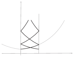
Figure 3: Constructing Floquet waves in the straight cylinder.

(see Remark 2 below) the spectral problem $\left(\ref{1.14}\right)$ in the cylindrical cell $\varpi^{0}=\omega\times\left(-\frac{1}{2},\frac{1}{2}\right)$ gets the first eigenpairs

$$\Lambda_{1}^{0}\left(\eta\right)=\left\{\begin{tabular}[c]{ll}$M_{1}+\eta^{2},$&$\eta\in\left[0,\pi\right),$\\ $M_{1}+\left(2\pi-\eta\right)^{2},$&$\eta\in\left(\pi,2\pi\right),$\end{tabular}\ \ \ \ \ \ \ \ \ \ \right.$$ (2.5)

$$U_{1}^{0}\left(y,z;\eta\right)=V_{1}\left(y\right)\left\{\begin{tabular}[c]{ll}$1,$&$\eta\in\left[0,\pi\right),$\\ $\exp\left(-2\pi iz\right),$&$\eta\in\left(\pi,2\pi\right),$\end{tabular}\ \ \ \ \ \ \ \ \ \ \right.$$ (2.6)

while, at $\eta=\pi$, the eigenvalue

$$\Lambda_{1}^{0}\left(\pi\right)=\Lambda_{2}^{0}\left(\pi\right)=M_{1}+\pi^{2}$$ (2.7)

becomes of multiplicity $2$ and has the eigenfunctions

$$U_{+}^{0}\left(y,z\right)=V_{1}\left(y\right),\text{ }U_{-}^{0}\left(y,z\right)=V_{1}\left(y\right)\exp\left(-2\pi iz\right).$$ (2.8)

It is known (see, e.g., [27, §7.6] and [21, Ch.9.10]) that a small perturbation of the cell $\varpi^{0}$ prompts perturbations of eigenvalues in $\left(\ref{1.16}\right)$. Two situations drawn in Figure 4 may occur for the first couple of eigenvalues and we shall show that a periodic singular perturbation of the cylinder $\Omega$ (see Figure 5) provides opening a gap in the continuous spectrum (as indicated by over-shadowing in Figure 4,c).

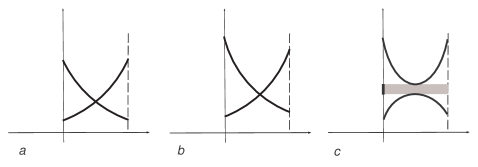
Figure 4: The perturbations (b and c) of the eigenvalue curves (a).

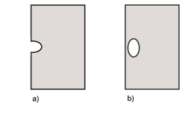
Figure 5: Singular perturbation of the periodicity cell.

2.2 The singular perturbation of the cylindrical surface.

To describe the boundary perturbation of the cylinder $\Pi^{0}=\Omega$, we introduce in a neighborhood $\Upsilon$ of the contour $\Gamma=\partial\omega$ the natural curvilinear coordinate system $\left(n,s\right)$ (Figure 6) where $n$ is the oriented distance to $\Gamma$, $n<0$ inside $\omega\cap\Upsilon$ and $s$ is the arc length on $\Gamma$ evaluated from a point $\mathcal{O}^{\prime}\in\Gamma$ counter-clockwise so that the point $\mathcal{O=}\left(\mathcal{O}^{\prime},0\right)\in\partial\Pi^{0}$ has the coordinates $n=0,$ $s=0,$ $z=0$.

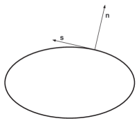
Figure 6: The curvilinear coordinates.

Given a small parameter $h$, we introduce the sets

$$\theta^{h}=\left\{x\in\Upsilon\times\mathbb{R}\mathbf{:\xi:=}h^{-1}\left(n,s,z\right)\in\theta\right\},\text{ }\varpi^{h}=\varpi^{0}\backslash\overline{\theta^{h}}$$ (2.9)

where $\theta$ is a bounded nonempty domain in the half-space $\mathbb{R}_{-}^{3}=\left\{\xi=\left(\xi_{1},\xi_{2},\xi_{3}\right):\xi_{1}<0\right\}.$ According to formula $\left(\ref{1.10}\right)$, the reference cell $\varpi^{h}$ in $\left(\ref{1.26}\right)$ generates the quasi-cylinder $\Pi^{h}$ with a singular perturbation by the $1$ - periodic family of the caves or superficial voids $\theta_{j}^{h}=\left\{x\in\Upsilon\times\mathbb{R}:h^{-1}\left(n,s,z-j\right)\in\theta\right\}$ (Figure 5,a,b).

Remark 2

We have assumed that the perturbation period $T$ is equal to $1$. If $T\neq 1$, the rescaling $x\longmapsto T^{-1}x$ turns the cylinder $\Omega$ into $\Omega_{T}=\omega_{T}\times\mathbb{R}$ while the model problem $\left(\ref{1.4}\right)$ in the new cross-section $\omega_{T}=\left\{y:Ty\in\omega\right\}$ gets the eigenvalues $T^{2}M_{k}$ where $M_{k}$ are taken from $\left(\ref{1.001}\right)$. Since $M_{1}<M_{2}$, the assumption $\left(\ref{1.21}\right)$ is satisfied in the case

$$T>\pi\left(M_{2}-M_{1}\right)^{-\frac{1}{2}}.$$ (2.10)

2.3 The boundary layer phenomenon.

To examine the behavior of eigenfunctions in the periodicity cell $\varpi^{h}$ near the boundary perturbation, we need to construct the boundary layer (see, e.g., [32], [21, Ch. 2.9]). To this end, we use the stretched coordinates $\xi$ in $\left(\ref{1.26}\right)$. Since the Laplacian $\Delta_{x}$ in the curvilinear coordinates reads

$$\Delta_{x}=\left(1+n\varkappa\left(s\right)\right)^{-1}\left(\frac{\partial}{\partial n}\left(1+n\varkappa\left(s\right)\right)\frac{\partial}{\partial n}+\frac{\partial}{\partial s}\left(1+n\varkappa\left(s\right)\right)^{-1}\frac{\partial}{\partial s}\right)+\frac{\partial^{2}}{\partial z^{2}},$$ (2.11)

where $\varkappa\left(s\right)$ is the curvature of $\Gamma$ at the point $s$, we formally have

$$\Delta_{x}\sim h^{-2}\Delta_{\xi}+h^{-1}\left(\varkappa\left(\mathcal{O}^{\prime}\right)\frac{\partial}{\partial\xi_{1}}-2\varkappa\left(\mathcal{O}^{\prime}\right)\xi_{1}\frac{\partial^{2}}{\partial\xi_{2}^{2}}\right)+...$$ (2.12)

Hence, in view of formulae (2.9), the coordinate dilation $x\longmapsto\xi$ leads to the following limit problem

$$-\Delta_{\xi}w\left(\xi\right)=0,\text{ }\xi\in\Theta\text{, }w\left(\xi\right)=g\left(\xi\right),\text{ }\xi\in\partial\Theta,$$ (2.13)

in the imperfect half-space (Figure 7,a,b)

$$\Theta=\mathbb{R}_{-}^{3}\backslash\overline{\theta}.$$ (2.14)

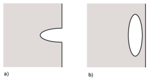
Figure 7: The rescaled perturbation of the boundary.

It is known that, for a sufficiently smooth datum $g$ with a compact support, problem $\left(\ref{1.30}\right)$ has a unique solution with a finite Dirichlet integral. In the sequel we need such the decaying solution $W\left(\xi\right)$ with the special right-hand side $g\left(\xi\right)=-\xi_{1}$ which vanishes on $\partial\Theta\backslash\partial\theta$ and obeys the asymptotic form

$$W\left(\xi\right)=-\frac{1}{2\pi}P_{\theta}\frac{\xi_{1}}{\left|\xi\right|^{3}}+O\left(\left|\xi\right|^{-3}\right),\text{ }\left|\xi\right|>R,$$ (2.15)

where $R>0$ is fixed such that $\left|x\right|<R$ for $x\in\overline{\theta}.$

Note that $-\left(2\pi\left|\xi\right|^{3}\right)^{-1}\xi_{1}$ implies the Poisson kernel and $P_{\theta}>0$ by virtue of the maximum principle.

Remark 3

The exterior Dirichlet problem for the symmetrized set $\theta^{\bullet\bullet}=\left\{\xi:\left(-\left|\xi_{1}\right|,\xi_{2},\xi_{3}\right)\in\overline{\theta}\right\}$ (cf. Figures 7 and 8) has an intrinsic integral characteristics, the polarization matrix (see [29, Appendix G]), which is extracted from asymptotics at the infinity of the harmonics $W_{j}$ under the Dirichlet conditions $W_{j}\left(\xi\right)=-\xi_{j},$ $\xi\in\partial\theta^{\bullet\bullet}$. The odd extension of $W$ from $\Theta$ onto $\mathbb{R}^{3}\backslash\theta^{\bullet\bullet}$ coincides with $W_{3}$ and, therefore, $P_{\theta}$ is proportional to an entry in the polarization tensor of $\theta^{\bullet\bullet}$. We call $P_{\theta}$ the polarization coefficient of the cavity or void $\theta$ in the half-space.

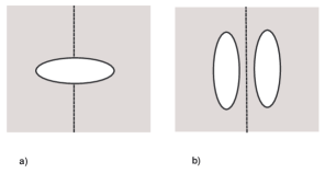
Figure 8: The symmetrization of the boundary perturbation.

2.4 The main result on asymptotics.

To identify the gap, we need two assertions on eigenvalues and eigenfunctions of the auxiliary problem

$$\left(\left(\nabla_{x}+i\eta e_{3}\right)U^{h},\left(\nabla_{x}+i\eta e_{3}\right)V\right)_{\varpi^{h}}=\Lambda^{h}\left(U^{h},V\right)_{\varpi^{h}},\text{ }V\in\mathring{H}_{per}^{1}\left(\varpi^{h};\gamma^{h}\right),$$ (2.16)

in the perturbed periodicity cell $\varpi^{h}$ in $\left(\ref{1.26}\right)$ with the lateral side $\gamma^{h}=\left\{x\in\partial\varpi^{h}:\left|z\right|<1/2\right\}.$ We enumerate the eigenvalues in the same way as in $\left(\ref{1.16}\right)$:

$$0<\Lambda_{1}^{h}\left(\eta\right)\leq\Lambda_{2}^{h}\left(\eta\right)\leq...\leq\Lambda_{p}^{h}\left(\eta\right)\leq...\rightarrow+\infty.$$ (2.17)

However, under the assumption $\left(\ref{1.21}\right)$ the first couple of eigenvalues in $\left(\ref{1.37}\right)$ is denoted by $\Lambda_{\pm}^{h}\left(\eta\right)$ while, according to $\left(\ref{1.22}\right)$, we have $\Lambda_{\pm}^{0}=M_{1}+\left(\eta-\pi\pm\pi\right)^{2}$ in the limit ($h=0$) problem $\left(\ref{1.14}\right)$ in $\varpi=\varpi^{0}$ and the corresponding eigenfunctions are given by $\left(\ref{1.23}\right).$

Theorem 4

There exist positive numbers $h_{0},\beta_{0},c_{0}$ such that, for any $h\in\left(0,h_{0}\right]$ and $\left|\beta\right|\leq\beta_{0}h^{-\frac{5}{4}}$, the first couple of eigenvalues in $\left(\ref{1.37}\right)$ of the problem $\left(\ref{1.36}\right)$ on the periodicity cell $\varpi^{h}$, determined in $\left(\ref{1.26}\right)$, takes the asymptotic form

$$\Lambda_{\pm}^{h}\left(\pi+\beta h^{3}\right)=M_{1}+\pi^{2}+h^{3}\left(\mathcal{P\pm}\sqrt{\mathcal{P}^{2}+4\pi^{2}\beta^{2}}\right)+\widetilde{\Lambda}_{\pm}^{h}\left(\pi+\beta h^{3}\right)$$ (2.18)

where the remainder admits the estimate

$$\left|\widetilde{\Lambda}_{\pm}^{h}\left(\pi+\beta h^{3}\right)\right|\leq C_{\Lambda}h^{\frac{7}{2}}$$ (2.19)

and the positive quantity

$$\mathcal{P=}P_{\theta}\left|\partial_{n}V_{1}\left(\mathcal{O}^{\prime}\right)\right|^{2}$$ (2.20)

is calculated according to $\left(\ref{1.32}\right)$ and $\left(\ref{1.000}\right)$.

The asymptotic formula $\left(\ref{1.33}\right)$, $\left(\ref{1.35}\right)$ will be derived in §3 and the remainder estimate $\left(\ref{1.34}\right)$ in §4. To detect a gap in the continuous spectrum of the problem $\left(\ref{1.11}\right)$ in the quasi-cylinder $\Pi^{h}$, we also prove the following intelligible inequalities.

Lemma 5

Entries of the eigenvalue sequences $\left(\ref{1.37}\right)$ and $\left(\ref{1.16}\right)$ of the auxiliary problems in the cells $\varpi^{h}$ and $\varpi^{0}$, respectively, are in the relationship

$$\Lambda_{p}^{0}\left(\eta\right)\leq\Lambda_{p}^{h}\left(\eta\right)\leq\Lambda_{p}^{0}\left(\eta\right)+C_{p}h^{3},$$ (2.21)

where $C_{p}$ is independent of $\eta\in\left[0,2\pi\right)$ and $h\in\left(0,h_{0}\right].$

Proof. Let $\mathcal{A}_{\eta}^{h}$ be a unbounded operator in $L^{2}\left(\varpi^{h}\right)$ generated by the closed positive Hermitian form $Q_{\eta}\left(\cdot,\cdot,\varpi^{h}\right)$ on the left of $\left(\ref{1.14}\right)$ (cf. [3, §10.2]). We employ the max-min principle (see [3, Thm. 10.2.2])

$$\Lambda_{p}^{h}\left(\eta\right)=\underset{\mathcal{E}_{p}}{\max}\underset{U\in\mathcal{E}_{p}\backslash\left\{0\right\}}{\inf}\frac{Q_{\eta}\left(U,U;\varpi^{h}\right)}{\left\|U;L^{2}\left(\varpi^{h}\right)\right\|^{2}},\text{ }p\in\mathbf{\mathbb{N}.}$$ (2.22)

Here $\mathcal{E}_{p}$ is any subspace in $\mathring{H}_{per}^{1}\left(\varpi^{h};\gamma^{h}\right)$ of co-dimension $p-1$, in particular, $\mathcal{E}_{1}=\mathring{H}_{per}^{1}\left(\varpi^{h};\gamma^{h}\right).$

Let the eigenfunctions $U_{p}^{0}\left(\cdot,\eta\right)$ corresponding to $\Lambda_{p}^{0}\left(\eta\right)$ satisfy the normalization and orthogonality conditions

$$\left(U_{p}^{0},U_{q}^{0}\right)_{\varpi^{0}}=\delta_{p,q},\text{ }p,q\in\mathbf{\mathbb{N}},$$ (2.23)

where $\delta_{p,q}$ stands for Kronecker’s symbol. The subspace $\mathfrak{I}_{p}\subset\mathring{H}_{per}^{1}\left(\varpi^{h};\gamma^{h}\right)$ is spanned over the functions $X_{h}U_{1}^{0},...,X_{h}U_{p}^{0}$ while $X_{h}\in C_{per}^{\infty}\left(\overline{\varpi^{0}}\right)$ is such that

$$X_{h}\left(x\right) =0\text{ \ for \ }\left|x-\mathcal{O}\right|\leq C_{X}h,X_{h}\left(x\right)=1\text{ \ for \ }\left|x-\mathcal{O}\right|\geq 2c_{X}h,$$ (2.24)

$$X_{h}\left(x\right) =0\text{ \ for \ }x\in\theta^{h},\ 0\leq X_{h}\leq 1,\ \left|\nabla_{x}X_{h}\left(x\right)\right|\leq ch^{-1}.\$$

In other words, $X_{h}$ is equal to $1$ everywhere in $\varpi^{h}$, except in the vicinity of $\mathcal{O}$, and $X_{h}$ vanishes in the cavern. We have

$$\left(X_{h}U^{p},X_{h}U^{q}\right)_{\varpi^{h}} =\left(U^{p},U^{q}\right)_{\varpi^{0}}+\left(\left(1-X_{h}^{2}\right)U^{p},U^{q}\right)_{\varpi^{0}}\geq\delta_{p,q}-c_{pq}h^{2}h^{3},$$ (2.25)

$$Q_{\eta}\left(U^{p},U^{q};\varpi^{h}\right) \leq Q_{\eta}\left(U^{p},U^{q};\varpi^{0}\right)+c_{pq}\left(\left\|U^{p};H^{1}\left(\Xi_{h}\right)\right\|+h^{-1}\left\|U^{p};L^{2}\left(\Xi_{h}\right)\right\|\right)\cdot$$

$$\ \ \ \ \ \ \ \ \ \ \ \ \ \ \ \ \ \ \cdot\left(\left\|U^{q};H^{1}\left(\Xi_{h}\right)\right\|+h^{-1}\left\|U^{p};L^{2}\left(\Xi_{h}\right)\right\|\right)$$

$$\leq\Lambda_{p}^{0}\delta_{p,q}+c_{pq}\left(h^{3}+h^{-2}h^{2}h^{3}\right).$$

Here come the factors $h^{-1}$ and $h^{2}$ from the differentiation of $X_{h}$ and the formula

$$\left|U^{p}\left(x\right)\right|^{2}\leq c_{p}\left|x-\mathcal{O}\right|^{2}\leq C_{p}h^{2},\text{ }x\in\Xi_{h},$$

while $h^{3}$ is order of the volume of the set $\Xi_{h}=$ supp$\left(1-X_{h}\right)\supset$ supp$\left|\nabla_{x}X_{h}\right|.$

The intersection of the subspaces $\mathcal{E}_{p}$ and $\mathfrak{I}_{p}$ contains the nontrivial linear combination

$$\mathcal{U}_{p}=X_{h}{\displaystyle\sum\limits_{j=1}^{p}}a_{p}U^{p},{\displaystyle\sum\limits_{j=1}^{p}}\left|a_{p}\right|^{2}=1.$$ (2.26)

Hence, according to $\left(\ref{1.40}\right)$ and $\left(\ref{1.42}\right)$, we derive that

$$\Lambda_{p}^{h}\left(\eta\right)\leq\underset{\mathcal{E}_{p}}{\max}\frac{Q_{\eta}\left(\mathcal{U}_{p};\varpi^{h}\right)}{\left\|\mathcal{U}_{p};L^{2}\left(\varpi^{h}\right)\right\|^{2}}\leq\frac{{\displaystyle\sum\limits_{j=1}^{p}}\Lambda_{j}^{0}\left(\eta\right)+C_{p}h^{3}}{1-C_{p}h^{3}}$$

and the right inequality in $\left(\ref{1.39}\right)$ is proved.

The left inequality can be easily derived by applying the max-min principle to the operator $\mathcal{A}_{\eta}^{0}$ and extending eigenfunctions $U_{p}^{h}$ by zero from $\varpi^{h}$ onto $\varpi^{0}.$

2.5 Detecting the gap.

By Lemma 5 and formula $\left(\ref{1.200}\right)$, we conclude that

$$\Lambda_{1}^{h}\left(\eta\right) \leq M_{1}+\min\left\{\eta^{2},\left(2\pi-\eta\right)^{2}\right\}+C_{1}h^{3},$$ (2.27)

$$\Lambda_{2}^{h}\left(\eta\right) \geq\min\left\{M_{1}+\max\left\{\eta^{2},\left(2\pi-\eta\right)^{2}\right\},\ M_{2}+\min\left\{\eta^{2},\left(2\pi-\eta\right)^{2}\right\}\right\}.$$

Hence, in view of the assumption $\left(\ref{1.21}\right)$ we can choose $\eta_{0}>\left(2\pi\right)^{-1}\max\left\{C_{1},3\mathcal{P}\right\}$ and $h_{0}>0$ such that, for $h\in\left(0,h_{0}\right]$ and $\eta\in\left[0,\pi-\eta_{0}h^{3}\right)\cup\left(\pi+\eta_{0}h^{3},2\pi\right)$, the interval

$$\left(M_{1}+\pi^{2},M_{1}+\pi^{2}+2\mathcal{P}h^{3}\right)$$

is free of eigenvalues $\left(\ref{1.37}\right)$. In the case $\left|\eta-\pi\right|\leq\eta_{0}h^{3}$ we apply Theorem 4 to observe that also the interval

$$\left(M_{1}+\pi^{2}+C_{\Lambda}h^{\frac{7}{2}},M_{1}+\pi^{2}+2\mathcal{P}h^{3}-C_{\Lambda}h^{\frac{7}{2}}\right)$$ (2.28)

does not contain the eigenvalues. We emphasize that the endpoints in $\left(\ref{1.45}\right)$ are established by the following inequalities taken from Theorem 4:

$$\Lambda_{1}^{h}\left(\eta\right) \leq M_{1}+\pi^{2}h^{3}\left(\mathcal{P-P}\sqrt{1+4\pi^{2}\mathcal{P}^{-2}\eta_{0}^{2}}\right)+C_{\Lambda}h^{\frac{7}{2}}\leq M_{1}+\pi^{2}+C_{\Lambda}h^{\frac{7}{2}},$$

$$\Lambda_{2}^{h}\left(\eta\right) \geq M_{1}+\pi^{2}h^{3}\left(\mathcal{P+P}\sqrt{1+4\pi^{2}\mathcal{P}^{-2}\eta_{0}^{2}}\right)-C_{\Lambda}h^{\frac{7}{2}}\geq M_{1}+\pi^{2}+2\mathcal{P}h^{3}-C_{\Lambda}h^{\frac{7}{2}}.$$

These two facts provide the main result in the paper.

Theorem 6

Under the assumption $\left(\ref{1.21}\right)$, there exist positive numbers $h_{0}$ and $c_{0}$ such that, for $h\in\left(0,h_{0}\right]$, the essential spectrum $\left(\ref{1.12}\right)$ of the problem $\left(\ref{1.11}\right)$ in the periodic waveguide $\Pi^{h}$ with the periodicity cell $\varpi^{h}$ in $\left(\ref{1.26}\right)$ has a gap of length $l\left(h\right)$,

$$\left|l\left(h\right)-2\mathcal{P}h^{3}\right|\leq c_{0}h^{\frac{7}{2}},$$ (2.29)

situated just after the first segment $\Upsilon_{1}^{h}$ in $\left(\ref{1.12}\right)$. Here $\mathcal{P}$ is the positive quantity $\left(\ref{1.35}\right)$.

We finally mention that under the assumption $M_{1}+\pi^{2}>M_{2}$ opposite to $\left(\ref{1.21}\right),$ the first and second segment $\Upsilon_{1}^{h}$ and $\Upsilon_{2}^{h}$ intersect (cf. Figure 9 where two dotted curves correspond to $\left(\ref{1.200}\right)$ with $p=2$ and $q=0,1$) and therefore, the gap discovered in Theorem 6 does not occur. This conclusion readily follows from the rough estimate $\left(\ref{1.39}\right)$ for the perturbated eigenvalue $M_{2}+\min\left\{\eta^{2},\left(2\pi-\eta\right)^{2}\right\}$ in the auxiliary problem in $\varpi^{h}$.

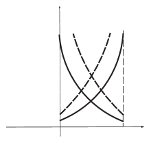
Figure 9: Overlapping of the bands.

If $M_{2}=M_{1}+\pi^{2}$, then the gap is still open because $\Lambda_{2}^{h}\left(0\right)>M_{2}$ and Theorem 4 is still valid. At the same time, the gap length is $O\left(h^{3}\right)$ only in the case when $M_{2}$ is simple and $\partial_{n}V_{2}\left(\mathcal{O}^{\prime}\right)\neq 0$, but $l\left(h\right)=o\left(h^{3}\right)$ provide the normal derivative of an eigenfunction corresponding to $M_{2}$ vanishes at the point $\mathcal{O}^{\prime}$. This conclusion can be confirmed by an asymptotic analysis of eigenvalues, similar to §3 and §4. However, calculations become much more combersome and we omit them here while refereing to [21, Ch. 9,10] for general asymptotic procedures.

3 The asymptotic analysis

3.1 The asymptotic ansätze

Let us examine the eigenvalues $\Lambda_{\pm}^{h}\left(\eta\right)$ of the spectral problem $\left(\ref{1.14}\right)$ in the perturbed periodicity cell $\varpi^{h}$ which are close to the double eigenvalue $\left(\ref{1.24}\right)$ of the problem in $\varpi^{0}$. We fix the dual variable of the Gel’fand transform

$$\eta=\pi+\beta h^{3},$$ (3.1)

where $\beta\in\mathbb{R}$ is the deviation parameter. By varying $\beta$, we watch over the eigenvalues $\Lambda_{\pm}^{h}\left(\eta\right)$ in the vicinity of the collision point in Figure 4,a. Note that the factor $h^{3}$ is adjusted with the second term in the eigenvalue asymptotic ansätze [24] (see also [21, Ch. 9] and [26])

$$\Lambda_{\pm}^{h}\left(\eta\right)=\Lambda^{0}+h^{3}\Lambda_{\pm}^{{}^{\prime}}\left(\beta\right)+\widetilde{\Lambda}_{\pm}^{h}\left(\eta\right).$$ (3.2)

Here $\Lambda^{0}=M_{1}+\pi^{2},$ $\Lambda_{\pm}^{{}^{\prime}}\left(\beta\right)$ is a correction term to be found out and $\widetilde{\Lambda}_{\pm}^{h}\left(\eta\right)$ a small remainder to be estimated in §4. The asymptotic ansätze for the corresponding eigenfunctions looks as follows:

$$U_{\pm}^{h}\left(x;\eta\right)=U_{\pm}^{0}\left(x;\beta\right)+h\chi\left(x\right)\left(w_{\pm}^{1}\left(\xi;\beta\right)+hw_{\pm}^{2}\left(\xi;\beta\right)\right)+h^{3}U_{\pm}^{\prime}\left(x;\beta\right)+\widetilde{U}_{\pm}^{h}\left(x;\eta\right).$$ (3.3)

The main term

$$U_{\sigma}^{0}\left(x;\beta\right)=a_{+}^{\sigma}\left(\beta\right)U_{+}\left(x\right)+a_{-}^{\sigma}\left(\beta\right)U_{-}\left(x\right),\text{ }\sigma=+,-,$$ (3.4)

is a linear combination of functions $\left(\ref{1.25}\right)$ with the coefficient column $a^{\sigma}=\left(a_{+}^{\sigma},a_{-}^{\sigma}\right)^{\top}$ while $\left|a^{\sigma}\right|=1$ and $\top$ stands for transposition. The boundary layer terms $w_{\sigma}^{q}$ are intended to compensate for a discrepancy produced in the Dirichlet condition on the surface $\partial\theta^{h}\cap\partial\varpi^{h}$ by the term $U_{\pm}^{0}$. Since $w_{\sigma}\left(\xi;\beta\right)$ is defined only in the set $\mathcal{U\cap\varpi}^{h}$, the cut-off function $\chi$ is introduced in $\left(\ref{2.3}\right)$ such that $\chi=0$ outside a neighborhood of $\mathcal{O}$ and $\chi=1$ in the vicinity of the point $\mathcal{O}$. The correction term $U_{\sigma}^{\prime}$ is used to compensate for discrepancy of $U_{\sigma}^{0}$ and $h\chi w_{\sigma}^{1}$ in the equation with the differential operator

$$\Delta_{y}+\left(\partial_{z}+i\eta\right)^{2}+\Lambda_{\sigma}^{h}\left(\eta\right) \sim\Delta_{y}+\left(\partial_{z}+i\pi\right)^{2}+\Lambda^{0}+h^{3}\left(2i\beta\left(\partial_{z}+i\pi\right)+\Lambda_{\sigma}^{{}^{\prime}}\left(\beta\right)\right)+...$$ (3.5)

$$=:L^{0}\left(\nabla_{x}\right)+h^{3}L^{\prime}\left(\nabla_{x};\beta\right)+...$$

which is decomposed in accordance with $\left(\ref{2.1}\right)$ and $\left(\ref{2.2}\right).$ Notice that the second boundary layer term $h\chi w_{\pm}^{2}$ is linear in $\varkappa\left(\mathcal{O}^{\prime}\right)$ (cf. $\left(\ref{1.29}\right)$), however it does not influences $\Lambda_{\pm}^{{}^{\prime}}\left(\beta\right)$ in $\left(\ref{2.2}\right)$ and becomes important only in §4 for justification estimates (see Section 3.4). This observation displays the effect of opening the gap to be independent of the curvature $\varkappa$ of the contour $\partial\omega.$

The function $U_{\pm}^{{}^{\prime}}$ in $\left(\ref{2.4}\right)$ gets a singularity at the point $\mathcal{O}$ and, hence, we ought to introduce another cut-off function $X_{h}$ into $\left(\ref{2.3}\right)$ (see $\left(\ref{4.8}\right)$). However, since the asymptotic analysis in this section is formal, we avoid to multiply $U_{\pm}^{{}^{\prime}}$ with $X_{h}$ here. To accept this mathematical licence, one can assume that the coordinate origin $\xi=0$ lies inside $\theta$, i.e. $\mathcal{O\notin}\overline{\mathcal{\varpi}^{h}}$ for any $h\in\left(0,h_{0}\right].$

3.2 Calculating the asymptotic terms

Since the eigenfunction $V_{1}$ of the problem $\left(\ref{1.4}\right)$ is smooth near the boundary $\partial\omega$, the Taylor formula and the Dirichlet condition yield

$$U_{\sigma}^{0}\left(x;\beta\right)=\left(a_{+}^{\sigma}\left(\beta\right)+a_{-}^{\sigma}\left(\beta\right)\right)n\partial_{n}V_{1}\left(\mathcal{O}^{\prime}\right)+{\displaystyle\sum\limits_{\pm}}a_{\pm}^{\sigma}\left(\beta\right)\mathbf{U}^{\pm}\left(n,s,z\right)+O\left(\left|n\right|^{3}+\left|s\right|^{3}\right)=$$ (3.6)

$$=h\left(a_{+}^{\sigma}\left(\beta\right)+a_{-}^{\sigma}\left(\beta\right)\right)\xi_{1}\partial_{n}V\left(\mathcal{O}^{\prime}\right)+h^{2}{\displaystyle\sum\limits_{\pm}}a_{\pm}^{\sigma}\left(\beta\right)\mathbf{U}^{\pm}\left(\xi\right)+O\left(h^{3}\right),\text{ }$$

$$\ \ \ \ \ \ \ \ \ \ \ \ \ \ \ \ \ \ \ \ \ \ \ \ \ \ \ \ \ \ \ \ \ \ \ \ \ \ \ \ \ \ \ \ \ \ \ \ \ \ \ \ \ \ \ \ \ \ \ \ \ \ \ \ \ \ \ \ \ \ \ \ \ \ \ \ \ \ \ \ \ \ \ \ \ \ \ \ \ \ \ \ \ \ \ \ \ \ \ \ \ x\in\partial\theta^{h}\cap\partial\varpi^{h},$$

$$\mathbf{U}^{\pm}\left(\xi\right)=\frac{\xi_{1}^{2}}{2}\partial_{n}^{2}V_{1}\left(\mathcal{O}^{\prime}\right)+\xi_{1}\xi_{2}\partial_{s}\partial_{n}V_{1}\left(\mathcal{O}^{\prime}\right)-2\pi i\delta_{\pm,-}\xi_{1}\xi_{3}\partial_{n}V_{1}\left(\mathcal{O}^{\prime}\right).$$ (3.7)

Here we used the definitions of $U_{\sigma}^{0}$ and $\xi$ in $\left(\ref{2.4}\right)$ and $\left(\ref{1.25}\right)$. Recalling the special solution $W$ of the limit problem $\left(\ref{1.30}\right)$ with $g\left(\xi\right)=-\xi_{1}$, we set

$$w_{\sigma}^{1}\left(\xi\right)=\left(a_{+}^{\sigma}\left(\beta\right)+a_{-}^{\sigma}\left(\beta\right)\right)\partial_{n}V_{1}\left(\mathcal{O}^{\prime}\right)W\left(\xi\right)$$ (3.8)

in order to compensate for the main discrepancy $O\left(h\right)$ in $\left(\ref{2.6}\right)$. By the asymptotic expansion $\left(\ref{1.32}\right)$ we obtain

$$hw_{\sigma}^{1}\left(\xi\right)=-hA_{\sigma}\left(\beta\right)\frac{\xi_{1}}{2\pi\left|\xi\right|^{3}}+O\left(\frac{h}{\left|\xi\right|^{3}}\right)=-h^{3}A_{\sigma}\left(\beta\right)\frac{n}{2\pi r^{3}}+O\left(\frac{h^{4}}{r^{3}}\right)$$ (3.9)

where $r=\sqrt{n^{2}+s^{2}+z^{2}}=h\left|\xi\right|$ and

$$A_{\sigma}\left(\beta\right)=\left(a_{+}^{\sigma}\left(\beta\right)+a_{-}^{\sigma}\left(\beta\right)\right)\partial_{n}V_{1}\left(\mathcal{O}^{\prime}\right)P_{\theta}.$$ (3.10)

After applying the differential operator $\left(\ref{2.5}\right)$ to the right-hand side of $\left(\ref{2.3}\right)$ we collect coefficients on $h^{3}$ and derive the differential equation

$$L^{0}\left(\nabla_{x}\right)U_{\sigma}^{{}^{\prime}}\left(x;\beta\right) =F_{\sigma}^{\prime}\left(x;\beta\right):=$$ (3.11)

$$:=-L^{\prime}\left(\nabla_{x};\beta\right)U_{\sigma}^{{}^{\prime}}\left(x;\beta\right)+L^{0}\left(\nabla_{x}\right)\left(\chi\left(x\right)A_{\sigma}\left(\beta\right)\frac{n}{2\pi r^{3}}\right),\text{ }x\in\varpi^{0},$$

which is to be supplied with the following Dirichlet condition on the lateral side $\gamma^{0}$ of the cylindrical cell $\varpi^{0}:$

$$U_{\sigma}^{{}^{\prime}}\left(x;\beta\right)=0,\text{ }x\in\gamma^{0}.$$ (3.12)

The first term $L^{\prime}U_{\sigma}^{0}$ on the right of $\left(\ref{2.10}\right)$ is smooth in $\overline{\varpi^{0}}$ but the second one gets a singularity at the point $\mathcal{O}\in\gamma^{0}$. By means of $\left(\ref{1.28}\right)$ (see also $\left(\ref{1.29}\right)$ and $\left(\ref{2.5}\right)$) we conclude the representation

$$L^{0}\left(\nabla_{x}\right)=\frac{\partial^{2}}{\partial n^{2}}+\frac{\partial^{2}}{\partial s^{2}}+\frac{\partial^{2}}{\partial z^{2}}-2n\varkappa\left(s\right)\frac{\partial^{2}}{\partial s^{2}}+\mathcal{L}^{0}\left(x,\nabla_{x}\right)$$ (3.13)

where $\mathcal{L}^{0}$ is a first-order differential operator. Hence,

$$L^{0}\left(\nabla_{x}\right)\left(\chi\left(x\right)r^{-3}n\right)=O\left(r^{-3}\right),\text{ }r\rightarrow+0.$$ (3.14)

The strong singularity $\left(\ref{2.13}\right)$ of the right-hand side does not allow for a solution $U_{\sigma}^{\prime}$ of problem $\left(\ref{2.10}\right),$ $\left(\ref{2.11}\right)$ in the Sobolev space $\mathring{H}^{1}\left(\varpi^{0};\gamma^{0}\right).$

3.3 The regular correction term for the eigenfunctions.

Let us move into the scale of Kondratiev spaces $V_{\tau}^{l}\left(\varpi^{0}\right)$ (see [18] and, e.g., [19, 20]) equipped with the weighted norm

$$\left\|U;V_{\tau}^{l}\left(\varpi^{0}\right)\right\|=\left(\sum_{k=0}^{l}\left\|\rho^{\tau-l-k}\nabla_{x}^{k}U;L^{2}\left(\varpi^{0}\right)\right\|^{2}\right)^{\frac{1}{2}}$$ (3.15)

where $\rho\left(x\right)=$dist$\left(x,\mathcal{O}\right)$, $\nabla_{x}^{k}U$ is the family of all order $k$ derivatives of $U$ while $l\in\left\{0,1,..\right\}$ and $\tau\in\mathbf{\mathbb{R}}$ are the smoothness and weight indices, respectively. By the one-dimensional Hardy inequality with the particular exponent $\alpha=1,$

$${\displaystyle\int\limits_{0}^{+\infty}}\rho^{\alpha-1}\left|u\left(\rho\right)\right|^{2}d\rho\leq\frac{4}{\alpha^{2}}{\displaystyle\int\limits_{0}^{+\infty}}\rho^{\alpha+1}\left|\frac{du}{d\rho}\left(\rho\right)\right|^{2}d\rho,\text{ }\alpha>0\text{, }u\in C_{c}^{1}\left[0,+\infty\right),$$ (3.16)

we obtain that

$$\left\|\rho^{-1}U;L^{2}\left(\varpi^{0}\right)\right\|^{2}\leq c\left\|U;H^{1}\left(\varpi^{0}\right)\right\|^{2}.$$ (3.17)

Thus, the space

$$\mathring{V}_{0,per}^{1}\left(\varpi^{0},\gamma^{0}\right)=\left\{U\in V_{0}^{1}\left(\varpi^{0}\right):U=0\text{ on }\gamma^{0},\text{ }U\text{ is }1-\text{periodic in }z\right\}$$

coincides with the space $\mathring{H}_{per}^{1}\left(\varpi^{0},\gamma^{0}\right)$ algebraically and topologically. This means that the mapping

$$\mathring{V}_{0,per}^{1}\left(\varpi^{0},\gamma^{0}\right)\rightarrow\mathring{V}_{0,per}^{1}\left(\varpi^{0},\gamma^{0}\right)^{\ast},$$ (3.18)

associated with the problem $\left(\ref{2.10}\right)$, $\left(\ref{2.11}\right)$, inherits all properties of the mapping

$$\mathring{H}_{per}^{1}\left(\varpi^{0},\gamma^{0}\right)\rightarrow\mathring{H}_{per}^{1}\left(\varpi^{0},\gamma^{0}\right)^{\ast}.$$ (3.19)

Moreover, theorems in [18] on lifting smoothness and shifting the weight indices (see also [19, Theorems 4.1.2 and 4.2.1]) convey these properties to the mapping

$$\mathring{V}_{\tau,per}^{1}\left(\varpi^{0},\gamma^{0}\right)\cap V_{l+\tau,per}^{l+1}\left(\varpi^{0}\right)\rightarrow V_{l+\tau,per}^{l-1}\left(\varpi^{0}\right)$$ (3.20)

in the case

$$l\in\mathbf{\mathbb{N}}\text{, }\tau\in\left(-\frac{3}{2},\frac{3}{2}\right).$$ (3.21)

Remark 7

The bound $\pm\frac{3}{2}$ for the weight index $\tau$ in $\left(\ref{2.30}\right)$ may be computed as follows: the ”linear” function $x\longmapsto\chi\left(x\right)n$ belongs to $V_{l+\tau}^{l+1}\left(\varpi^{0}\right)$ under the restriction $\tau>-\frac{3}{2}$ while the Poisson kernel $\chi\left(x\right)nr^{-3}$ lives outside $V_{l+\tau}^{l+1}\left(\varpi^{0}\right)$ in the case $\tau<\frac{3}{2}$. An explanation of such a mnemonic rule, maintained by the general theory, can be found in the introductory chapters of books [19, 20].

Taking into account the singularity of $F_{\sigma}^{\prime}$ at the point $\mathcal{O},$ we see that

$$F_{\sigma}^{\prime}\in V_{l+\tau,per}^{l-1}\left(\varpi^{0}\right)\text{ for any }\tau\in\left(\frac{1}{2},\frac{3}{2}\right).$$

Recall that $\Lambda^{0}=M_{1}+\pi^{2}$ is a double eigenvalue of problem $\left(\ref{1.14}\right)$ in the cylindrical cell $\varpi^{0}$ (see $\left(\ref{1.24}\right)$ and $\left(\ref{1.25}\right)$). Thus, the co-kernel of the mapping $\left(\ref{2.19}\right)$ is spanned over the functions $U_{\pm}$ and the problem $\left(\ref{2.10}\right)$, $\left(\ref{2.11}\right)$ admits a solution in $V_{l+\tau,per}^{l+1}\left(\varpi^{0}\right)$ with $\tau\in\left(\frac{1}{2},\frac{3}{2}\right)$ if and only if

$${\displaystyle\int\nolimits_{\varpi^{0}}}\overline{U_{\pm}\left(x\right)}F_{\sigma}^{\prime}\left(x;\beta\right)dx=0.$$ (3.22)

Note that $U_{\pm}\left(x\right)=O\left(\left|n\right|\right)$ in $\Upsilon\times\left(-\frac{1}{2},\frac{1}{2}\right)$ and, in view of $\left(\ref{2.13}\right)$, the integral in $\left(\ref{2.31}\right)$ is convergent.

Let the compatibility conditions $\left(\ref{2.31}\right)$ be satisfied. The orthogonality conditions

$${\displaystyle\int\nolimits_{\varpi^{0}}}\overline{U_{\pm}\left(x\right)}U_{\sigma}^{\prime}\left(x;\beta\right)dx=0$$ (3.23)

make the solution unique.

Remark 8

. The general results [18, 23], (see also [19, Ch.2.3]) furnish an asymptotic form of the solution $U_{\sigma}^{\prime}.$ By $\left(\ref{1.28}\right)$, $\left(\ref{1.29}\right)$ and $\left(\ref{2.5}\right)$, $\left(\ref{2.10}\right)$, we have

$$F_{\sigma}^{\prime}\left(x;\beta\right)=r^{-5}Q_{F}\left(n,s,z\right)+O\left(r^{-2}\right)\text{, }r\rightarrow 0^{+}\text{,}$$ (3.24)

where $Q_{...}$ stands for a homogeneous polynomial of degree 2. A routine and traditional calculation brings the expansion

$$U_{\sigma}^{\prime}\left(x;\beta\right)=r^{-3}Q_{U}\left(n,s,z\right)+O\left(r^{0}\right)\text{, }r\rightarrow 0^{+}\text{,}$$ (3.25)

which as well as $\left(\ref{33.1}\right)$ can be differentiated under the convention $\nabla_{x}O\left(r^{t}\right)=O\left(r^{t-1}\right)$. We need not explicit formulas for $Q_{F}$ and $Q_{U}$, however the estimate

$$\nabla_{x}^{k}U_{\sigma}^{\prime}\left(x;\beta\right)\leq c_{k}\left(1+\left|\beta\right|\right)r^{-1-k},\text{ }k=0,1...,$$ (3.26)

inherited from $\left(\ref{33.2}\right)$, will be useful in §4. Constants $c_{k}$ in $\left(\ref{33.3}\right)$ do not depend on the parameter $\beta$ while $Q_{F}$ and $Q_{U}$ are linear in $\beta$ (see formula for $L^{\prime}$ in $\left(\ref{2.5}\right)$).

All the above conclusions, of course, are known explicitly for the Poisson kernel.

3.4 The correction term for the eigenvalues.

Let us compute the left-hand side of $\left(\ref{2.31}\right)$. Applying formulae $\left(\ref{2.5}\right)$, $\left(\ref{1.000}\right)$ and $\left(\ref{1.25}\right)$, $\left(\ref{2.4}\right)$, we readily get

$$I_{1}={\displaystyle\int\nolimits_{\varpi^{0}}}\overline{U_{\pm}\left(x\right)}L^{\prime}\left(\nabla_{x};\beta\right)U_{\sigma}^{0}\left(x;\beta\right)dx=\ \ \ \ \ \ \ \ \ \ \ \ \ \ \ \ \ \ \ \ \ \ \ \ \ \ \ \ \ \ \ \ \ \ \ \ \ \ \ \ \ \ \ \$$ (3.27)

$$={\displaystyle\int\nolimits_{\omega}}\left|V\left(y\right)\right|^{2}dy{\displaystyle\int\nolimits_{0}^{1}}\left(\overline{\exp\left(\left(-\pi\pm\pi\right)iz\right)}\left(a_{\sigma}^{+}\left(\beta\right)\left(-2\pi\beta+\Lambda_{\sigma}^{\prime}\left(\beta\right)\right)\right)\right.+$$

$$+\left.\left(a_{\sigma}^{-}\left(\beta\right)\left(2\pi\beta+\Lambda_{\sigma}^{\prime}\left(\beta\right)\right)\exp\left(-2\pi iz\right)\right)\right)dz=$$

$$=a_{\sigma}^{\pm}\left(\beta\right)\left(\mp 2\pi\beta+\Lambda_{\sigma}^{\prime}\left(\beta\right)\right).\ \ \ \ \ \ \ \ \ \ \ \ \ \ \ \ \ \ \ \ \ \ \ \ \ \ \ \ \ \ \ \ \ \ \ \ \ \ \ \ \ \ \ \ \ \$$

To calculate the second integral, we employ the method [22]. Using the Green formula in the domain $\varpi^{0}\backslash\mathcal{B}_{\delta}$ where $\mathcal{B}_{\delta}=\left\{x\in\Upsilon\times\left(-\frac{1}{2},\frac{1}{2}\right):r<\delta\right\}$ and $\delta>0$ is small, we have

$$I_{2} ={\displaystyle\int\nolimits_{\varpi^{0}}}\overline{U_{\pm}\left(x\right)}L^{0}\left(\nabla_{x}\right)\left(\chi\left(x\right)A_{\sigma}\dfrac{n}{4\pi r^{3}}\right)dx=A_{\sigma}\underset{\delta\rightarrow 0}{\lim}{\displaystyle\int\nolimits_{\varpi^{0}\backslash\mathcal{B}_{\delta}}}\overline{U_{\pm}\left(x\right)}L^{0}\left(\nabla_{x}\right)\dfrac{\chi\left(x\right)n}{4\pi r^{3}}dx=$$ (3.28)

$$=-A_{\sigma}\underset{\delta\rightarrow 0}{\lim}{\displaystyle\int\nolimits_{\partial\mathcal{B}_{\delta}\cap\varpi^{0}}}\left(\overline{U_{\pm}\left(x\right)}\dfrac{\partial}{\partial\widehat{N}}\dfrac{n}{2\pi r^{3}}-\dfrac{n}{2\pi r^{3}}\dfrac{\partial}{\partial\widehat{N}}\overline{U_{\pm}\left(x\right)}\right)ds_{x}.$$

Here $\dfrac{\partial}{\partial\widehat{N}}=\dfrac{\partial}{\partial N}+i\pi\dfrac{z}{r}$ and $N$ is the interior normal on the surface $\partial\mathcal{B}_{\delta}\cap\varpi^{0}$. Since the gradient operator in the curvilinear coordinates takes the form

$$\left(\frac{\partial}{\partial n},\left(1+n\varkappa\left(s\right)\right)^{-1}\frac{\partial}{\partial s},\frac{\partial}{\partial z}\right),$$

we obtain

$$N\left(x\right)=\left(r^{2}+s^{2}\left(\left(1+n\varkappa\left(s\right)\right)^{-2}-1\right)\right)^{-\frac{1}{2}}\left(n,\left(1+n\varkappa\left(s\right)\right)^{-1}s,z\right),$$

$$\dfrac{\partial}{\partial N}=\left(r^{2}+s^{2}\left(\left(1+n\varkappa\left(s\right)\right)^{-2}-1\right)\right)^{-\frac{1}{2}}\left(n\frac{\partial}{\partial n},\left(1+n\varkappa\left(s\right)\right)^{-2}s\frac{\partial}{\partial s},z\frac{\partial}{\partial z}\right).$$

Thus, computing the limit in $\left(\ref{2.33}\right)$, we can make the changes

$$U_{\pm}\left(x\right)\longmapsto n\partial_{n}V_{1}\left(\mathcal{O}^{\prime}\right)\text{, }\dfrac{\partial}{\partial\widehat{N}}\longmapsto\frac{\partial}{\partial r}=\frac{n}{r}\frac{\partial}{\partial n}+\frac{s}{r}\frac{\partial}{\partial s}+\frac{z}{r}\frac{\partial}{\partial z}.$$

(cf. $\left(\ref{1.25}\right)$, $\left(\ref{2.6}\right)$). Taking the relation $mes_{2}\left(\partial\mathcal{B}_{\delta}\cap\varpi^{0}\right)=2\pi\delta^{2}+O\left(\delta^{3}\right)$ into account, we then arrive at the formula

$$I_{2} =-A_{\sigma}\left(\beta\right)\partial_{n}V_{1}\left(\mathcal{O}^{\prime}\right)\underset{\delta\rightarrow 0}{\lim}{\displaystyle\int\nolimits_{\partial\mathcal{B}_{\delta}\cap\varpi^{0}}}\left(n\dfrac{\partial}{\partial r}\dfrac{n}{2\pi r^{3}}-\dfrac{n}{2\pi r^{3}}\dfrac{\partial n}{\partial r}\right)ds_{x}=$$ (3.29)

$$=A_{\sigma}\left(\beta\right)\partial_{n}V_{1}\left(\mathcal{O}^{\prime}\right)=\left(a_{\sigma}^{+}\left(\beta\right)+a_{\sigma}^{-}\left(\beta\right)\right)P_{\theta}\left|\partial_{n}V_{1}\left(\mathcal{O}^{\prime}\right)\right|^{2}.$$

Here we have used notation $\left(\ref{2.9}\right)$ and further we set $\mathcal{P=}P_{\theta}\left|\partial_{n}V_{1}\left(\mathcal{O}^{\prime}\right)\right|^{2}$ as in $\left(\ref{1.35}\right).$

By $\left(\ref{2.32}\right)$ and $\left(\ref{2.34}\right)$, the compatibility conditions $\left(\ref{2.31}\right)$ reduce to the system of two algebraic equations

$$\pm 2\pi\beta a_{\sigma}^{\pm}\left(\beta\right)+\mathcal{P}\left(a_{\sigma}^{+}\left(\beta\right)+a_{\sigma}^{-}\left(\beta\right)\right)=\Lambda_{\sigma}^{\prime}\left(\beta\right)a_{\sigma}^{\pm}\left(\beta\right).$$

Eigenvalues of the corresponding matrix

$$\left(\begin{tabular}[c]{ll}$2\pi\beta+\mathcal{P}$&$\mathcal{P}$\\ $\mathcal{P}$&$-2\pi\beta+\mathcal{P}$\end{tabular}\ \right)$$ (3.30)

look as follows

$$\Lambda_{\pm}^{\prime}\left(\beta\right)=\mathcal{P\pm}\sqrt{\mathcal{P}^{2}+4\pi^{2}\beta^{2}}.$$ (3.31)

3.5 The second term in the boundary layer.

Even in the case $\varkappa\left(\mathcal{O}^{\prime}\right)=0$, e.g., the contour $\partial\omega$ is flat near the point $\mathcal{O}^{\prime}$ and, by formulas $\left(\ref{1.1}\right)$ and $\left(\ref{1.28}\right)$,

$$\partial_{n}^{2}V_{1}\left(\mathcal{O}^{\prime}\right)=-\varkappa\left(\mathcal{O}^{\prime}\right)\partial_{n}V_{1}\left(\mathcal{O}^{\prime}\right)=0,$$

the second term $\left(\ref{2.600}\right)$ of the discrepancy $\left(\ref{2.6}\right)$ does not vanish. The Sobolev norm of the functions $h^{q}\chi w_{\pm}^{q}$ is $O\left(h^{p+\frac{1}{2}}\right)$ and, therefore, our aim to derive estimates with the bound $ch^{\frac{7}{2}}$ forces us to deal with $h^{2}\chi w_{\pm}^{2}$ in §4, although this term, owing to the proper decay as $\left|\xi\right|\rightarrow\infty$, does not influence the correction term $h^{3}\Lambda_{\pm}^{\prime}\left(\beta\right)$ in $\left(\ref{2.2}\right).$

The Taylor formula $\left(\ref{2.6}\right)$ gives immediately the boundary condition

$$w_{\pm}^{2}\left(\xi;\beta\right)=-a_{\pm}^{+}\left(\beta\right)\mathbf{U}^{+}\left(\xi\right)-a_{\pm}^{-}\left(\beta\right)\mathbf{U}^{-}\left(\xi\right),\text{ }\xi\in\partial\Theta.$$ (3.32)

To derive the differential equation

$$-\Delta_{\xi}w_{\pm}^{2}\left(\xi;\beta\right)=-\left(\varkappa\left(\mathcal{O}^{\prime}\right)\frac{\partial}{\partial\xi_{1}}-2\varkappa\left(\mathcal{O}^{\prime}\right)\xi_{1}\frac{\partial^{2}}{\partial\xi_{2}^{2}}+2\pi i\frac{\partial}{\partial\xi_{3}}\right)\widetilde{w}_{\pm}^{1}\left(\xi;\beta\right),\text{ }\xi\in\Theta,$$ (3.33)

requires much more elaborated analysis based on the procedure [21, §2.2, Ch.4] of discrepancies rearrangement. First, the differential operator $\mathcal{L}_{1}\left(\xi,\nabla_{\xi}\right)$ on the right of $\left(\ref{2.41}\right)$ comes from the expansions $\left(\ref{1.29}\right)$, $\left(\ref{2.5}\right)$ and

$$\left(\frac{\partial}{\partial z}+i\pi\right)^{2}=\frac{1}{h^{2}}\frac{\partial^{2}}{\partial z^{2}}+\frac{1}{h}2\pi i\frac{\partial}{\partial z}-\pi^{2},$$

in other words, $\mathcal{L}_{1}\left(\xi,\nabla_{\xi}\right)$ appears as a coefficient on $h^{-1}$ in the decomposition of $\Delta_{y}+\left(\partial_{z}+i\pi\right)^{2}$ in the stretched curvilinear coordinates $\xi$. Second,

$$\widetilde{w}_{\pm}^{1}\left(\xi;\beta\right)=w_{\pm}^{1}\left(\xi;\beta\right)+A_{\pm}\left(\beta\right)\left(2\pi\left|\xi\right|^{3}\right)^{-1}\xi_{1}=O\left(\left|\xi\right|^{-3}\right)$$ (3.34)

while, according to the rearrangement procedure mentioned above, the main asymptotic term in $\left(\ref{2.8}\right)$ is detached from the right-hand side of $\left(\ref{2.41}\right)$ because the expression

$$A_{\pm}\left(\beta\right)\mathcal{L}_{1}\left(\xi,\nabla_{\xi}\right)\frac{\xi_{1}}{2\pi\left|\xi\right|^{3}}=h^{3}A_{\pm}\left(\beta\right)\mathcal{L}_{1}\left(n,s,z,\partial_{n},\partial_{s},\partial_{z}\right)\frac{n}{2\pi r^{3}}$$ (3.35)

has too slow decay $O\left(\left|\xi\right|^{-3}\right)$ at infinity and, hence, putting $\left(\ref{2.42}\right)$ into $\left(\ref{2.41}\right)$ would lead to the insufficient decay rate of the boundary layer term. The transmission of certain unsuitable constituents from one limit problem to the other limit problem and the preservation of the behavior of lower order asymptotic terms as $r\rightarrow 0^{+}$ and $\left|\xi\right|\rightarrow+\infty$ implies the absence of the rearrangement procedure. Recall that, indeed, the expression $\left(\ref{2.42}\right)$ with the cut-off function $\chi$ is a part of the right-hand side in $\left(\ref{2.10}\right)$, and notice that the detachment made in $\left(\ref{2.41}\right)$ helps crucially to derive necessary estimates in §4.

Similarly to Remark 8 one, based on a general result in [18] (see also [19, §3.5, §6.4]), may conclude the existence of a unique decaying solution of the problem $\left(\ref{2.41}\right),$ $\left(\ref{2.40}\right)$ and the relation

$$w_{\pm}^{2}\left(\xi;\beta\right)=O\left(\left|\xi\right|^{-2}\right)\text{, }\left|\xi\right|\rightarrow\infty.$$ (3.36)

We emphasize that, due to the factor $h^{2}$ instead of $h$ in $w_{\pm}^{1}$, the decay rate $\left(\ref{2.43}\right)$ damps down the influence of $w_{\pm}^{2}$ on $U_{\pm}^{\prime}$ (cf. a calculation in $\left(\ref{2.8}\right)$).

3.6 Simple eigenvalues

If $\eta\in\left[0,2\pi\right)$ and $\eta\neq\pi$, the eigenvalues $\Lambda_{\pm}^{0}\left(\eta\right)=M_{1}+\left(\eta-\pi\pm\pi\right)^{2}$ (see $\left(\ref{1.22}\right)$) are simple and the corresponding eigenfunctions $U_{\pm}^{0}$ are still given by $\left(\ref{1.25}\right).$ The asymptotic structures remain the same as for $\left(\ref{2.1}\right)$ but loose dependence on the parameter $\beta$. In particular,

$$w_{\pm}\left(\xi\right)=\partial_{n}V\left(\mathcal{O}^{\prime}\right)W\left(\xi\right)$$ (3.37)

(cf. $\left(\ref{2.7}\right)$ with $a_{\pm}^{\sigma}=\delta_{\sigma,\pm}$) and $U_{\pm}^{\prime}$ satisfies the equation

$$-\left(\Delta_{y}+\left(\partial_{z}+i\eta\right)\right)^{2}U_{\pm}^{\prime}\left(x\right)-\Lambda_{\pm}^{0}\left(\eta\right)U_{\pm}^{\prime}\left(x\right)=\Lambda_{\pm}^{0}\left(\eta\right)U_{\pm}^{0}\left(x\right)+\ \ \ \ \ \ \ \ \ \ \ \ \ \ \ \ \ \ \ \ \ \ \ \ \ \ \ \ \ \ \ \ \ \ \ \ \ \ \ \ \ \ \ \ \ \ \ \ \ \ \$$ (3.38)

$$\ \ \ \ \ \ \ \ \ \ \ \ \ \ \ \ \ \ \ \ \ \ \ \ \ \ \ \ \ \ \ \ \ +\left(\Delta_{y}+\left(\partial_{z}+i\eta\right)\right)^{2}\left(\chi\left(x\right)\dfrac{n}{2\pi r^{3}}\right),\ \ x\in\varpi^{0},$$ (3.39)

supplied with the Dirichlet conditions $\left(\ref{2.11}\right)$ and the periodicity conditions. Since the eigenvalue $\Lambda_{\pm}^{0}\left(\eta\right)$ is simple, only one compatibility condition must be verified, and repeating the calculation $\left(\ref{2.33}\right)$, $\left(\ref{2.34}\right)$ brings the equalities

$$\Lambda_{\pm}^{\prime}\left(\eta\right)=\mathcal{P\colon=}P_{\theta}\left|\partial_{n}V_{1}\left(\mathcal{O}^{\prime}\right)\right|^{2}.$$ (3.40)

One readily sees that formulas $\left(\ref{2.2}\right)$, $\left(\ref{1.22}\right)$, $\left(\ref{2.39}\right)$ with $\eta=\pi+\beta h^{3}$ bring about an expansion for the eigenvalues $\Lambda_{\pm}^{h}\left(\pi+\beta h^{3}\right)$ which differs from the expansion obtained in the previous section. This lack of coincidence originates in ignoring the second compatibility condition, namely the norm of the inverse operator in $\varpi^{h}$ restricted onto a subspace of co-dimension $1$ grows when $\eta\rightarrow\pi$ and the eigenvalues $\Lambda_{\pm}^{h}\left(\eta\right)$ approach one the other.

In §4 the most attention is paid for an appropriate estimate of the remainder $\widetilde{\Lambda}_{\pm}^{h}\left(\pi+\beta h^{3}\right)$ in a sufficiently wide range of the deviation parameter $\beta.$

4 Justification of the asymptotic expansion

4.1 The operator formulation of the cell problem.

To estimate the asymptotic remaiders $\widetilde{\Lambda}_{\pm}^{h}\left(\eta\right)$ in formulas $\left(\ref{1.33}\right)$ and $\left(\ref{1.30}\right)$, we employ the following fact which is known as ”Lemma on almost eigenvalues and eigenvectors” and can be found in, e. g., [31, 3] with much more general formulation.

Lemma 9

Let $\mathbf{H}$ be an Hilbert space and $\mathbf{K}$ be a compact self-adjoint positive operator in $\mathbf{H}$. If $\mathbf{y}\in\mathbf{H}$ and $\varphi\in\mathbf{\mathbb{R}}_{+}$ meet the conditions

$$\left\|\mathbf{y};\mathbf{H}\right\|=1\text{, }\left\|\mathbf{Ky}-\varphi\mathbf{y};\mathbf{H}\right\|=\delta\in\left(0,\varphi\right),$$ (4.1)

then the segment $\left[\varphi-\delta,\varphi+\delta\right]\subset\mathbf{\mathbb{R}}_{+}$ contains an eigenvalue $\psi$ of the operator $\mathbf{K}$.

The space $\mathring{H}_{per}^{1}\left(\varpi^{h};\gamma^{h}\right)$ equipped with the scalar product

$$\left\langle u,v\right\rangle_{\eta}=\left(\left(\nabla_{x}+i\eta e_{3}\right)U,\left(\nabla_{x}+i\eta e_{3}\right)V\right)_{\varpi^{h}}$$ (4.2)

is denoted by $\mathcal{H}\left(\eta\right)$. Here $\eta\in\left[0,2\pi\right)$ while the Friedrichs inequality (cf. the middle part of $\left(\ref{1.39}\right)$) provides the positiveness of the Hermitian form $\left(\ref{4.2}\right)$.

By a simple argument, the operator $\mathcal{K}\left(\eta\right)$, determined by the identity

$$\left\langle\mathcal{K}\left(\eta\right)U,V\right\rangle_{\eta}=\left(U,V\right)_{\varpi^{h}},\text{ }U\text{, }V\in\mathcal{H}\left(\eta\right),$$ (4.3)

is compact, self-adjoint and positive. Owing to [3, Thm. 9.2.1], the spectrum of this operator consists of the essential spectrum $\left\{0\right\}$ and the discrete spectrum

$$\psi_{1}^{h}\left(\eta\right)\geq\psi_{2}^{h}\left(\eta\right)\geq...\geq\psi_{p}^{h}\left(\eta\right)\geq...\rightarrow 0^{+}.$$ (4.4)

Comparing $\left(\ref{4.2}\right)$, $\left(\ref{4.3}\right)$ with $\left(\ref{1.36}\right)$, we observe the relationship

$$\Lambda_{p}^{h}\left(\eta\right)=\psi_{1}^{h}\left(\eta\right)^{-1}$$ (4.5)

between entries in the eigenvalue sequences $\left(\ref{1.37}\right)$ and $\left(\ref{4.5}\right)$.

4.2 Approximation solutions for the spectral problem.

Let us consider the most interesting case $\left(\ref{2.1}\right)$. We shorten the notation as follows:

$$\mathcal{H}_{\beta}=\mathcal{H}\left(\pi\pm\beta h^{3}\right),\text{ }\mathcal{K}_{\beta}=\mathcal{K}\left(\pi\pm\beta h^{3}\right),\text{ }\left\langle\text{ },\text{ }\right\rangle_{\pi+\beta h^{3}}=\left\langle\text{ },\text{ }\right\rangle_{\left(\beta\right)}.$$

Furthermore, we set

$$\varphi_{\pm}=l_{\pm}^{-1}\text{, }\mathcal{Y}_{\pm}=\left\|Y_{\pm};\mathcal{H}_{\beta}\right\|^{-1}Y_{\pm},$$ (4.6)

where

$$l_{\pm}=\Lambda_{0}+h^{3}\Lambda_{\pm}^{\prime}\left(\beta\right),$$ (4.7)

$$Y_{\pm}\left(x\right) =X_{h}\left(x\right)U_{\pm}^{0}\left(x;\beta\right)+\left(1-X_{h}\left(x\right)\right)\left(n\partial_{n}U_{\pm}^{0}\left(\mathcal{O};\beta\right)+\mathbf{U}_{\pm}\left(x;\beta\right)\right)+$$ (4.8)

$$+h\chi\left(x\right)\left(w_{\pm}^{1}\left(\xi;\beta\right)+hw_{\pm}^{2}\left(\xi;\beta\right)+h^{3}X_{h}\left(x\right)U_{\pm}^{\prime}\left(x;\beta\right)\right).$$

Notice that the dependence on $h$ and $\beta$ is not indicated in $\left(\ref{4.6}\right)$. Addenda on the right of $\left(\ref{4.7}\right)$ have been determined in $\left(\ref{2.2}\right)$, $\left(\ref{2.36}\right)$. However, the function $\left(\ref{4.8}\right)$ has still to be specified. First, the regular terms $U_{\pm}^{0},$ $U_{\pm}^{\prime}$ and the boundary layer $w_{\pm}$ were constructed in §2 while the coefficient column $a^{\pm}$ in the linear combination $\left(\ref{2.4}\right)$ had to be an eigenvector of the matrix $\left(\ref{2.35}\right),$

$$a^{\pm} =a_{0}^{-\frac{1}{2}}\left(\mathcal{P},-2\pi\beta\pm\sqrt{\mathcal{P}^{2}+4\pi^{2}\beta^{2}}\right),$$ (4.9)

$$a_{0} =2\left(\mathcal{P}^{2}+4\pi^{2}\beta^{2}\mp 2\pi\beta\sqrt{\mathcal{P}^{2}+4\pi^{2}\beta^{2}}\right),$$

$$\left(a^{\pm},a^{\pm}\right)_{\mathbf{\mathbb{R}}^{2}} =1,\left(a^{\pm},a^{\mp}\right)_{\mathbf{\mathbb{R}}^{2}}=0.$$

Second, the cut-off function $X_{h}$ is determined in $\left(\ref{1.41}\right)$ while, according to (3.7), we set

$$\mathbf{U}_{\pm}\left(x;\beta\right)=a_{\pm}^{+}\left(\beta\right)\mathbf{U}^{+}\left(n,s,z\right)+a_{\pm}^{-}\left(\beta\right)\mathbf{U}^{-}\left(n,s,z\right).$$ (4.10)

Third, $X_{h}$ cuts off the regular terms near the cavern $\theta^{h}$ and, thus, due to the relation (see section 3.3)

$$w_{\pm}^{1}\left(\xi;\beta\right)=-\xi_{1}\partial_{n}U_{\pm}^{0}\left(\mathcal{O}\right),\xi\in\partial\Theta,$$

and the boundary condition (3.32) for $w_{\pm}^{2}\left(\xi;\beta\right)$, the function $Y_{\pm}$ vanishes on the surface $\gamma^{h}$ and, therefore, falls into $\mathring{H}_{per}^{1}\left(\varpi^{h};\gamma^{h}\right).$ We finally mention that $X_{h}$ smooths down the correction term $U_{\pm}^{\prime}$ which gets a singularity at $\mathcal{O}$ (see Section 3.3).

Calculating the norm $\left\|\mathbf{U}_{\pm};\mathcal{H}_{\beta}\right\|$, we obtain

$$\left\langle U_{\pm}^{0},U_{\pm}^{0}\right\rangle_{\pi+\beta h^{3}}= \left\|\left(\nabla_{x}+i\left(\pi+\beta h^{3}\right)\right)U_{\pm}^{0};L^{2}\left(\varpi^{h}\right)\right\|^{2}=$$

$$= \left\|\left(\nabla_{x}+i\pi\right)U_{\pm}^{0};L^{2}\left(\varpi^{0}\right)\right\|^{2}+R_{\pm}^{0}=$$

$$= \left\|\nabla_{y}V;L^{2}\left(\omega\right)\right\|^{2}+\pi^{2}\left\|V;L^{2}\left(\omega\right)\right\|^{2}+R_{\pm}^{0}=$$

$$= M_{1}+\pi^{2}+R_{\pm}^{0},$$

$$\left|R_{\pm}^{0}\right|\leq cr_{\pm}^{0}\left(1+r_{\pm}^{0}\right),$$ (4.11)

$$r_{\pm}^{0}= \left\|\nabla_{x}U_{\pm}^{0};L^{2}\left(\varpi\backslash\varpi^{h}\right)\right\|+\left|\pi+\beta h^{3}\right|\left\|U_{\pm}^{0};L^{2}\left(\varpi\backslash\varpi^{h}\right)\right\|+$$

$$+\left|\beta\right|h^{3}\left\|U_{\pm}^{0};L^{2}\left(\varpi^{h}\right)\right\|\leq ch^{\frac{3}{2}}\left(1+\left|\beta\right|h^{\frac{3}{2}}\right)$$

and

$$\|\left(1-X_{h}\right) \left(U_{\pm}^{0}\left(\cdot,\beta\right)-n\partial_{n}U_{\pm}^{0}\left(\mathcal{O};\beta\right)-\mathbf{U}_{\pm}\right);\mathcal{H}_{\beta}\|\leq$$ (4.12)

$$\leq c\left({\displaystyle\int\nolimits_{0}^{2c_{X}h}}\left(r^{4}+\left(h^{-2}+\left|\pi+\beta h^{3}\right|^{2}\right)r^{6}\right)r^{2}dr\right)^{\frac{1}{2}}\leq$$

$$\leq ch^{\frac{7}{2}}\left(1+\left|\beta\right|h^{5}\right),$$

$$h^{p}\left\|\chi w_{\pm}^{p};\mathcal{H}_{\beta}\right\| \leq ch^{p}\left(h^{\frac{1}{2}}\left\|\nabla_{\xi}w_{\pm};L^{2}\left(\Theta\right)\right\|+\left(1+\left|\beta\right|h^{3}\right)h^{\frac{3}{2}}\left\|w_{\pm};L^{2}\left(\Theta\right)\right\|\right)\leq$$ (4.13)

$$\leq ch^{p+\frac{1}{2}}\left(1+\left|\beta\right|h^{4}\right),\ \ \ \ \ \ p=1,2,$$

$$h^{3}\left\|X_{h}U_{\pm}^{\prime};\mathcal{H}_{\beta}\right\| \leq ch^{3}\left({\displaystyle\int\nolimits_{c_{X}h}^{\text{diam}\left(\varpi^{0}\right)}}\left(r^{-4}+\left(h^{-2}+\left|\pi\beta P\beta h^{3}\right|^{2}\right)r^{-2}\right)r^{2}dr\right)^{\frac{1}{2}}\leq$$ (4.14)

$$\leq ch^{\frac{7}{2}}\left(1+\left|\beta\right|h^{3}\right).$$

Let us comment on the above calculations. In $\left(\ref{4.10}\right)$ and then in $\left(\ref{4.11}\right)$ we applied the explicit formulas $\left(\ref{2.4}\right),$ $\left(\ref{4.9}\right),$ $\left(\ref{1.000}\right)$ and also the relations $\left(\ref{2.6}\right),$ $\left(\ref{1.41}\right).$ The inequalities $\left(\ref{4.12}\right)$ hold true due to the coordinate dilation $x\mapsto\xi$ and the inclusion $w_{\pm}^{p}\in H^{1}\left(\Theta\right)$ inherited from the expansion $\left(\ref{1.32}\right)$ and the relation $\left(\ref{2.43}\right)$. Finally, the term $h^{3}U_{\pm}^{\prime}$ with $X_{h}$ was treated by means of the estimates $\left(\ref{33.3}\right)$ taking the properties $\left(\ref{1.41}\right)$ of the cut-off function into account.

Imposing the restriction

$$\left|\beta\right|\leq h^{-\frac{5}{4}}\beta_{0},$$ (4.15)

which damps down the parameter $\beta$ in all bounds in the inequalities $\left(\ref{4.10}\right)-\left(\ref{4.12}\right)$. We emphasize that the weaker restriction $\left|\beta\right|\leq\beta_{1}h^{-\frac{3}{2}}$ is sufficient here (see the last estimate in $\left(\ref{4.10}\right)$), however in the sequel we need $\left(\ref{4.15}\right)$ and just this restriction has been imposed in Theorem 4. We observe $\left(\ref{4.8}\right)-\left(\ref{4.13}\right)$ and conclude that, for a small $\beta_{0}>0$ in $\left(\ref{4.15}\right),$ the following inequality is valid:

$$\left\|Y_{\pm};\mathcal{H}_{\beta}\right\|\geq\frac{1}{2}\left(M_{1}+\pi^{2}\right).$$ (4.16)

Moreover, by $\left(\ref{4.7}\right)$ and $\left(\ref{2.36}\right),$ under the same condition $\left(\ref{4.15}\right),$ the numbers (4.7) are subject to

$$l_{\pm}\geq\frac{1}{2}\left(M_{1}+\pi^{2}\right).$$ (4.17)

4.3 Justifying the asymptotic expansions of eigenvalues.

For the approximate solution $\left(\ref{4.6}\right)$, the quantity $\delta$ in $\left(\ref{4.1}\right)$ takes the form

$$\delta =\left\|\mathcal{K}_{\beta}\mathcal{Y}_{\pm}-\varphi_{\pm}\mathcal{Y}_{\pm};\mathcal{H}_{\beta}\right\|=\sup\left|\left\langle\mathcal{K}_{\beta}\mathcal{Y}_{\pm}-\varphi_{\pm}\mathcal{Y}_{\pm},V\right\rangle_{\left(\beta\right)}\right|=$$ (4.18)

$$=l_{\pm}^{-1}\left\|Y_{\pm};\mathcal{H}_{\beta}\right\|^{-1}\sup\left|\left\langle Y_{\pm}-l_{\pm}\mathcal{K}_{\beta}Y_{\pm},V\right\rangle_{\left(\beta\right)}\right|=$$

$$=l_{\pm}^{-1}\left\|Y_{\pm};\mathcal{H}_{\beta}\right\|^{-1}\sup\left|S_{\pm}\left(V\right)\right|\leq c\sup\left|S_{\pm}\left(V\right)\right|,\$$

where the supremum is calculated over all functions $V\in\mathcal{H}_{\beta}$ such that $\left\|V;\mathcal{H}_{\beta}\right\|=1$ and

$$S_{\pm}\left(V\right) =\left(\left(\nabla_{x}+i\left(\eta+\beta h^{3}\right)e_{3}\right)Y_{\pm},\left(\nabla_{x}+i\left(\pi+\beta h^{3}\right)\right)\nabla_{x}V\right)_{\varpi^{h}}-$$ (4.19)

$$-\left(\Lambda_{0}+h^{3}\Lambda_{\pm}^{\prime}\left(\beta\right)\right)\left(Y_{\pm},V\right)_{\varpi^{h}}.$$

Notice that the Friedrichs and Hardy inequalities (see $\left(\ref{1.39}\right)$ and $\left(\ref{2.15}\right)$ with $\alpha=1$) provide the estimate

$$\left\|\nabla_{x}V;L^{2}\left(\varpi^{h}\right)\right\|+\left\|\rho^{-1}V;L^{2}\left(\varpi^{h}\right)\right\|\leq c\left\|V;\mathcal{H}_{\beta}\right\|=c.$$ (4.20)

We extend the test function $V$ by null onto $\varpi$ and subtract from $\left(\ref{4.22}\right)$ the following scalar products:

$$\left(\left(\nabla_{x}+i\pi e_{3}\right)U_{\pm}^{0},\left(\nabla_{x}+i\pi e_{3}\right)V\right)_{\varpi}-\Lambda^{0}\left(U_{\pm}^{0},V\right)_{\varpi}=0,$$ (4.21)

$$h^{2}\left(\nabla_{\xi}\widetilde{w}_{\pm}^{1},\nabla_{\xi}\left(\chi V\right)\right)_{\varpi}=0,$$ (4.22)

$$h^{3}\left(\nabla_{\xi}w_{\pm}^{2},\nabla_{\xi}\left(\chi V\right)\right)_{\Theta}-h^{3}\left(\mathcal{L}_{1}\widetilde{w}_{\pm}^{1},\chi V\right)_{\Theta}=0,$$ (4.23)

$$\begin{array}[c]{l}\left(\left(\nabla_{x}+i\pi e_{3}\right)U_{\pm}^{\prime},\left(\nabla_{x}+i\pi e_{3}\right)\left(X_{h}V\right)\right)_{\varpi}-\Lambda^{0}\left(U_{\pm}^{\prime},X_{h}V\right)_{\varpi}-\\ \\ \ \ \ \ \ \ \ \ \ \ \ \ \ \ \ \ \ -\Lambda_{\pm}^{\prime}\left(\beta\right)\left(U_{\pm}^{0},X_{h}V\right)_{\varpi}+2i\beta\left(U_{\pm}^{\prime},\left(\partial_{z}+i\pi\right)\left(X_{h}V\right)\right)_{\varpi}-\\ \\ \ \ \ \ \ \ \ \ \ \ \ \ \ \ \ \ \ \ -\Lambda_{\pm}^{\prime}\left(\beta\right)\left(\left(\nabla_{x}+i\pi e_{3}\right)\chi\left(2\pi r^{3}\right)^{-1}n,\left(\nabla_{x}+i\pi e_{3}\right)\left(X_{h}V\right)\right)_{\varpi}=0.\end{array}$$ (4.24)

The equality $\left(\ref{4.24}\right)$ is just the integral identity $\left(\ref{1.14}\right)$. The function $\chi V$ is written in the stretched curvilinear coordinates $\xi$ (see $\left(\ref{1.26}\right)$), vanishes on $\partial\Theta$ and has a compact support; thus $\left(\ref{4.255}\right)$ and $\left(\ref{4.25}\right)$ follow from the equation $\left(\ref{2.41}\right)$ and the harmonicity of the function $\left(\ref{2.414}\right)$, respectively. Finally, $\left(\ref{4.26}\right)$ is but a consequence of $\left(\ref{2.10}\right)$, $\left(\ref{2.11}\right)$; note that the test function $X_{h}V$ vanishes near the point $\mathcal{O}$ where $U_{\pm}^{\prime}$ has the strong singularity $\left(\ref{33.2}\right)$.

In the next two sections we estimate terms which are left in $\left(\ref{4.22}\right)$ after subtracting left-hand sides of $\left(\ref{4.24}\right)-\left(\ref{4.26}\right)$ and obtain the common bound $ch^{\frac{7}{2}}\left\|V;\mathcal{H}_{\beta}\right\|$. By virtue of $\left(\ref{4.16}\right),$ $\left(\ref{4.17}\right)$ and $\left(\ref{4.21}\right)$, Lemma 9 delivers an eigenvalue $\psi_{\pm}^{h}$ of the operator $\mathcal{K}_{\beta}$ such that

$$\left|\psi_{\pm}^{h}-l_{\pm}\right|\leq c_{\psi}h^{\frac{7}{2}}.$$

Using $\left(\ref{4.5}\right)$ and $\left(\ref{4.7}\right)$, this formula yields

$$\left|\Lambda_{\pm}^{h}\left(\pi+\beta h^{3}\right)-\Lambda^{0}-h^{3}\Lambda_{\pm}^{\prime}\left(\beta\right)\right| \leq c_{\psi}h^{\frac{7}{2}}\Lambda_{\pm}^{h}\left(\pi+\beta h^{3}\right)\left(\Lambda^{0}+h^{3}\Lambda_{\pm}^{\prime}\left(\beta\right)\right),$$ (4.25)

$$\Lambda_{\pm}^{h}\left(\pi+\beta h^{3}\right)\left(1-c_{\psi}h^{\frac{7}{2}}\left(\Lambda^{0}+h^{3}\Lambda_{\pm}^{\prime}\left(\beta\right)\right)\right) \leq\Lambda^{0}+h^{3}\Lambda_{\pm}^{\prime}\left(\beta\right).$$

Thus, recalling the condition $\left(\ref{4.15}\right)$ and choosing $h_{0}>0$ such that the factor $\Lambda_{\pm}^{h}\left(\pi+\beta h^{3}\right)$ on the left of $\left(\ref{4.27}\right)$ is bigger than $\dfrac{1}{2}$ we arrive at the estimate

$$\left|\Lambda_{\pm}^{h}\left(\pi+\beta h^{3}\right)-\Lambda^{0}-h^{3}\Lambda_{\pm}^{\prime}\left(\beta\right)\right|\leq c_{\Lambda}h^{\frac{7}{2}},$$

which proves Theorem 4.

4.4 Discrepancies of the regular terms.

Proceeding with $U_{\pm}^{0}$, we have to take into account the scalar product

$$I_{1}=h^{6}\beta^{2}\left(U_{\pm}^{0},V\right)_{\varpi^{0}}$$

and the cut-off function $X_{h}$ in $\left(\ref{4.8}\right)$ resulting in

$$I_{2}=\left(\left(\nabla_{x}+i\left(\pi+\beta h^{3}\right)e_{3}\right)\left(1-X_{h}\right)\left(U_{\pm}^{0}-n\partial_{n}U_{\pm}^{0}-\mathbf{U}_{\pm}\right),\left(\nabla_{x}+i\left(\pi+\beta h^{3}\right)e_{3}\right)V\right)_{\varpi^{0}}.$$

Other constituents of $\left(\ref{4.22}\right)$, involving $U_{\pm}^{0},$ are included to either $\left(\ref{4.24}\right)$, or $\left(\ref{4.26}\right)$. Recall that the test function $V$ is extended by zero on the whole cell $\varpi^{0}$. In view of formulas $\left(\ref{2.3}\right)$, $\left(\ref{4.9}\right)$ and $\left(\ref{4.23}\right)$, a bound for $\left|I_{1}\right|$ looks as follows:

$$ch^{6}\beta^{2}\left\|V;L^{2}\left(\varpi^{0}\right)\right\|\leq ch^{\frac{7}{2}}\left(h^{\frac{5}{4}}\beta\right)^{2}\leq ch^{\frac{7}{2}}.$$

Here we have used the restriction $\left(\ref{4.15}\right)$ on the parameter $\beta$, which also applies in further calculations. In the sequel we skip mentioning this argument.

By $\left(\ref{2.6}\right)$, $\left(\ref{1.41}\right)$ and $\left(\ref{4.23}\right)$, we have

$$\left|I_{2}\right|\leq c\left({\displaystyle\int\nolimits_{0}^{2c_{X}h}}\left(r^{4}+\left(h^{-2}\left(1+\left|\beta\right|h^{3}\right)^{2}\right)r^{6}\right)r^{2}dr\right)^{\frac{1}{2}}\left\|V;\mathcal{H}_{\beta}\right\|\leq ch^{\frac{7}{2}}.$$

We now consider the terms due to the transportation of $X_{h}$ from $U_{\pm}^{\prime}$ to $V$, namely

$$I_{3}=h^{3}\left(U_{\pm}^{\prime}\nabla_{x}X_{h},\left(\nabla_{x}+i\left(\pi+\beta h^{3}\right)e_{3}\right)V\right)_{\varpi^{0}}+h^{3}\left(\left(\nabla_{x}+i\left(\pi+\beta h^{3}\right)e_{3}\right)U_{\pm}^{\prime},V\nabla_{x}X_{h}\right)_{\varpi^{0}}.\ \ \ \$$

We obtain

$$\left|I_{3}\right|\leq ch^{3}\left(h^{-2}{\displaystyle\int\nolimits_{c_{x}h}^{2c_{x}h}}r^{-2}r^{2}dr\left\|V;\mathcal{H}_{\beta}\right\|^{2}+\right.\ \ \ \ \ \ \ \ \ \ \ \ \ \ \ \ \ \ \ \ \ \ \ \ \ \ \ \ \ \ \ \ \ \ \ \ \ \ \ \ \ \ \ \ \ \ \ \ \ \ \ \ \ \ \ \ \ \ \ \ \ \ \ \ \ \ \$$

$$\left.+{\displaystyle\int\nolimits_{c_{x}h}^{2c_{x}h}}\left(r^{-4}+\left(1+\left|\beta\right|h^{3}\right)^{2}r^{-2}\right)r^{2}drh^{-2}\left\|\left(h^{-1}r\right)^{-1}V;L^{2}\left(\varpi^{0}\right)\right\|^{2}\right)^{\frac{1}{2}}\leq$$

$$\leq ch^{3}\left(h^{-2}h+h^{-1}h^{2}h^{-2}\right)\left\|V;\mathcal{H}_{\beta}\right\|^{2}\leq ch^{\frac{7}{2}}.\ \ \ \ \ \ \ \ \ \ \ \ \ \ \ \ \ \ \ \ \ \ \ \ \ \ \ \ \ \ \ \ \ \ \ \ \ \ \ \ \ \ \ \ \ \ \ \ \ \ \ \ \ \$$

Here we used the estimates $\left(\ref{33.3}\right)$ and $\left(\ref{4.23}\right)$ for $U_{\pm}^{\prime}$ and $V$, respectively, while the factors $h^{-2}$ and $h^{2}$ are caused by the differentiation of the cut-off function and the relation $c_{X}\leq h^{-1}r\leq 2c_{X}$ on supp$\left|\nabla_{x}X_{h}\right|$ (see $\left(\ref{1.41}\right)$ and compare with $\left(\ref{1.444}\right)$). The list of other remaining terms reads

$$i\beta h^{6}\left(\left(U_{\pm}^{\prime},\left(\nabla_{x}+i\left(\pi+\beta h^{3}\right)e_{3}\right)X_{h}V\right)_{\varpi^{0}}-\left(\left(\nabla_{x}+i\pi e_{3}\right)U_{\pm}^{\prime},X_{h}V\right)_{\varpi^{0}}\right)$$

$$-h^{6}\Lambda_{\pm}^{\prime}\left(\beta\right)\left(U_{\pm}^{\prime},X_{h}V\right)_{\varpi^{0}}.$$

Estimates for these terms with the bound $ch^{\frac{7}{2}}$ become evident after applying the inequality

$$\left\|X_{h}V;\mathcal{H}_{\beta}\right\|\leq c\left\|V;\mathcal{H}_{\beta}\right\|$$

following from $\left(\ref{1.41}\right)$ and $\left(\ref{4.23}\right)$.

4.5 Discrepancies of the boundary layer terms.

First of all, we replace $w_{\pm}^{1}$ by $\widetilde{w}_{\pm}^{1}$ since the main asymptotic term, subtracted in $\left(\ref{2.414}\right)$ from the boundary layer solution $w_{\pm}^{1}$, has been included into the equation $\left(\ref{2.10}\right)$ and, therefore, the expression $\left(\ref{4.26}\right)$.

Next, the inequality

$$h\left|\left(\left(\widetilde{w}_{\pm}^{1}+hw_{\pm}^{2}\right)\nabla_{x}\chi,\left(\nabla_{x}+i\left(\pi+\beta h^{3}\right)e_{3}\right)V\right)_{\varpi^{0}}\right.+\ \ \ \ \ \ \ \ \ \ \ \ \ \ \ \ \ \ \ \ \ \ \ \ \ \ \ \ \ \ \ \ \ \ \ \ \ \ \ \ \ \ \ \ \ \ \ \ \ \ \ \ \ \ \ \ \ \ \ \ \ \ \ \ \ \ \ \ \ \ \ \ \ \ \ \ \ \ \ \$$

$$+\left.\left(\left(\nabla_{x}+i\left(\pi+\beta h^{3}\right)e_{3}\right)\left(\widetilde{w}_{\pm}^{1}+hw_{\pm}^{2}\right),V\nabla_{x}\chi\right)_{\varpi^{0}}\right|\leq$$

$$\leq ch\left({\displaystyle\int\nolimits_{\text{supp}\left|\nabla_{x}\chi\right|}}\left(\left|\frac{r}{h}\right|^{6}+h^{2}\left|\frac{r}{h}\right|^{-4}\right)dx\right)^{\frac{1}{2}}\left\|V;\mathcal{H}_{\beta}\right\|\leq ch^{4}\ \ \ \ \ \ \ \ \ \ \ \ \ \ \ \ \ \ \ \ \ \ \ \ \ \ \ \ \ \ \ \ \ \ \ \ \ \ \ \ \ \ \ \ \ \ \$$

permits for transporting the cut-off function from $\widetilde{w}_{\pm}^{p}$ to $V$. Note that derivatives of $\chi$ vanish in a neighborhood of the point $\mathcal{O}$ and the integral over the support of $\left|\nabla_{x}\chi\right|$ converges. Moreover, the relations $\left(\ref{2.414}\right)$ and $\left(\ref{2.43}\right)$ for $\widetilde{w}_{\pm}^{1}$ and $w_{\pm}^{2}$, respectively, can be differentiated in the case $h^{-1}\xi\in$supp$\left|\nabla_{x}\chi\right|$ that was used in the inequality.

Finally, we write

$$h\left|\left(i\beta h^{3}\widetilde{w}_{\pm}^{1},\left(\partial_{z}+i\left(\pi+\beta h^{3}\right)\right)\chi V\right)_{\varpi^{0}}\right|+h\left|\left(\left(\partial_{z}+i\left(\pi+\beta h^{3}\right)\right)\widetilde{w}_{\pm}^{1},i\beta h^{3}\chi V\right)_{\varpi^{0}}\right|+$$ (4.26)

$$\ \ \ \ \ \ \ \ \ \ \ \ \ \ \ +h^{2}\left|\left(\left(i\left(\pi+\beta h^{3}\right)w_{\pm}^{2},\left(\partial_{z}+i\left(\pi+\beta h^{3}\right)\right)\chi V\right)\right)_{\varpi^{0}}\right|+$$

$$\ \ \ \ \ \ \ \ \ \ \ \ \ \ \ +h^{2}\left|\left(\left(\partial_{z}+i\left(\pi+\beta h^{3}\right)\right)w_{\pm}^{2},i\left(\pi+\beta h^{3}\right)\chi V\right)_{\varpi^{0}}\right|\leq$$

$$\leq ch^{2}\left(1+\left|\beta\right|h^{2}\right)\left(h^{\frac{3}{2}}\left(\left\|\widetilde{w}_{\pm}^{1};L^{2}\left(\Theta\right)\right\|+\left\|w_{\pm}^{2};L^{2}\left(\Theta\right)\right\|^{2}\left\|V;\mathcal{H}_{\beta}\right\|\right)+\right.$$

$$\ \ \ \ \ \ \ \ \ \ \ \ \ \ \ \ \ \ \ \ \ \ \left.+h^{\frac{3}{2}}\left(\left\|\left|\xi\right|\nabla_{\xi}\widetilde{w}_{\pm}^{1};L^{2}\left(\Theta\right)\right\|+\left\|\left|\xi\right|\nabla_{\xi}w_{\pm}^{2};L^{2}\left(\Theta\right)\right\|\right)\left\|r^{-1}V;L^{2}\left(\varpi^{0}\right)\right\|\right)\leq$$

$$\leq ch^{\frac{7}{2}},\ \ \ \ \ \ \ \ \ \ \ \ \ \ \ \ \ \ \ \ \ \ \ \ \ \ \ \ \ \ \ \ \ \ \ \ \ \ \ \ \ \ \ \ \ \ \ \ \ \ \ \ \ \ \ \ \ \ \ \ \ \ \ \ \ \ \ \ \ \ \ \ \ \ \ \ \ \ \ \ \ \ \ \ \ \ \ \ \ \ \ \ \ \ \$$

$$h\left|\left(\Lambda_{0}+h^{3}\Lambda_{\pm}^{\prime}\left(\beta\right)\right)\left(\widetilde{w}_{\pm}^{1}+hw_{\pm}^{2},\chi V\right)_{\varpi^{0}}\right|\leq$$

$$\leq ch\left(h^{\frac{5}{2}}\left\|\left|\xi\right|\widetilde{w}_{\pm}^{1};L^{2}\left(\Theta\right)\right\|\left\|r^{-1}V;L^{2}\left(\varpi^{0}\right)\right\|+hh^{\frac{3}{2}}\left\|w_{\pm}^{2};L^{2}\left(\Theta\right)\right\|\left\|V;L^{2}\left(\varpi^{0}\right)\right\|\right)\leq ch^{\frac{7}{2}}.$$

Here we have made the transform $x\mapsto\xi$ which brings the factor $h^{\frac{3}{2}}$ on the $L^{2}-$norms of $\widetilde{w}_{\pm}^{1}$, $\left|\xi\right|\nabla_{\xi}\widetilde{w}_{\pm}^{1}$, $\widetilde{w}_{\pm}^{2},$ $\left|\xi\right|\nabla_{\xi}w_{\pm}^{2}$ and the factor $h^{\frac{5}{2}}$ on $\left|\xi\right|\widetilde{w}_{\pm}^{1}$. We emphasize that all norms in $L^{2}\left(\Theta\right)$ figuring in $\left(\ref{4.27b}\right)$ appear to be finite due to the relations $\left(\ref{2.414}\right)$ and $\left(\ref{2.43}\right)$.

The above considerations demonstrate that the inner products involving boundary layer components in $\left(\ref{4.22}\right)$, can be changed with the error $O\left(h^{\frac{7}{2}}\right)$ for the sum of the following integrals

$$i\pi h{\displaystyle\int\nolimits_{0}^{1}}{\displaystyle\int\nolimits_{\partial\omega}}{\displaystyle\int\nolimits_{0}^{d}}\left(\widetilde{w}_{\pm}^{1}\overline{\partial_{z}\left(\chi V\right)}-\partial_{z}\widetilde{w}_{\pm}^{1}\overline{\chi V}\right)\left(1+n\varkappa\right)dndsdz,$$ (4.27)

$$h{\displaystyle\int\nolimits_{0}^{1}}{\displaystyle\int\nolimits_{\partial\omega}}{\displaystyle\int\nolimits_{0}^{d}}\left(\partial_{n}\widetilde{w}_{\pm}^{1}\overline{\partial_{n}\left(\chi V\right)}+\left(1+n\varkappa\right)^{-2}\partial_{s}\widetilde{w}_{\pm}^{1}\overline{\partial_{s}\left(\chi V\right)}+\partial_{z}\widetilde{w}_{\pm}^{1}\overline{\partial_{z}\left(\chi V\right)}\right)\left(1+n\varkappa\right)dndsdz,$$ (4.28)

$$h^{2}{\displaystyle\int\nolimits_{0}^{1}}{\displaystyle\int\nolimits_{\partial\omega}}{\displaystyle\int\nolimits_{0}^{d}}\left(\partial_{n}w_{\pm}^{2}\overline{\partial_{n}\left(\chi V\right)}+\left(1+n\varkappa\right)^{-2}\partial_{s}w_{\pm}^{2}\overline{\partial_{s}\left(\chi V\right)}+\partial_{z}w_{\pm}^{2}\overline{\partial_{z}\left(\chi V\right)}\right)\left(1+n\varkappa\right)dndsdz,\ \ \ \ \ \ \ \ \ \ \ \ \ \ \ \$$ (4.29)

where $1+n\varkappa\left(s\right)$ is the Jacobian, the differential operator $\nabla_{x}$ in the curvilinear coordinates takes the form

$$\left(\frac{\partial}{\partial n},\left(1+n\varkappa\left(s\right)\right)^{-1}\frac{\partial}{\partial s},\frac{\partial}{\partial z}\right)$$

and $d>0$ is chosen such that supp$\chi$ belongs to the $d-$ neighborhood of the contour $\partial\omega$ allowing for the curvilinear coordinate system $\left(n,s,z\right)$.

Replacing $1+n\varkappa\left(s\right)$ by $1$ in $\left(\ref{4.30}\right)$ brings an error which does not exceed

$$ch^{2}\left|{\displaystyle\int\nolimits_{\varpi^{0}}}\left|\nabla_{x}\left(\chi\left(x\right)V\left(x\right)\right)\right|n\left|h^{-1}\nabla_{\xi}w_{\pm}^{2}\left(\xi\right)\right|dx\right|\leq ch^{2}h^{\frac{3}{2}}\left\|\left|\xi\right|\nabla_{\xi}w_{\pm}^{2}\left(\xi\right);L^{2}\left(\Theta\right)\right\|\left\|V;\mathcal{H}_{\beta}\right\|\leq ch^{\frac{7}{2}}.\ \$$

The resultant integral (with $n\varkappa=0$ in $\left(\ref{4.30}\right)$) turns into the first addendum in $\left(\ref{4.255}\right)$ by the transform $\left(n,s,z\right)\longmapsto\xi.$

The same procedure works for $\left(\ref{4.28}\right)$ with an error less than

$$ch{\displaystyle\int\nolimits_{\varpi^{0}}}n\left(\left|\widetilde{w}_{\pm}^{1}\left(\xi\right)\right|\left|\nabla_{x}\left(\chi\left(x\right)V\left(x\right)\right)\right|+r\left|h^{-1}\nabla_{\xi}\widetilde{w}_{\pm}^{1}\left(\xi\right)\right|r^{-1}\left|\chi\left(x\right)V\left(x\right)\right|\right)dx$$

$$\leq ch\left(h^{\frac{5}{2}}\left\|\left|\xi\right|\widetilde{w}_{\pm}^{1}\left(\xi\right);L^{2}\left(\Theta\right)\right\|+h^{\frac{5}{2}}\left\|\left|\xi\right|^{2}\nabla_{\xi}\widetilde{w}_{\pm}^{1}\left(\xi\right);L^{2}\left(\Theta\right)\right\|\right)\left\|V;\mathcal{H}_{\beta}\right\|\leq ch^{\frac{7}{2}}\ \$$

while the norms in $L^{2}\left(\Theta\right)$ still stay finite in view of

$$\left|\xi\right|\left|\widetilde{w}_{\pm}^{1}\left(\xi\right)\right|=O\left(\left|\xi\right|^{-2}\right)\text{, }\left|\xi\right|^{2}\left|\nabla_{\xi}\widetilde{w}_{\pm}^{1}\left(\xi\right)\right|=O\left(\left|\xi\right|^{-2}\right)$$

(cf. $\left(\ref{2.414}\right)$). The resultant integral becomes

$$\pi ih^{3}{\displaystyle\int\nolimits_{\Theta}}\left(\widetilde{w}_{\pm}^{1}\frac{\partial\overline{\chi V}}{\partial\xi_{3}}-\overline{\chi V}\frac{\partial\widetilde{w}_{\pm}^{1}}{\partial\xi_{3}}\right)d\xi=-2\pi ih^{3}{\displaystyle\int\nolimits_{\Theta}}\overline{\chi V}\frac{\partial\widetilde{w}_{\pm}^{1}}{\partial\xi_{3}}d\xi.$$ (4.30)

In $\left(\ref{4.29}\right)$ we substitute $1+h\xi_{1}\varkappa\left(\mathcal{O}^{\prime}\right)$ and $1-h\xi_{1}\varkappa\left(\mathcal{O}^{\prime}\right)$ for $1+n\varkappa\left(s\right)$ and $\left(1+n\varkappa\left(s\right)\right)^{-1}$, respectively. The concomitant error again gets order $h^{\frac{7}{2}}$ but, in addition to the expression on the left of $\left(\ref{4.25}\right)$, we obtain the integral

$$h^{3}\varkappa\left(\mathcal{O}^{\prime}\right){\displaystyle\int\nolimits_{\Theta}}\xi_{1}\left(\dfrac{\partial\widetilde{w}_{\pm}^{1}}{\partial\xi_{1}}\dfrac{\partial\overline{\chi V}}{\partial\xi_{1}}-\dfrac{\partial\widetilde{w}_{\pm}^{1}}{\partial\xi_{2}}\dfrac{\partial\overline{\chi V}}{\partial\xi_{2}}+\dfrac{\partial\widetilde{w}_{\pm}^{1}}{\partial\xi_{3}}\dfrac{\partial\overline{\chi V}}{\partial\xi_{3}}\right)d\xi$$ (4.31)

$$=-h^{3}\varkappa\left(\mathcal{O}^{\prime}\right){\displaystyle\int\nolimits_{\Theta}}\left(\Delta_{\xi}\widetilde{w}_{\pm}^{1}+\xi_{1}\dfrac{\partial\widetilde{w}_{\pm}^{1}}{\partial\xi_{1}}-2\dfrac{\partial^{2}\widetilde{w}_{\pm}^{1}}{\partial\xi_{2}^{2}}\right)\chi Vd\xi.$$

Since $\widetilde{w}_{\pm}^{1}$ is a harmonics, the integrals $\left(\ref{4.32}\right)$ and $\left(\ref{4.31}\right)$, according to $\left(\ref{2.41}\right)$, form the second term on the left of (4.23).

We have verified the fact which had been announced in the end of Section 4.3. Our proof of Theorem 4 is now completed.

Acknowledgements. This paper was prepared during the visit of S.A. Nazarov to Department of Civil Engineering of Second University of Naples and it was supported by project ”Asymptotic analysis of composite materials and thin and non-homogeneous structures” (Regione Campania, law n.5/2005) and by the grant RFFI - 06–01–257.

References

- [1] G.B. Whitham, Lectures on Wave Propagation (Springer, New York, 1979).
- [2] C.H. Wilcox, Scattering Theory for Diffraction Gratings (Springer, Berlin, 1984).
- [3] M. S. Birman, and M.Z. Solomyak, Spectral Theory of Self-Adjoint Operators in Hilbert Space (Reidel Publishing Company, Dordrecht, 1986).
- [4] A. Figotin, and P. Kuchment, Band-gap structure of spectra of periodic dielectric and acoustic media. I. Scalar model, SIAM J. Appl. Math. 56, 68-88 (1996); II. Two-dimensional photonic crystals, ibid. 56, 1561-1620 (1996).
- [5] E.L. Green, Spectral theory of Laplace-Beltrami operators with periodic metrics, J. Diff. Eq. 133, 15-29 (1997).
- [6] R. Hempel, and Lienau K., Spectral properties of the periodic media in large coupling limit, Comm. Partial Diff. Eq., 25,1445-1470 (2000).
- [7] L. Friedlander, On the density of states of periodic media in the large coupling limit, Comm. Partial Diff. Eq. 27, 355-380 (2002).
- [8] N. Filonov, Gaps in the spectrum of the Maxwell operator with periodic coefficients, Comm. Math. Physics (1-2) 240, 161-170 (2003).
- [9] V.V. Zhikov, Gaps in the spectrum of some elliptic operators in divergent form with periodic coefficient, Algebra i Analiz (5) 16, 34-58 (2004) (Engl. transl.: St. Petersburg Math. J., (5) 16, 773-790 (2005).
- [10] P.A. Kuchment, Floquet theory for partial differential equations (Russian) Uspekhi Mat. Nauk (4) 37, 3–52 (1982).
- [11] P. Kuchment, The mathematics of photonic crystals, in Mathematical Modeling in Optical Science, Frontiers in Applied Mathematics (SIAM 22, 207–272 (2001)) chapt. 7.
- [12] K. Yoshitomi, Band Gap of the Spectrum in Periodically Curved Quantum Waveguides, J. Differ. Equations (1) 142, 123-166 (1998).
- [13] L. Friedlander, M. Solomyak, On the spectrum of narrowperiodic waveguides, Russ. J. Math. Phys. (2) 15, 238-242 (2008).
- [14] S.A. Nazarov, Opening a gap in the continuous spectrum of a periodically perturbed waveguide (Russian), Mathematical Notes (accepted).
- [15] P. Kuchment, Floquet theory for partial differential equations (Birchäuser, Basel, 1993).
- [16] S.A. Nazarov, Elliptic boundary value problems with periodic coefficients in a cylinder, Izv. Akad. Nauk SSSR. Ser. Mat. (1) 45, 101-112 (1981). (English transl.: Math. USSR. Izvestija, 18, 1982, n. 1, 89-98).
- [17] O.A. Ladyzhenskaya, Boundary value problems of mathematical physics (Nauka, Moscow, 1973) (Engl. transl.: Applied Mathematical Sciences 49 (Springer-Verlag, New York, 1985).
- [18] V.A. Kondratiev, Boundary value problems for elliptic problems in domains with conical or corner points, Trudy Moskov. Matem. Obshch. 16, 209-292 (1967). (Engl. transl.: Trans. Moscow Math. Soc. 16, 227-313 (1967)).
- [19] S.A. Nazarov, and B.A. Plamenevsky, Elliptic problems in domains with piecewise smooth boundaries (Nauka, Moscow, 1991) (Engl. transl.: Walter de Gruyter, Berlin, 1994).
- [20] V.A. Kozlov, V.G. Maz’ya, and J. Rossmann, Elliptic boundary value problems in domains with point singularities (Amer. Math. Soc., Providence, 1997).
- [21] W.G. Mazja, S.A. Nazarov, and B.A. Plamenewski, Asymptotische Theorie elliptischer Randwertaufgaben in singular gestörten Gebieten. 1 (Akademie-Verlag, Berlin, 1991) (Engl. transl.: Asymptotic theory of elliptic boundary value problems in singularly perturbed domains 1 (Birkhäuser Verlag, Basel, 2000).
- [22] V.G. Mazja, and B.A. Plamenevskii, On coefficients in asymptotics of solutions of elliptic boundary value problems in a domain with conical points, Math. Nachr. 76, 29-60 (1977) (Engl. transl.: Amer. Math. Soc. Transl. 123, 57-89 (1984)).
- [23] V.G. Mazja, and B.A. Plamenevskii, Estimates in and Hölder classes and the Miranda-Agmon maximum principle for solutions of elliptic boundary value problems in domains with singular points on the boundary, Math. Nachr. 81, 25-82 (1978) (Engl. Transl. in: Amer. Math. Soc. Transl. (2) 123, 1-56 (1984)).
- [24] V.G. Maz’ya, S.A. Nazarov, and B.A. Plamenevskii, Asymptotic expansions of the eigenvalues of boundary value problems for the Laplace operator in domains with small holes, Izv. Akad. Nauk SSSR. Ser. Mat. (2) 48, 347-371 (1984). (Engl. transl.: Math. USSR Izvestiya 24, 321-345 (1985)).
- [25] I.V. Kamotskii, and S.A. Nazarov, Spectral problems in singularly perturbed domains and self-adjoint extensions of differential operators, Trudy St.-Petersburg Mat. Obshch. 6, 151-212 (1998) (Engl. transl.: Trans. Am. Math. Soc. (2) 199, 127-181 (2000)).
- [26] S.A. Nazarov, and J. Sokolowski, Spectral problems in the shape optimisation. Singular boundary perturbations, Asymptotic Analysis (3-4) 56, 159-204 (2008).
- [27] T. Kato, Perturbation Theory for linear operator edition, Grundlehren der Mathematischen Wissenschaften 132 (Springer, New York, 1976).
- [28] I.M. Gel’fand, Expansions in eigenfunctions of an equation with periodic coefficients, Dokl. Acad. Nauk SSSR 73, 1117-1120 (1950).
- [29] G. Polya, and G. Szegö, Isoperimetric inequalties in mathematical physics, Annals of Mathematics Studies 27 (Princeton University Press, Princeton, N.J., 1951).
- [30] R. Courant, D. Hilbert, Methods of Mathematical Physics. Interscience Pub., New York, 1952.
- [31] M.I. Visik , and L.A. Ljusternik, Regular degeneration and boundary layer of linear differential equations with small parameter, Amer. Math. Soc. Transl. (2) 20, 239-364 (1962).
- [32] A.M. Il’in, Matching of asymptotic expansions of solutions of boundary value problems (Nauka, Moscow, 1989) (English translation: Translations of Mathematical Monographs 102. (American Mathematical Society, Providence, RI, 1992)).