Mode coupling and evolution in broken-symmetry plasmas.

Abstract

The control of nonlinear processes and possible transitions to chaos in systems of interacting particles is a fundamental physical problem. We propose a new nonuniform solid-state plasma system, produced by the optical injection of current in two-dimensional semiconductor structures, where this control can be achieved. Due to an injected current, the system symmetry is initially broken. The subsequent nonequilibrium dynamics is governed by the spatially varying long-range Coulomb forces and electron-hole collisions. As a result, inhomogeneities in the charge and velocity distributions should develop rapidly, and lead to previously unexpected experimental consequences. We suggest that the system eventually evolves into a behavior similar to chaos.

Plasmas are of interest in subjects as diverse as astrophysics and the design of quantum solid-state nanostructure devices.Bonilla05 ; books ; Weber06 ; Pershin07 They exhibit a variety of nonlinear phenomena, even close to equilibrium, including instabilities and chaotic processes on different scales. Porkolab78 ; Davidson91 ; Yamada08 The development of strong turbulence, characterized by Porkolab and Chang Porkolab78 as a ”stochastic collection of nonlinear eigenmodes”, is a general, and still puzzling, feature of plasmas. The Coulomb interaction between carriers plays the crucial role in producing such a collection of coupled modes. Due to the very complex dynamics, the ability to control the coupling and evolution of nonlinear eigenmodes is a challenging problem.

Recent progress in optical phase control allows the production of plasmas in semiconductors with a well-controlled charge density and, more importantly, a well-controlled current density. vanDriel01 ; Atanasov96 ; Duc06 The control of the initial current density is achieved by the quantum interference of a one-photon transition (light frequency $2\omega$, with the field phase $\phi_{2\omega}$) and a two-photon transition (light frequency $\omega$, with the field phase $\phi_{\omega}$) across the fundamental band gap $E_{g}$. At nonzero $\Delta\phi\equiv\phi_{2\omega}-2\phi_{\omega}$ the symmetry of the injected distribution in momentum space is broken, and a macroscopic current with a speed $U_{0}=v_{e}|\sin\Delta\phi|$ is injected in a direction parallel to the sample surface. The maximum speed of the injected electrons, $v_{e}$, is determined by $\omega$ and $E_{g}$, reaching 10³ km/s for $2\hbar\omega-E_{g}$ about 100 meV.

Studies of nonequilibrium electron processes in semiconductors Chicago show that the entire dynamics is complex even for a uniform electron density. When current is injected, the resulting separation of electrons and holes leads to strongly nonuniform Coulomb forces. Here we consider situations where these forces determine, rather than just perturb, the development of the charge and current density patterns that can lead to possible nonlinearities and instabilities. The system we study theoretically is a multiple quantum well (MQW) structure, consisting of up to tens GaAs/Al_xGa_1-xAs periods, each of thickness on the order of 15 to 30 nm, grown along the $z$ direction. At photon energies where carriers are injected only in the GaAs layers, the total thickness $w$ of the region, that is the number of periods multplied by the period width, where the plasma is produced in typical MQWs can be on the order of 0.1 $\mu$m, still considerably less than the spot size of the exciting laser beams and the light absorprion length; the fact that allows to treat all single quantum wells as equivalent electrostatically coupled layers, neglecting the direct motion of elecrons between the wells. The injected carrier densities are typically Gaussian in the two-dimensional coordinate ${\mathbf{r}}=(x,y)$, given by $N_{e,h}(\mathbf{r,}t=0)=N_{0}\exp\left(-r^{2}/2\Lambda^{2}\right)$, ($e$ for electrons, $h$ for holes) where $\Lambda$ is the spot size, and $N_{0}$ is the maximum total injected two-dimensional density for all quantum wells, which is proportional to the total number of single quantum wells and can be on the order of $10^{13}$ cm^-2. $N_{0}$ is the concentration parameter in our analysis. As a result, the three-dimensional density distribution can be modelled Abrarov07 as uniform along the $z$-axis, with:

$$N_{e,h}^{[3D]}(\mathbf{r},z;t)=\frac{1}{w}N_{e,h}(\mathbf{r},t)\theta(z)\theta(w-z).$$ (1)

For this reason we treat the density and velocity distributions in the $(xy)$ plane only.

The in-plane electric field depends on an integral over the charge density $-eN_{c}\left(\mathbf{r},t\right)$, where $N_{c}\left(\mathbf{r},t\right)\equiv N_{e}\left(\mathbf{r},t\right)-N_{h}\left(\mathbf{r},t\right),$ $e$ is the fundamental charge, and is given by

$$\mathbf{E}(\mathbf{r},t)=-\frac{e}{\epsilon}\int N_{c}(\mathbf{r}^{\prime},t)\mathbf{K}_{C}\left(\mathbf{r-r}^{\prime}\right)d^{2}r^{\prime},$$ (2)

where the model Coulomb kernel $\mathbf{K}_{C}\left(\mathbf{d}\right)=\mathbf{d}/\left(d^{2}+w_{C}^{2}\right)^{3/2}$ takes into account the width of the system and simplifies the calculations by avoiding the singularity at $d=0$. Here $\epsilon$ is the background dielectric constant. The parameter $w_{C}$ is on the order of structure width, where for $w_{C}\ll\Lambda$ the results are not sensitive to the kernel behavior at $d\ll\Lambda$. The field $\mathbf{E}(\mathbf{r},t)$ is very sensitive to the details of the carrier dynamics, since even relatively small changes in $N_{e}(\mathbf{r},t)$ can strongly modify it. For example, even if $N_{e,h}(\mathbf{r},t)$ are taken to be slightly separated identical Gaussian profiles, Eq.(2) shows that $\mathbf{E}(\mathbf{r},t)$ is strongly nonuniform. Nonuniformities in the field and in the velocities and the charge patterns mutually enhance each other. This process is our main interest.

To study the nonlinear dynamics, we employ a hydrodynamic model for the dynamics of injected charge currents and densities, and include the possibility that an external electric field is also present. In hydrodynamic models one avoids requiring the details of distribution functions by constructing approximate, closed sets of equations involving conserved and slowly-varying quantities such as charge, momentum, and energy densities. In the effective mass approximation, closed equations in the range of parameters we consider can be obtained for the velocity and density.Abrarov07 For simplicity, we assume that the holes in the injected plasma are not moving, which does not qualitatively influence our resultsAbrarov07 due to a small effective mass ratio of electrons and holes. The injection typically occurs on a time scale of 50-100 fs. We take this as instantaneous, and treat it as preparing our initial state. Since the timescales of interest are much shorter than electron-hole recombination times, the dynamics is governed by the continuity equation for the electron density and the Euler equation:

$$\frac{\partial N_{e}}{\partial t}+\nabla\left(N_{e}\mathbf{u}\right)=0,$$

$$\frac{\partial\mathbf{u}}{\partial t}+\left(\mathbf{u}\nabla\right)\mathbf{u}+\frac{\nabla P}{m_{e}N}=-\frac{e(\mathbf{E}+\widetilde{\mathbf{E}})}{m_{e}}-\frac{\mathbf{u}}{\tau_{\rm eh}}\frac{N_{h}}{{N_{0}}}-\frac{\mathbf{u}}{\tau_{e}},$$ (3)

where $\widetilde{\mathbf{E}}$ is a time-dependent external electric field. Here and below the $\mathbf{r}$ and $t-$arguments are omitted for brevity; $P$ is the pressure, $m_{e}$ is the electron effective mass, the weakly concentration-dependent $\tau_{\rm eh}$ describes momentum-conserving dragZhao07 due to the Coulomb forces during electron-hole collisions,Hopfel $\tau_{e}$ is the relaxation time due to external factors, such as phonons Knorr97 and disorder. Here we consider the effect of this drag only, assuming $\tau_{e}\gg\tau_{\rm eh}$ for a clean sample and electron energies too low for intense phonon emission.Abrarov07 The electron-hole drag and the Coulomb forces, being coordinate-dependent, increase the inhomogeneity in the charge density.

To obtain the solution of equations (2),(3) we use a finite basis set, following the Galerkin method, and convert Eqs.(3) to a system of ordinary differential equations. The expansion has the form:

$$N=\sum_{\overline{n}}^{n_{\max}}N_{\overline{n}}^{e}(t)\Psi_{\overline{n}},\text{ \ }u_{i}=\sum_{\overline{n}}^{n_{\max}}u_{\overline{n}}^{i}(t)\Psi_{\overline{n}}+U_{i}\left(t\right),$$ (4)

where $i=x,y$ is the Cartesian index. To improve the convergence, we include known functions of time $U_{i}\left(t\right)$ in the right-hand-side of Eq.(4) for velocities. These functions can be obtained by solving the equations of motion in the rigid-spot approximation Sherman06 where the electron puddle moves with uniform velocity $\mathbf{u}=(U_{x}(t),U_{y}(t))$ while keeping its initial Gaussian shape. The initial distribution $N_{0}\exp\left(-r^{2}/2\Lambda^{2}\right)$ suggests the eigenstates of a harmonic oscillator $\Psi_{\overline{n}}\left(x,y\right)=\psi_{n_{1}}(x)\psi_{n_{2}}(y)$ as the basis set of the expansions with:

$$\psi_{n}(x)=\frac{1}{\sqrt{\sqrt{\pi}n!2^{n}}}H_{n}\left(x/\Lambda\right)e^{-x^{2}/2\Lambda^{2}},$$

where $H_{n}\left(x/\Lambda\right)$ is the Hermite polynomial of the $n$th order, and the double-index $\overline{n}\equiv(n_{1},n_{2})$. The basis functions satisfy the conditions for norm and derivatives:

$$\int_{-\infty}^{\infty}\psi_{n_{2}}(x)\psi_{n_{1}}(x)dx=\Lambda\delta_{n_{1},n_{2}},$$ (5)

$$\sqrt{2}\Lambda\psi_{n}^{{}^{\prime}}(x)=\sqrt{n}\psi_{n-1}(x)-\sqrt{n+1}\psi_{n+1}(x).$$

In this basis, the matrix elements for the components of the Coulomb integrals $\mathcal{C}_{\overline{m};\overline{n}}^{i}$ (2) are given by:

$$\mathcal{C}_{\overline{m};\overline{n}}^{i}=\frac{1}{\Lambda^{2}}\int\int\Psi_{\overline{m}}\left(\mathbf{r}\right)K_{C}^{(i)}\left(\mathbf{r}-\widetilde{\mathbf{r}}\right)\Psi_{\overline{n}}\left(\widetilde{\mathbf{r}}\right)d^{2}\widetilde{r}d^{2}r.$$ (6)

Taking into account (5), the equations of motion can be written in the operator form:

$$\frac{dN_{\overline{m}}}{dt}=\frac{1}{\sqrt{2}\Lambda}\left\{\sum_{\overline{n},\overline{k}}N_{\overline{n}}\left(u_{\overline{k}}^{x}P_{{2}}\hat{L}_{12}P_{{1}}+u_{\overline{k}}^{y}\,P_{{1}}\hat{L}_{12}P_{{2}}\right)-U\left(\hat{\ell}_{1}^{\dagger}-\hat{\ell}_{1}\right)N_{\overline{m}}\right\},$$

$$\frac{du_{\overline{m}}^{x}}{dt}=-\frac{e^{2}}{\epsilon m_{e}}\sum_{\overline{k}}N_{\overline{k}}\mathcal{C}_{\overline{m};\overline{k}}^{x}-\sum_{\overline{n},\overline{k}}\frac{u_{\overline{k}}^{x}}{\tau_{\rm eh}}\frac{N_{\overline{n}}^{h}}{{N_{0}}}P_{{1}}P_{{2}}-\frac{U}{\tau_{\rm eh}}\frac{N_{\overline{m}}^{h}}{{N_{0}}}+I_{\overline{m}}\left(\frac{e\widetilde{E}}{m_{e}}-\frac{dU}{dt}\right),$$ (7)

where the equation for $du_{\overline{m}}^{\left(y\right)}/dt$ is similar to the latter. Here we assume $\widetilde{\mathbf{E}}$ parallel to the $x$-axis, and put $U_{y}\equiv 0$ and $U\equiv U_{x}$ for the current injected along the $x$-axis. The small terms $\left(\mathbf{u}\nabla\right)\mathbf{u}$ and $\nabla P/(m_{e}N)$ in the Euler equation have been neglected; the justification of this approximation will be given later in the text. We have put:

$$P_{i}\equiv P_{n_{i},k_{i},m_{i}} = \int_{-\infty}^{\infty}\psi_{n_{i}}\left(x\right)\psi_{k_{i}}\left(x\right)\psi_{m_{i}}\left(x\right)\frac{dx}{\Lambda},$$

$$I_{\overline{m}} = \int_{-\infty}^{\infty}\psi_{m_{1}}\left(x\right)\frac{dx}{\Lambda}\int_{-\infty}^{\infty}\psi_{m_{2}}\left(x\right)\frac{dx}{\Lambda}.$$ (8)

The operator $\hat{L}_{12}\equiv\hat{\ell}_{1}^{\dagger}+\hat{\ell}_{2}^{\dagger}-\hat{\ell}_{1}-\hat{\ell}_{2}$, where the ladder operators $\hat{\ell}_{p}$ and $\hat{\ell}_{p}^{\dagger}$ act on the corresponding index, for example: $\hat{\ell}_{2}P_{i}=\sqrt{k_{i}}P_{n_{i},k_{i}-1,m_{i}}.$ For the problem we consider here, the initial conditions are: $N_{\overline{n}}(0)=\sqrt{\pi}N_{0}\delta_{n_{1},0}\delta_{n_{2},0}$ and $u_{\overline{n}}^{i}(0)=0$, where $N_{\overline{n}}^{h}$ is nonzero only if $n_{1}=n_{2}=0$ and remains constant in time. Some of the interesting gross quantities that can be calculated with these equations will be analyzed below.

The electron-hole drag makes $u_{\overline{m}}$ dependent on all components of the velocity. Despite this complication, Eqs.(7) can be solved directly in the case of vanishing long-range Coulomb forces. The resulting charge density has the form:

$$\frac{N_{c}(\mathbf{r},t)}{N_{e}(\mathbf{r},0)}=\frac{U_{0}tx}{\Lambda^{2}}\exp\left(-\frac{t}{\tau_{\rm eh}}e^{-r^{2}/2\Lambda^{2}}\right).$$

The inclusion of long-range Coulomb forces leads to a much more complex dynamics. In Eqs.(7) the Coulomb matrices $\mathcal{C}_{\overline{m};\overline{k}}$ couple a given velocity component $u_{\overline{m}}$ to all density components $N_{\overline{k}}$ allowed by symmetry. In turn, the density evolution depends on all possible products of components of velocity and density. Therefore, a perturbation in one component can cause a growing response in a large number of them. The temporal behavior of the system is determined by three independent time scales: drag-induced $\tau_{\rm eh}$; the plasma period $T_{\rm pl}=2\pi/\Omega_{\rm pl}$, where $\Omega_{\mathrm{\rm pl}}$ is the two-dimensional plasma frequency for the Gaussian density distribution, Sherman06 ; Ando82 $\Omega_{\mathrm{\rm pl}}^{2}=\pi^{3/2}N_{0}e^{2}/(4\epsilon m_{e}\Lambda)$; and the timescale of the external $\widetilde{\mathbf{E}}(t)$. We use the parameter $p\equiv\Omega_{\rm pl}\tau_{\rm eh}$ to characterize the relative effects of the long-range Coulomb forces and drag.

In our simulations we use GaAs $m_{e}=0.067m$, where $m$ is the free electron mass and the dielectric constant $\epsilon=12$; we take $N_{0}=10^{13}$ cm^-2 and $\Lambda=1$ $\mu$m. These parameters result in a plasma period $T_{\mathrm{\rm pl}}$ close to 0.9 ps, which is considerably larger than the injection time. The parameter $w_{C}$ in the Coulomb kernel is taken as $0.1\Lambda$. The basis set includes 32 states for each coordinate, giving a convergence nmax in the time interval of interest $0<t<T_{\mathrm{\rm pl}}/2$. We consider different values of $p$ in the experimentally achievable range.Zhao07

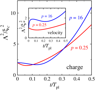
Figure 1: (Color online.) Inhomogeneity parameters of the charge density (main plot) and velocity (inset) pattern for two regimes of the Coulomb forces. The parameter $p\equiv\Omega_{\rm pl}\tau_{\rm eh}$ is shown near the plots. $p=16$ corresponds to the extremely weak damping, while for $p=0.25$ the damping is relatively strong. Here $T_{\rm pl}=0.9$ ps. The functions presented in the plots are universal in the sense they do not depend on the initial speed of the puddle $U_{0}$.

To trace the evolution in the inhomogeneity of the charge density and velocity patterns, we study $\xi_{c}$ and $\xi_{u}$, defined to be ratios of gross quantities:

$$\frac{1}{\xi_{c}^{2}(t)}{\int}N_{c}^{2}d^{2}r\equiv\int\left(\nabla N_{c}\right)^{2}d^{2}r,$$ (9)

$$\frac{1}{\xi_{u}^{2}(t)}\int\left(u_{x}-U\right)^{2}d^{2}r\equiv\int\left(\nabla u_{x}\right)^{2}d^{2}r,$$

that serve as characteristic lengths. Taking into account that the spatial inhomogeneity (internode distance) of the function $\psi_{n}(x)$ scales at large $n$ as $n^{-1/2}$, the number of harmonics forming the corresponding pattern scales as $\Lambda^{2}/\xi_{c}^{2}(t)$ or $\Lambda^{2}/\xi_{u}^{2}(t)$ if the distributions are strongly nonuniform. As one can see in Fig.1, both patterns, especially the density, become strongly inhomogeneous and the role and the number of the higher harmonics grows with time. Therefore, we expect that the spatial scales of the variations in the density and velocity will rapidly decrease. Eventually, a hydrodynamic description will fail, as stochastic behavior develops.chaos

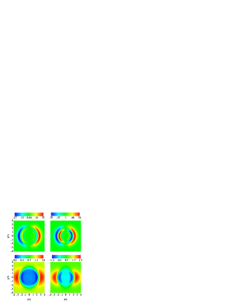
Figure 2: (Color online.) Patterns (in arbitrary, same for both columns, units) of charge density $N_{c}(x,y)$ (upper row) and velocity $u_{x}(x,y)$ (lower row) at $t=T_{\rm pl}/2$. Left column: $p=0.25$, right column: $p=16$. The density has $N_{c}(x,-y)=-N_{c}(x,y)$ symmetry. In the upper row, larger bow at $x>0$ corresponds to $N_{c}(x,y)>0$. The velocity satisfies the condition $u_{x}(-x,y)=u_{x}(x,y)$. For $u_{x}(x,y)$ maximum values are achieved at the wings $|x|/\Lambda$ close to 3, $y=0$. Minimum values are achieved at $|x|/\Lambda$ close to 1, $y=0$.

The underlying charge density is shown in the upper panel of Fig.2 where we plot the profiles $N_{c}(x,y,T_{\rm pl}/2)$. The lower panel shows the velocity $u_{x}(x,y,T_{\rm pl}/2)$. The profiles have a rather complex form, showing that the distributions of both quantities are strongly inhomogeneous.

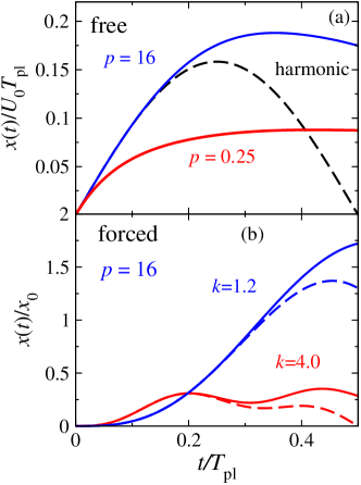
Figure 3: (Color online.) (a) Mean spot displacements for free spot propagation. Dashed line corresponds to the linear undamped oscillations. The displacement of the spot is on the order of $U_{0}T_{\rm pl}/4$, that is 20 nm for typical $U_{0}=100$ km/s and assumed here $T_{\rm pl}=0.9$ ps. (b) Mean spot displacements for the forced oscillations. Dashed lines correspond to the linear oscillator in Eq.(11). The frequency coefficients are $k=4$ (off-resonance) and $k=1.2$ (close to the resonance).

We calculate the mean spot displacement:

$$x(t)=\sum_{\overline{n}}\frac{N_{\overline{n}}^{e}}{N_{t}}\int x\Psi_{\overline{n}}\left(x,y\right)d^{2}r,$$ (10)

where $N_{t}=\pi N_{0}\Lambda^{2}$ is the total number of injected electrons. The displacement $x(t)$ has a complex time-dependence, after initially evolving simply as $U_{0}t$. Even at later times $x(t)$ is proportional to $U_{0}$ if all other parameters are kept the same. We show in Fig.3 the mean displacement $x(t)$ defined in Eq.(10) for two different cases presented in Fig.1: considerably ($p=0.25$) and very weakly ($p=16$) damped regimes. An astonishing result is the absence of the plasma oscillations even close to the clean limit with $p=16$. On the timescale of half of the expected oscillation period $T_{\rm pl}$, the spot becomes strongly inhomogeneous with harmonics up to $n_{1},n_{2}\leq 20$ contributing to the results. Therefore, no well-defined oscillations occur. In all cases considered, the maximum of $x(t)\sim U_{0}\min(T_{\rm pl},\tau_{\rm eh})$ is much less than $\Lambda$, and therefore the $\nabla{\mathbf{u}}$ and $\nabla{P}$-originated terms in the Euler equation can be neglected.

As another example of this unusual behavior, we present the results for the clean system ($p=16$) driven by an external field $\widetilde{E}(t)=E_{0}\sin(k\Omega_{\rm pl}t)$ for the same initial Gaussian density distribution as above, but with no current injection ($U_{0}=0$). Here the inhomogeneity develops more slowly than if current were injected, since $x(t)$ increases as $t^{3}$ rather than as $t$ at the initial stage of the process. Nonetheless, the $x(t)$ is considerably different from the expected for a linear oscillator:

$$x_{\rm lo}(t)=\frac{x_{0}}{1-k^{2}}\left(\sin k\Omega_{\rm pl}t-k\sin\Omega_{\rm pl}t\right),$$ (11)

with $x_{0}={eE_{0}}/m_{e}\Omega_{\rm pl}^{2}$, due to the fact that the excitation of the higher Hermite-Gaussian modes strongly influences the response to the external field, as shown in Fig. (3b). For a system driven close to resonance ($k=1.2$), the difference between the full and linear oscillator behavior is less than for $k=4$, since near resonance the uniform external force is more important than the interactions.

To conclude, the macroscopic dynamics of optically injected currents in clean semiconductor multiple quantum wells is strongly inhomogeneous and nonlinear, due to the nonuniform long-range Coulomb forces that develop. These forces arise following the initial breaking of the symmetry by the injected electron puddle velocity ${\bf U}_{0}$, which leads to a separation of electrons and holes that produces the nonuniform macroscopic Coulomb interaction. Due to the coupling of the Hermite-Gaussian modes through conservation of charge, the charge density becomes nonuniform on progressively smaller spatial scales. In contrast to what might be expected, it does not show well-defined plasma oscillations. The complex charge and current density patterns develop on a time scale on the order of a quarter of the plasma oscillation period characteristic of the given carrier density and puddle size. The length scales characterizing the spatial inhomogeneities in density and velocity decrease rapidly, and, in the terminology of Porkolab and Chang [Porkolab78, ], a turbulence regime will likely develop. These systems will provide a new laboratory example of plasmas with controlled non-linear behavior, and likely a transition to a stochastic regime.

Acknowledgement. This research was funded by the University of the Basque Country (grant GIU07/40), Natural Sciences and Engineering Research Council of Canada (NSERC) and the Ontario Centres of Excellence (OCE).

References

- (1) L. L. Bonilla and H. T. Grahn, Rep. Prog. Phys.68, 577 (2005)
- (2) K. Aoki, Nonlinear dynamics and chaos in semicondictors, Institute of Physics, Series in Condensed Matter Physics (2001); E. Scholl, Nonlinear Spatio-Temporal Dynamics and Chaos in Semiconductors, Cambridge Nonlinear Science Series, Cambridge University Press (2005).
- (3) C. Weber et al., Appl. Phys. Lett. 89, 091112 (2006)
- (4) N. Bushong et al., Phys. Rev. Lett. 99, 226802 (2007)
- (5) M. Porkolab and R. P. Chang, Rev. Mod. Phys. 50, 745 (1978)
- (6) R. C. Davidson et al., Rev. Mod. Phys. 63, 341 (1991)
- (7) T. Yamada et al., Nature Physics 4, 721 (2008)
- (8) H.M. van Driel and J.E. Sipe, In: K-T. Tsen, Editor, Ultrafast Phenomena in Semiconductors, Springer (2001) (Chapter 5).
- (9) R. Atanasov et al., Phys. Rev. Lett. 76, 1703 (1996), A. Hache et al., Phys. Rev. Lett. 78, 306 (1997), Ali Najmaie, R. D. Bhat, and J. E. Sipe, Phys. Rev. B 68, 165348 (2003)
- (10) H. T. Duc et al., Phys. Rev. B 74, 165328 (2006), H. T. Duc et al., Phys. Rev. Lett. 95, 086606 (2005)
- (11) Nonequlibrium Carrier Dynamics in Semiconductors (M. Saraniti and U. Ravaioli, Eds.), Spinger (2006)
- (12) R.M. Abrarov et al., Appl. Phys. Lett. 91, 232113 (2007).
- (13) H. Zhao et al., Phys. Rev. B 75, 075305 (2007), J.-Y. Bigot et al., Phys. Rev. Lett. 67, 636 (1991), W. A. Hügel et al., Phys. Status Solidi B 221, 473 (2000)
- (14) R.A. Hopfel et al., Phys. Rev. Lett. 56, 2736 (1986), R.A. Hopfel et al., Appl. Phys. Lett. 49, 573 (1986)
- (15) F. Steininger et al., Zeitschrift für Physik B 103, 45 (1997)
- (16) E.Ya. Sherman et al., Solid State Comm.139, 439 (2006)
- (17) T. Ando et al., Rev. Mod. Phys.54, 437 (1982)
- (18) The physical observables were calculated by summing the contributions of the states up to to avoid the influence of the upper states, which cannot be calculated reliably in the truncated basis.
- (19) H. Zhao et al., Journ. of Applied Physics, 103, 053510(2008)
- (20) L. D. Landau and E.M. Lifshitz Fluid Mechanics, Second Edition: Volume 6 (Course of Theoretical Physics).