Two-body problem in graphene

Abstract

We study the problem of two Dirac particles interacting through non-relativistic potentials and confined to a two-dimensional sheet, which is the relevant case for graphene layers. The two-body problem cannot be mapped into that of a single particle, due to the non-trivial coupling between the center-of-mass and the relative coordinates, even in the presence of central potentials. We focus on the case of zero total momentum, which is equivalent to that of a single particle in a Sutherland lattice. We show that zero-energy states induce striking new features such as discontinuities in the relative wave function, for particles interacting through a step potential, and a concentration of relative density near the classical turning point, if particles interact via a Coulomb potential. In the latter case we also find that the two-body system becomes unstable above a critical coupling. These phenomena may have bearing on the nature of strong coupling phases in graphene.

I Introduction

The problem of interactions in graphene layers was a subject of research even before its isolation and characterization in the laboratory Novoselov et al. (2004, 2005). It is peculiar due to its two-dimensional nature and to the honeycomb lattice structure into which ions are arranged. In the low-energy limit, the electronic properties are described by a Dirac-like equation for massless and chiral electrons Castro Neto et al. (2009). Undoped graphene has a vanishing density of states at the Fermi level and therefore a diverging screening length, so interactions are expected to yield a more singular behavior than in a conventional Fermi liquid picture, already well established in metals and electron gases Nozieres and Pines (1966); Giuliani and Vignale (2005). In fact, a weak-coupling scaling analysis was early performed González et al. (1994, 1999), shedding light on the role of electron-electron interactions mediated by the Coulomb potential: the resulting divergences in perturbation theory, once handled conveniently, turn out to have a small effect on the low energy properties of electrons, as they are marginally irrelevant in the renormalization group sense. However, that analysis does not exclude the possibility of phases with broken symmetry, where interactions play a major role, when the dimensionless coupling $g\equiv e^{2}/\epsilon\hbar v_{F}$ is of order unity or larger, $e$ being the electronic charge, $v_{F}$ the Fermi velocity, and $\epsilon$ the dielectric constant of the environment in which graphene is embedded Khveshchenko (2001); Gorbar et al. (2002); Khveshchenko and Leal (2004). This is expected to be the relevant case for graphene layers in vacuum, where $\epsilon=1$ and $g\simeq 2.16$. Along that direction, several works in the recent literature are pointing out the existence of exotic strong coupling phases in graphene layers, where pairing of electron and holes could give rise to an excitonic state, where a gap would be opened rendering the system insulating Khveshchenko (2001); Herbut et al. (2008); Drut and Lähde (2009a).

On the other hand, it is common wisdom in the field of strongly correlated systems, that the study of the interaction between two particles can provide important insights on the many-body physics. The relevance of this kind of studies in graphene has already been shown when addressing the Coulomb impurity problem Pereira et al. (2007); Shytov et al. (2007a, b); Novikov (2007). Here, a critical value of the coupling marks the breakdown of the Dirac vacuum, whose study requires consideration of the whole many-body problem. As pointed out recently Gamayun et al. (2009); Wang et al. (2009), there could be a relation between this instability and the formation of an excitonic condensate in the strongly-coupled many-body problem. Thus two-particle physics seems to underlie many features of the full many-body problem.

In this paper, we address the problem of two interacting Dirac electrons in two spatial dimensions, mediated by non-relativistic central potentials. This feature makes the problem different from the already well addressed fully relativistic problem. One of our goals is to shed light on the relation between the two-body problem and the many-body instabilities, so we pay special attention to the case of the bare Coulomb potential. However, the general problem happens to show peculiarities that make its separate study worthwhile. Importantly, the two-body problem cannot be mapped exactly into the one-body Coulomb impurity problem on the same lattice. In fact, we will show that the two-body problem presents remarkable differences, the most important being the singular role played by localized zero-energy states at those points where the kinetic energy vanishes. Interestingly, we find that, for zero center-of-mass momentum, the two-body problem in graphene is equivalent to that of a single particle in the lattice model proposed by Sutherland Sutherland (1986), where both lattices are considered in their continuum limit. The presence of zero-energy states can induce non-analyticities in the relative wave function, giving rise to partial localization phenomena for the Coulomb interacting case. In order to get a better understanding of the novel features, we address first the case of two particles interacting via a step potential.

The paper is organized as follows: Section II presents some general features of the two-body problem. Section III addresses the case of zero center-of-mass momentum, which is simpler to analyze and of potential relevance to many-body instabilities. Sections IV and V study the case of step and Coulomb potentials, respectively. Section VI discusses some aspects of the case of arbitrary center-of-mass momentum. Section VII is devoted to a discussion of the relation of the present work to many-body phenomena. Finally, section VIII summarizes the main conclusions. The paper includes three appendices where some technical issues have been collected.

II General features

As the main applications of this problem concern graphene sheets, we start with a formulation of the problem in terms of the continuum theory of graphene electron motion, which is known to be described by the Dirac equation. For a single particle, the wave function is a two-component spinor characterized by the quantum numbers of spin and valley, both with degeneracy two. For zero magnetic field and scalar translationally invariant interactions such as those which we will consider here, we can neglect the effect of those extra degrees of freedom and concentrate on the two-component spinor description. Later, we will discuss the effect of the spin. The single particle Dirac equation reads:

$$\left[\begin{array}[]{cc}v(r)&-i\partial_{x}-\partial_{y}\\ -i\partial_{x}+\partial_{y}&v(r)\end{array}\right]\left[\begin{array}[]{c}\Psi_{A}({\bf r})\\ \Psi_{B}({\bf r})\end{array}\right]=E\left[\begin{array}[]{c}\Psi_{A}({\bf r})\\ \Psi_{B}({\bf r})\end{array}\right]$$ (7)

where the pseudo-spin index $i=A,B$ refers to the two inequivalent sites within the unit cell of the honeycomb lattice.

Now let us consider the two particle problem. We construct two-particle wave functions from the tensor product of single-particle ones, $\Psi_{ij}({\bf r}_{1},{\bf r}_{2})\equiv\Psi_{i}({\bf r}_{1})\otimes\Psi_{j}({\bf r}_{2})$. This allows us to write the Schrödinger equation for the interacting problem, that in the language of four-component spinors reads:

$$\left[\begin{array}[]{cccc}v(r)&-i\partial_{x_{2}}-\partial_{y_{2}}&-i\partial_{x_{1}}-\partial_{y_{1}}&0\\ -i\partial_{x_{2}}+\partial_{y_{2}}&v(r)&0&-i\partial_{x_{1}}-\partial_{y_{1}}\\ -i\partial_{x_{1}}+\partial_{y_{1}}&0&v(r)&-i\partial_{x_{2}}-\partial_{y_{2}}\\ 0&-i\partial_{x_{1}}+\partial_{y_{1}}&-i\partial_{x_{2}}+\partial_{y_{2}}&v(r)\end{array}\right]\left[\begin{array}[]{c}\Psi_{AA}({\bf r}_{1},{\bf r}_{2})\\ \Psi_{AB}({\bf r}_{1},{\bf r}_{2})\\ \Psi_{BA}({\bf r}_{1},{\bf r}_{2})\\ \Psi_{BB}({\bf r}_{1},{\bf r}_{2})\end{array}\right]=E\left[\begin{array}[]{c}\Psi_{AA}({\bf r}_{1},{\bf r}_{2})\\ \Psi_{AB}({\bf r}_{1},{\bf r}_{2})\\ \Psi_{BA}({\bf r}_{1},{\bf r}_{2})\\ \Psi_{BB}({\bf r}_{1},{\bf r}_{2})\end{array}\right]$$ (8)

As we are dealing with translationally invariant potentials, we can switch to the center-of-mass frame, defining the new coordinates ${\bf R}=\frac{{\bf r}_{1}+{\bf r}_{2}}{2}$ and ${\bf r}={\bf r}_{1}-{\bf r}_{2}$. It is also convenient to apply the unitary transformation

$$\Psi_{1}=\Psi_{AA}$$

$$\Psi_{2}=\frac{1}{\sqrt{2}}(\Psi_{AB}+\Psi_{BA})$$

$$\Psi_{3}=\frac{1}{\sqrt{2}}(\Psi_{AB}-\Psi_{BA})$$

$$\Psi_{4}=\Psi_{BB}$$ (9)

and use a plane wave ansatz for the center-of-mass part of the wave function, $\Psi_{i}({\bf R},{\bf r})=e^{i{\bf K}\cdot{\bf R}}\psi_{i}({\bf r})$. We arrive at the following eigenvalue problem:

$$\left[\begin{array}[]{cccc}v(r)&\frac{1}{\sqrt{2}}Ke^{-i\theta_{K}}&\sqrt{2}e^{-i\phi}(i\partial_{r}+\frac{1}{r}\partial_{\phi})&0\\ \frac{1}{\sqrt{2}}Ke^{i\theta_{K}}&v(r)&0&\frac{1}{\sqrt{2}}Ke^{-i\theta_{K}}\\ \sqrt{2}e^{i\phi}(i\partial_{r}-\frac{1}{r}\partial_{\phi})&0&v(r)&-\sqrt{2}e^{-i\phi}(i\partial_{r}+\frac{1}{r}\partial_{\phi})\\ 0&\frac{1}{\sqrt{2}}Ke^{i\theta_{K}}&-\sqrt{2}e^{i\phi}(i\partial_{r}-\frac{1}{r}\partial_{\phi})&v(r)\end{array}\right]\left[\begin{array}[]{c}\psi_{1}\\ \psi_{2}\\ \psi_{3}\\ \psi_{4}\end{array}\right]=E\left[\begin{array}[]{c}\psi_{1}\\ \psi_{2}\\ \psi_{3}\\ \psi_{4}\end{array}\right]\,,$$ (10)

where $\theta_{K}\equiv\arctan(K_{y}/K_{x})$ and polar coordinates are used for the relative coordinate. As a first remark on this equation, we notice that the center-of-mass coordinate does not decouple from the relative one, even though the potential only depends on the latter. This is a consequence of the chiral nature of the electron carriers, where pseudo-spin and momentum are coupled. This kind of coupling also prevents the Hamiltonian from commuting with the relative angular momentum, thus frustrating a possible decomposition of the problem in terms of partial waves.

III The case $K=0$

In order to gain insight into the many-body problem, the most interesting case is that of zero total center-of-mass momentum. Then the two particles have opposite momenta, like in the Cooper channel in metals. Any pairing effect should be particularly important in this energetically most favorable case. It is also the simplest one, because it decouples the second component $\psi_{2}(r)$ from the rest. In effect, the equation for this component reads

$$[v(r)-E]\psi_{2}(r)=0$$ (11)

whose solution is $\psi_{2}(r)=0$ except at the particular point $v(r)=E$, if it exists. That point having measure zero, we will ignore the $\psi_{2}$ component as physically irrelevant. However, we will see later that, at the point where $v(r)=E$ is satisfied, zero-energy states are responsible for important non-analyticities in the other components.

We are thus left with an effective three-component problem. Remarkably, the $K=0$ Hamiltonian commutes with the relative angular momentum, so we can use the following ansatz for the wave function:

$$\left[\begin{array}[]{c}\psi_{1}(r)\\ \psi_{3}(r)\\ \psi_{4}(r)\end{array}\right]\equiv\left[\begin{array}[]{c}e^{i(l-1)\phi}\phi_{1}(r)\\ -\frac{i}{\sqrt{2}}e^{il\phi}\phi_{2}(r)\\ e^{i(l+1)\phi}\phi_{3}(r)\end{array}\right]$$ (12)

where the prefactors have been chosen for convenience. The labeling of the components in Eq. (12) has been changed in order to accommodate it to the three-component case. After using this ansatz, the system of equations reads:

$$\left[\begin{array}[]{ccc}v(r)-E&\partial_{r}+\frac{l}{r}&0\\ -2(\partial_{r}-\frac{l-1}{r})&v(r)-E&2(\partial_{r}+\frac{l+1}{r})\\ 0&-\partial_{r}+\frac{l}{r}&v(r)-E\end{array}\right]\left[\begin{array}[]{c}\phi_{1}(r)\\ \phi_{2}(r)\\ \phi_{3}(r)\end{array}\right]=0$$ (13)

It is interesting to note that these equations, as well as those directly derived from the full Hamiltonian for $K=0$, Eq. (10), can also be obtained as the continuum limit of a one-particle lattice Hamiltonian, defined in a triangular lattice with three sites in the unit cell, as initially considered by SutherlandSutherland (1986). A scheme of this lattice is shown in Fig. 1.

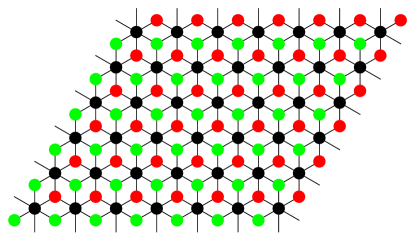
Figure 1: Scheme of the lattice proposed by Sutherland in Ref. Sutherland, 1986. The two-body problem in the low-energy sector of the honeycomb lattice, for $K=0$, is mathematically equivalent to a single-particle problem in this lattice. Zero-energy states in the Sutherland lattice appear due to the existence of a flat band.

Within this formulation, the case $l=0$ is the most symmetric one:

$$\psi(r)=\left[\begin{array}[]{c}e^{-i\phi}\phi_{1}(r)\\ -\frac{i}{\sqrt{2}}\phi_{2}(r)\\ e^{i\phi}\phi_{3}(r)\end{array}\right]\,.$$ (14)

Henceforth, we will refer to it as the $s$-wave, and as we will see, simple solutions can be obtained for this case taking advantage of its symmetry.

III.1 Symmetry properties

Let us now analyze the symmetry properties of the $K=0$ solutions. In the original basis, the two-body wave functions read:

$$\left[\begin{array}[]{c}\Psi_{AA}({\bf r}_{1},{\bf r}_{2})\\ \Psi_{AB}({\bf r}_{1},{\bf r}_{2})\\ \Psi_{BA}({\bf r}_{1},{\bf r}_{2})\\ \Psi_{BB}({\bf r}_{1},{\bf r}_{2})\end{array}\right]_{K=0}=\left[\begin{array}[]{c}e^{i(l-1)\phi}\phi_{1}(r)\\ -\frac{i}{2}e^{il\phi}\phi_{2}(r)\\ \frac{i}{2}e^{il\phi}\phi_{2}(r)\\ e^{i(l+1)\phi}\phi_{3}(r)\end{array}\right]\,,$$ (23)

where the symmetric combination has been taken $\psi_{2}=0$, as argued above. This wave function has a spinorial structure, due to the pseudo-spin of the particles, and a spatial structure coupled to the former. The symmetry properties under exchange of particles are studied by doing the transformation:

$${\bf r}_{1}\rightleftharpoons{\bf r}_{2}$$

$$\Psi_{AB}\rightarrow\Psi_{BA}\,.$$ (24)

The first transformation, for $K=0$, translates into $\phi\rightarrow\phi+\pi$. It follows inmediatly that wave functions with $l$ even are antisymmetric under particle exchange, while those with $l$ odd are symmetric. Hence, the $s$-wave is, interestingly, antisymmetric. This somewhat counterintuitive result reflects the role of the sublattice pseudo-spin in the orbital wave function.

This has consequences on the total wave functions, once both spin and valley degrees of freedom are also considered. Everywhere in this article we assume that the two particles belong to the same valley. Since their total wave function must be antisymmetric, the following two families of solutions appear:

$$\begin{array}[]{cc}\rm{(i)}&\Psi_{K=0,l=\rm{odd}}({\bf r}_{1},{\bf r}_{2})\otimes\frac{1}{\sqrt{2}}\left(|\uparrow\downarrow\rangle-|\downarrow\uparrow\rangle\right)\\ \rm{(ii)}&\Psi_{K=0,l=\rm{even}}({\bf r}_{1},{\bf r}_{2})\otimes|\uparrow\uparrow\rangle\\ &\Psi_{K=0,l=\rm{even}}({\bf r}_{1},{\bf r}_{2})\otimes|\downarrow\downarrow\rangle\\ &\Psi_{K=0,l=\rm{even}}({\bf r}_{1},{\bf r}_{2})\otimes\frac{1}{\sqrt{2}}\left(|\uparrow\downarrow\rangle+|\downarrow\uparrow\rangle\right)\end{array}$$ (29)

Therefore, the lowest angular-momentum channel ($l=0$) corresponds to a triplet spin-state, as opposed to what happens with ordinary Schrödinger electrons.

III.2 Other mathematical properties

Equation (13) comprises three coupled differential equations. Adding the first and the third equations we may solve for $\phi_{2}$ in terms of $\phi_{1}$ and $\phi_{3}$:

$$\phi_{2}=\frac{r}{2l}\varepsilon(r)(\phi_{1}+\phi_{3})~{},$$ (30)

where $\varepsilon(r)\equiv E-v(r)$. Substracting the same two equations, we obtain

$$\partial_{r}\phi_{2}=\varepsilon(r)(\phi_{3}-\phi_{1})~{}.$$ (31)

Differentiating Eq. (30) and relating the result to Eq. (31), we obtain

$$\partial_{r}[\varepsilon(\phi_{1}+\phi_{3})]=\frac{\varepsilon}{r}\left[(2l-1)\phi_{3}-(2l+1)\phi_{1}\right]~{}.$$ (32)

On the other hand, the second equation of system (13) can be rewritten as:

$$\partial_{r}(\phi_{1}-\phi_{3})=\left(\frac{l-1}{r}-\frac{\varepsilon^{2}r}{4l}\right)\phi_{1}+\left(\frac{l+1}{r}-\frac{\varepsilon^{2}r}{4l}\right)\phi_{3}~{}.$$ (33)

Thus, system (13) can be solved in principle by first solving for $\phi_{1}$ and $\phi_{3}$ from (32) and (33) and then obtaining $\phi_{2}$ from (30). The absolute values of $\phi_{1}$ and $\phi_{2}$ should remain bounded as long as $\varepsilon(r)$ is bounded. A problem may appear for $r\rightarrow 0$ in the case of the Coulomb potential ($v(r)\sim r^{-1}$). In such a case, we will see that regular solutions can be obtained analytically for $r\rightarrow 0$, yielding in fact a useful starting point to initiate the numerical integration.

Another important issue arises when $\varepsilon\rightarrow 0$, i.e., at those points where the kinetic energy vanishes, whenever $l>0$. For a smooth potential, a linear approximation of $\varepsilon(r)$ around the vanishing point $r_{0}$ holds, $\varepsilon(r)=\lambda x+{\mathcal{O}}(x^{2})$, where $x\equiv r-r_{0}$. The differential equations (32) and (33) can be approximated around this point, yielding:

$$\frac{d}{dx}\left[x(\phi_{1}+\phi_{3})\right]\simeq 0$$ (34)

$$\frac{d}{dx}(\phi_{1}-\phi_{3})\simeq-\frac{1}{r_{0}}(\phi_{1}+\phi_{3})$$ (35)

The solution for these equations reads $\phi_{1}+\phi_{3}\simeq-2C_{2}/x$ and $\phi_{1}-\phi_{3}\simeq 2C_{1}+(2C_{2}/r_{0})\log(x)$. We see that, for $l>0$, a smooth potential will show non-analyticities close to $r_{0}$ in $\phi_{1}$ and $\phi_{3}$, while $\phi_{2}$ will remain continuous:

$$\phi_{1} \simeq C_{1}+\frac{C_{2}}{r_{0}}\log(x)-\frac{C_{2}}{x}$$

$$\phi_{2} \simeq \frac{\lambda r_{0}}{2l}C_{2}$$

$$\phi_{3} \simeq -C_{1}-\frac{C_{2}}{r_{0}}\log(x)-\frac{C_{2}}{x}$$ (36)

Notice, however, that these non-analyticites give a finite contribution to the probability $\int dr\,r\,|\phi|^{2}$. Therefore they are physical solutions of the Dirac equation.

We end by noting that this singular behavior remains unaltered even in the pres- ence of a small mass in the two-electron Dirac equation. Mathematically, this happens because the mass terms in the equations are subleading in the short-distance expansion around the point $r_{0}$.

IV Step potential

Some physical insight into the subtle properties of the interacting two-particle problem can be obtained by considering the simpler case of a step potential, which is typically considered a good effective description of the more general class of short-range potentials:

$$v(r)=\left\{\begin{array}[]{lr}v_{0}&r<r_{0}\\ 0&r>r_{0}\end{array}\right.$$ (37)

As usual, the procedure is to construct the solutions for each region and eventually match them, as shown schematically in Fig. 2.

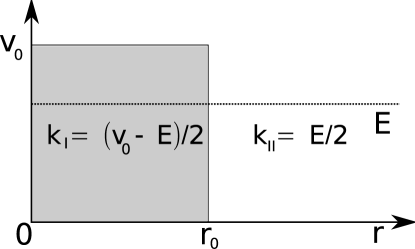
Figure 2: Scattering of two particles interacting through a short range potential.

For arbitrary energy $E$, the solutions are given by Bessel functions of the form:

$$\chi_{1}=\left[\begin{array}[]{c}aJ_{l-1}(kr)\\ bJ_{l}(kr)\\ cJ_{l+1}(kr)\end{array}\right],\,\chi_{2}=\left[\begin{array}[]{c}aY_{l-1}(kr)\\ bY_{l}(kr)\\ cY_{l+1}(kr)\end{array}\right]$$ (38)

where the coefficients and the eigenvalues are determined from the diagonalization of Eq. (13), the result being

$$E = v_{0}+2k,\,\,\,\,\left(\begin{array}[]{ccc}\frac{1}{2},&1,&\frac{1}{2}\end{array}\right)$$ (40)

$$E = v_{0}-2k,\,\,\,\,\left(\begin{array}[]{ccc}\frac{1}{2},&-1,&\frac{1}{2}\end{array}\right)$$ (42)

$$E = v_{0},\,\,\,\,\frac{1}{\sqrt{2}}\left(\begin{array}[]{ccc}1,&0,&-1\end{array}\right)$$ (44)

the normalization being chosen to simplify the global wave function, Eq. (12). The first solution corresponds to two electrons located in the upper Dirac cone, while in the second solution the two electrons are in the lower cone. The third solution describes the case where one particle is in the upper cone and the other one in the lower cone. Due to the zero total center-of-mass momentum, this solution has zero total energy. Notice that, for fixed $E$, the relation of $k$ with the energy depends on the solution chosen. The third one is valid for arbitrary $k$. Importantly, when $E=v_{0}$ there are other zero-energy states that are also solutions of the two-particle Dirac equation. They have the form

$$\chi_{3}=\frac{r^{\alpha}}{[1+(\frac{\alpha-l+1}{\alpha+l+1})^{2}]^{1/2}}\left(\begin{array}[]{ccc}1,&0,&\frac{\alpha-l+1}{\alpha+l+1}\end{array}\right)\,,$$ (46)

where $\alpha$ is a continuous parameter that can take any real value. These polynomial solutions are in general non-physical, as they cannot be properly normalized. However, they can be considered responsible for the non-analyticities shown to exist at those points where the kinetic energy vanishes (see section III.B). For the step potential, which is non-analytic itself, the existence of zero-energy states induces discontinuities in the radial wave function, thus changing the usual matching conditions. How such an anomalous behavior arises is explained in detail in Appendix A. Notice that in the presence of a mass this kind of solutions still exist, since they involve large derivatives within a narrow distance range.

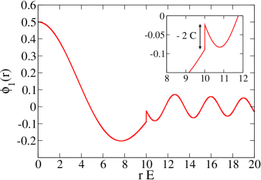
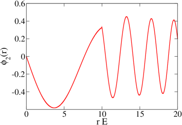
Figure 3: Numerical solution of the step-potential for $K=0$ and $l=1$ ($r_{0}E=10$, $E=v_{0}/2$). Top: first component of the radial wave function. The discontinuity induced by the zero energy states arises naturally in the numerical solution. Bottom: second component of the radial wave function. As also predicted by the new matching conditions, the second component does not have a d iscontinuity

We note that the traditional criterion of imposing continuity of the wave functions does not work here due to the insufficient number of matching parameters. To exemplify this issue, let us consider the situation shown in Fig. 2, where $k_{I}=(v_{0}-E)/2>0$ and $k_{II}=E/2>0$. The solution for region I only includes Bessel functions of the first kind, $J_{l}(k_{I}r)$, as those of the second kind ones are singular at the origin. Hence $\phi_{i}^{I}\sim A_{1}J_{l_{i}}(k_{I}r)$. For region II both solutions must be considered, $\phi_{i}^{II}\sim B_{1}J_{l_{i}}(k_{I}r)+B_{2}Y_{l_{i}}(k_{II}(r)$. Due to the freedom for global normalization, only two relative values of the three constants are relevant. Thus only two parameters remain to satisfy the continuity of three equations, one for every component of the wave function, leaving the problem overdetermined.

In Appendix A it is shown that, when zero-energy states at the matching point are taken into account, a third matching parameter arises naturally which permits a discontinuity in the radial wave function. Namely, we obtain

$$\Delta\phi_{1}(r_{0})\equiv\phi_{1}^{II}(r_{0})-\phi_{1}^{I}(r_{0}) = -2C$$

$$\Delta\phi_{2}(r_{0}) = 0$$

$$\Delta\phi_{3}(r_{0}) = -2C\,,$$ (47)

where $C$ is the extra parameter to determine. With the new matching conditions, an exact solution of the $K=0$ case becomes possible, as detailed in Appendix B. It is also interesting to compute the solution of the differential equations numerically, as shown in Fig. 3. Here, the first two components of the radial wave function are plotted. As predicted in equation (47), the first component shows a discontinuity induced by zero-energy states at the point $r=r_{0}$. The same consideration applies to the third component (not shown) but not for the second one.

It is also worth noting that, as expected, the $s$-wave shows a simpler behavior by virtue of its symmetric form. In this case, inspection of Eq. (13) shows $\phi_{1}(r)=-\phi_{3}(r)$ and the problem reduces to a two-component one. The matching conditions reduce then to continuity and the $s$-wave problem essentially behaves as that of the single particle. As a corollary, Eq. (47) leads to $C=0$ in this case. Thus we may state that the $l=0$ case has a structure similar to that of the impurity one-body problem in graphene.

V Coulomb potential

We now turn to the more relevant case of a long-range Coulomb potential, $v(r)=g/r$, where $g=e^{2}/\epsilon\hbar v_{F}$ for low-energy graphene electrons. It is convenient to find a more suitable form of Eq. (13) in order to obtain analytical solutions when possible. This is done by the usual procedure of analyzing the short and long distance limits. At short distances the wave function components have the form $\phi_{i}(r\rightarrow 0)\sim r^{\gamma-1/2}$, with $\gamma^{2}=\frac{1}{4}(1+4l^{2}-g^{2})$. On the other hand, the long-distance wave function behaves like a plane wave of the form $\phi_{i}(r\rightarrow\infty)\sim e^{\pm iEr/2}$. Hence, we can make the following ansatz for the radial wave function:

$$\phi_{i}(\rho)=\rho^{\gamma-1/2}e^{-\rho/2}\hat{\phi_{i}}(\rho)$$ (48)

where we have introduced the dimensionless radial complex coordinate $\rho=iEr$. By applying this transformation, Eq. (13) becomes

$$\left[\begin{array}[]{ccc}i\rho+g&\rho\partial_{\rho}-\frac{\rho}{2}+\gamma+l-\frac{1}{2}&0\\ -2(\rho\partial_{\rho}-\frac{\rho}{2}+\gamma-l+\frac{1}{2})&i\rho+g&2(\rho\partial_{\rho}-\frac{\rho}{2}+\gamma+l+\frac{1}{2})\\ 0&-\rho\partial_{\rho}+\frac{\rho}{2}-\gamma+l+\frac{1}{2}&i\rho+g\end{array}\right]\left[\begin{array}[]{c}\hat{\phi}_{1}(\rho)\\ \hat{\phi}_{2}(\rho)\\ \hat{\phi}_{3}(\rho)\end{array}\right]=0\,.$$ (49)

The general case is difficult to handle and only the $s$-wave channel admits an analytical solution, since it reduces to an effective single particle problem. The details of this solution are summarized in Appendix C. For general angular momentum $l$, Eq. (49) must be solved numerically.

Before addressing the full solution, let us point out the remarkable behavior of the wave functions at short distances. As we have seen, it goes like a power law $r^{\gamma-1/2}$, where $\gamma=\frac{1}{2}\sqrt{1+4l^{2}-g^{2}}$. For $|g|<g_{c}\equiv\sqrt{1+4l^{2}}$ only $\gamma>0$ is acceptable. By contrast, for $|g|>g_{c}$, the $\gamma$ parameter becomes imaginary and the wave function shows a pathological short-distance behavior, going like $r^{-1/2}[\cos(|\gamma|\log r)\pm i\sin(|\gamma|\log r)]$. Thus the wave function oscillates dramatically towards the center. This kind of behavior was already found in the Coulomb impurity problem, where it was related to an instability of the wave function that could signal the breakdown of the Dirac vacuum. For strong enough couplings, the two-particle interaction would produce electron-hole pairs from the vacuum, and a full quantum field-theoretical treatment of the problem could be necessary. The consequences for the two-body problem of this effect have not been addressed in this paper, although from the study of the Coulomb impurity problem, we may expect a non-linear screening as a result of the reorganization of the many-body vacuum. Shytov et al. (2007b)

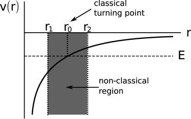
Figure 4: Sketch of the Coulomb potential (attractive, in this case), including all the relevant lenght scales discussed in the text. $E$ is the total energy of the particle, $r_{0}$ is the classical turning point, and the region between $r_{1}$ and $r_{2}$ is the classically forbidden region.

In order to gain further insight into the instability, a semiclassical analysis like that performed in Ref. Shytov et al., 2007a can be applied. Our starting point is Eq. (13) for the Coulomb potential with the ansatz $\phi_{i}(r)=\bar{\phi}_{i}\frac{e^{i2p_{r}r}}{\sqrt{r}}$, where $p_{r}$ is a slowly varying function of $r$. This justifies the assumption $\partial_{r}p_{r}\simeq 0$. Equation (13) then reads

$$\left[\begin{array}[]{ccc}\frac{g}{r}-E&i2p_{r}+\frac{l-1/2}{r}&0\\ -i4p_{r}+\frac{2l-1}{r}&\frac{g}{r}-E&i4p_{r}+\frac{2l+1}{r}\\ 0&-i2p_{r}+\frac{l+1/2}{r}&\frac{g}{r}-E\end{array}\right]\left[\begin{array}[]{c}\bar{\phi_{1}}\\ \bar{\phi_{2}}\\ \bar{\phi_{3}}\end{array}\right]=0\,.$$ (50)

The determinant vanishes if one of the following relations is satisfied:

$$\frac{g}{r}=E\,,$$ (51)

$$p_{r}^{2}=(\frac{g}{r}-E)^{2}-\frac{1}{r^{2}}(4l^{2}+1)\,.$$ (52)

The first equation defines a point, $r_{0}\equiv g/E$, where any function $p_{r}$ gives a solution thanks to the existence of zero-energy states, as discussed in the previous section for the step potential. Notice that this condition only is fulfilled for repulsive electrons with positive energy or attractive electrons with negative energy, two cases which are related through a symmetry transformation. The second equation, on the other hand, defines a non-classical region where $p_{r}^{2}<0$. The region is $r_{1}<r<r_{2}$, where $r_{1,2}=\frac{g}{E}\mp\frac{1}{E}\sqrt{4l^{2}+1}$. Remarkably, we see that $r_{1}<r_{0}<r_{2}$, i.e. the point where zero-energy states nucleate belongs to this classically forbidden region, as sketched in Fig. 4.

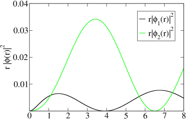
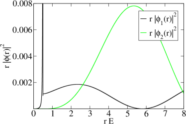
Figure 5: Numerical solution of the radial wave function for the case of Coulomb interaction and zero center-of-mass momentum. The chosen angular momentum is $l=1$. Top: wave functions for $g=-0.5$ and $E>0$. Bottom: wave functions for $g=0.5$ and $E>0$. Notice that, where the condition $g/r_{0}=E$ is satisfied, a singularity is induced by the localized zero-energy states.

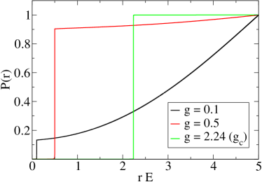
Figure 6: Probability of finding one electron within a distance $r$ from the other electron, $P(r)=\sum_{i}\int_{0}^{r}d^{2}r|\phi_{i}({\bf r})|^{2}$, for $K=0$, $l=1$, and various values of the dimensionless Coulomb coupling constant $g$, in the important case where a classical turning point exists ($rE=g$). Here, the influence of zero-energy states translates into (i) a suppression of the electron density for $r<r_{0}$, and (ii) a tendency to concentrate the probability near $r=r_{0}$ as the critical coupling $g_{c}$ is approached. The results are normalized to their value at $rE=5$.

The Coulomb problem still presents other peculiarities. In Fig. 5, a numerical estimate of the radial wave functions is shown for $l=1$ and two different signs of the interaction below the critical value. The main feature in this solution concerns again zero-energy states: when the condition $g/r_{0}=E$ is fulfilled, zero-energy states must be taken into account and become responsible for singularities in the first and third components of the wave function when $l\neq 0$, as shown above on general grounds. In the Coulomb case, this effect has remarkable consequences, such as a drastic suppression of the probability of finding the particle in $r<r_{0}$, and a tendency to increasingly localize the radial wave function near $r=r_{0}$ when the critical point $g_{c}$ is approached from below (see Fig. 6). We find numerically that for $g=g_{c}$ the relative wave function becomes effectively localized near $r=r_{0}$.

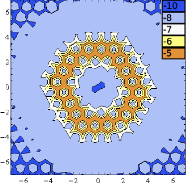
Figure 7: Logarithmic density distribution of the two-particle wave function interacting with a Coulomb potential (see text for details), for $K=0$. One of the particles is assumed to be placed at the center of the square. The equations are discretized using the Sutherland lattice, and the energy range of the integrated states is chosen such that they cover the region where the condition $g=r_{0}E$ is fulfilled. As expected, the results show a clear concentration of the density at this point $r_{0}$. The short-length features of the density plot reflect the underlying lattice structure.

These results are similar to those obtained for a single particle in the Sutherland lattice Sutherland (1986) with a Coulomb potential. As shown in Fig. 7, we use a $30\times 30$ lattice with the structure of Ref. Sutherland, 1986 (see Fig. 1) and periodic boundary conditions. The potential is $v(r)=v_{0}e^{-r/r_{d}}/\sqrt{r^{2}+r_{1}^{2}}$, with $v_{0}=t>0,r_{d}=20a$ and $r_{1}=0.5a$, where $t$ is the hopping, and $a$ is the distance between nearest neighbor equivalent atoms. The states considered to construct the density plots are in the range of energies $0.25t\leq E\leq 0.35t$. Since they are not eigenstates of the Hamiltonian, they are expected to contain several angular channels. However, as shown in Fig. 7, this energy spread is sufficient to find an enhancement of the density in the region near $E=v(r)$. When states in the range $E<0$ are considered, the density shows a delocalized distribution. In the plots, notice that there are details coming from the underlying lattice structure that are not relevant for our discussion, since we focus on the continuum limit.

In case of considering a small mass in the prob- lem, the two most prominent features of the Coulomb two-body problem, i.e., the instability above a critical coupling and the influence of zero-energy states, are not essentially altered. The Coulomb instability has its origin in the short-distances behaviour of the wave function, where mass terms are subleading. These terms are also subleading in the expasion around the classical turning point r0, thus not helping to prevent the appearance of non-analyticities caused by zero-energy states which also exist for nonzero mass.

VI Extension to finite $K$

The most salient features we have found in the problem of two interacting particles are, so far, the influence of zero-energy states and the appearance of instabilities for the Coulomb potential. Next we ponder to what extent those results still apply for the general case of nonzero center-of-mass momentum.

Zero-energy states are investigated by taking $v(r)=E$ in the eigenvalue problem (10). Inspection of the resulting Hamiltonian reveals that it separates into two independent sectors. Hence, the Hilbert space of solutions is two-dimensional, with the general solution for the zero-energy states reading now

$$\psi(r,\phi)=A_{1}\left[\begin{array}[]{c}r^{\alpha}\sin^{\alpha}(\theta_{K}-\phi)\\ 0\\ 0\\ -r^{\alpha}\sin^{\alpha}(\theta_{K}-\phi)\end{array}\right]$$ (57)

$$+A_{2}\left[\begin{array}[]{c}0\\ \frac{K}{2}r^{\beta}\sin^{\beta}(\theta_{K}-\phi)\\ r^{\beta-1}\sin^{\beta-1}(\theta_{K}-\phi)\\ 0\end{array}\right]\,,$$ (62)

where $A_{1}$ and $A_{2}$, as well as $\alpha$ and $\beta$, can take arbitrary values. A similar analysis to that of $K=0$ can be performed here. For the case of a step potential, they translate into a change in the matching conditions, since the introduction of two new parameters ($B_{1}$ and $B_{2}$) changes the continuity of the wave function:

$$\Delta\psi_{1}(r_{0},\phi) = B_{1}(\phi,K,\theta_{K})$$

$$\Delta\psi_{2}(r_{0},\phi) = B_{2}(\phi,K,\theta_{K})$$

$$\Delta\psi_{3}(r_{0},\phi) = 0$$

$$\Delta\psi_{4}(r_{0},\phi) = -e^{2i\theta_{K}}B_{1}(\phi,K,\theta_{K})$$ (63)

Linearization of the equations close to the point where $\varepsilon(r)=0$ (the classical turning point) shows that, even for smooth potentials, singularities in the relative wave functions arise. Still, they are square integrable and give a finite contribution to the probability.

As for the Coulomb instability, its existence can be probed by checking the short-distance limit of the full Hamiltonian given in (10), for the case $v(r)=g/r$. It is not difficult to see that the small $r$ limit is controlled by $K$-independent terms. Thus, for $r\rightarrow 0$ we recover the $K=0$ limit, where an instability has already been identified. Hence, we expect this instability to be a general feature of the Coulomb problem.

VII Relevance to many-body phenomena

As mentioned in the Introduction, it can be expected on general grounds that the two-body problem with Coulomb interactions provides information on the more complicated many-body problem in graphene. This is especially relevant in the strong-coupling regime, as several works in the literature suggest the possibility of a new insulating phase above a certain critical coupling, where electron and holes would bind forming excitons and opening up a gap.

It has been pointed out in the literature Gamayun et al. (2009); Wang et al. (2009), that the breakdown of the Dirac vacuum in the attractive Coulomb impurity problem could be related to such a formation of excitons in graphene for strong enough coupling. We have seen in this article that this behavior is also present in the two-body problem, which should be even more relevant to the many-body physics

In order to understand the connection, we must notice that in principle the problem of an interacting electron and hole can be mapped into that of two attractive electrons, with similar symmetry properties. However, like for the Coulomb impurity problem, a more rigorous mapping would be performed by considering the existence of the Dirac sea, which constraints, by Pauli’s principle, the states accessible to the electron-hole pair, in analogy to the Cooper problem Schrieffer (1999). Such a treatment, however, would require to work in a different basis for which the analytical results obtained in this paper do not hold , and is thus beyond the scope of this paper.

We note in this regard that the breakdown of the Dirac vacuum in the two-body problem could be a signature of the excitonic instability in the many-body system. As we have already shown, the critical value for which the breakdown occurs depends on the scattering channel. For the most symmetric one, the $s$-wave, we find $g_{c}=1$, which should be compared to the critical values obtained for the Coulomb impurity problem, $g_{c}^{{\rm CI}}=0.5$. Pereira et al. (2007); Shytov et al. (2007a, b); Novikov (2007) For higher angular-momentum channels the critical couplings increase. As an example, $g_{c}=2.24$ for $l=1$. However, at low energies those higher angular momenta are usually less important. Hence, the $s$-wave critical coupling should provide an educated guess of the corresponding value for the expected many-body instability. Remarkably, the critical values obtained so far in the theoretical literature are close to the value predicted here for the two-body problem. Monte Carlo calculations in the lattice give a critical coupling $g_{c}^{{\rm MC1}}\simeq 1.11$ Drut and Lähde (2009a, b) and $g_{c}^{{\rm MC2}}\simeq 1.66$, Armour et al. (2009) depending on the model used to simulate graphene electrons. Renormalization Group calculations yield $g_{c}^{{\rm RG}}\simeq 0.833$. Vafek and Case (2008) Finally, a variational approach to the excitonic condensate has been recently reported to show a transition above the critical coupling $g_{c}^{{\rm var}}\simeq 1.13$. Khveshchenko (2009) The two-body problem with Coulomb interactions of strength above the critical coupling has not been addressed in this paper. As mentioned above, from the study of the Coulomb impurity problem it can be expected that the instability, which produces a reorganization of the Dirac vacuum, leads to a non-linear screening of the interactions. Shytov et al. (2007b) This effect should be analyzed carefully in order to establish its connection with a possible formation of excitons, where it could happen that still the presence of the Dirac sea as a constraint is necessary in order to produce a bound state. After all, the results presented in this paper do not shed sufficient light on the consequences of the actual many-body instability.

Regarding the spin degree-of-freedom, as discussed in section II, if both electrons belong to the same valley the $s$-wave channel would correspond to a triplet state in the spin sector. This fact may be highly relevant for the study of the excitonic instability in the presence of an external magnetic field.

There is a second aspect of the two-body problem in graphene that could have consequences on the more complicated many-body problem: the influence of zero-energy states for $l\neq 0$ angular momentum channels. As we have seen, in those cases where the kinetic energy vanishes at some point (positive total energy and repulsive potential, or negative total energy and atractive potential), zero-energy states induce singularities in the wave function which translate into an increasing probability of finding the particle at the classical turning point $r_{0}$, when the critical coupling $g_{c}$ is approached.

Let us discuss the role of the carrier density in this scenario. We only consider couplings below the critical one in case of Coulomb interactions, since we expect a description in terms of linear screening to be applicable. In doped graphene, electrons at the Fermi surface have an energy $E_{F}=v_{F}k_{F}=v_{F}(4\pi n/N_{s})^{1/2}$, where $n$ is the electron density in the upper cone and $N_{s}=4$ the valley and spin degeneracy. This defines a classical return distance $r_{0}\equiv g/E_{F}\propto n^{-1/2}$ for the Fermi surface electrons at which density correlation should peak. On the other hand, the static screening of the Coulomb interaction in doped graphene is characterized by the Thomas-Fermi (TF) screening length $\lambda_{\mathrm{TF}}=g^{-2}(4\pi nN_{s})^{-1/2}$,Ando (2006); Wunsch et al. (2006); Hwang and DasSarma (2007) which shows a similar density dependence, namely, $\lambda_{\mathrm{TF}}\propto n^{-1/2}$. Thus the ratio between the classical return and screening distances is independent of the density: $r_{0}/\lambda_{\mathrm{TF}}=N_{s}g^{2}$. For many cases we expect $r_{0}/\lambda_{\mathrm{TF}}>1$, which places $r_{0}$ beyond the screening length, i.e. where the bare Coulomb interaction, for which $r_{0}$ has been calculated, does not hold. Naively this might invalidate the physics associated to zero-energy states, which is expected to occur at $r=r_{0}$. However, it is easy to note that the density correlation peaks have to be a robust feature of the many-body problem.

We have seen that zero-energy states intervene at the point where $v(r)=E$. It is quite reasonable to assume that, in a many-body context, that condition must be replaced by $v_{\mathrm{scr}}(r_{0})=E_{F}$, which defines the classical return distance $r_{0}$ for the electron gas if $v_{\mathrm{scr}}(r)$ is the screened Coulomb interaction potential. Within the TF approximation, the screened potential has the form Ando et al. (1982); Giuliani and Vignale (2005) $v_{\mathrm{scr}}(r_{0})=(e^{2}/r)F(r/\lambda_{\mathrm{TF}}),$ where $F(x)$ is a monotonically decreasing function satisfying $F(x)\simeq 1$ for $x\ll 1$ and $F(x)\sim x^{-2}$ for $x\gg 1$. Dimensional analysis shows that the dressed $r_{0}$ also scales like $n^{-1/2}$, which suggests that zero-energy states play a role even in the presence of screening.

VIII Conclusions

The study of two interacting Dirac electrons in graphene has led us to unveil intriguing properties of charge carriers in this novel material. On the one hand, due to the chiral nature of the low-energy electrons, the center-of-mass and relative coordinates are coupled even in the presence of central potentials. This precludes a simple decomposition in terms of an effective one-body scattering problem. However, in the case of zero total momentum, the two-body problem can be mapped into that of a single particle in the Sutherland lattice Sutherland (1986).

Zero-energy states turn out to play a pivotal role in the scattering processes, changing the matching conditions in the simple case of a step potential, and introducing singularities in the wave function for general potentials, including Coulomb.

The case of Coulomb interaction is most relevant for the analysis of strong coupling instabilities. The reason is, electrons in weakly doped graphene have poor screening properties that, unlike in the conventional two-dimensional electron gas González et al. (1999); Gangadharaiah et al. (2008), are expected to preserve the long-range tail of this potential. Although the problem cannot be exactly mapped into the Coulomb impurity problem, widely studied in the literature, it still shows similar features such as the existence of a critical coupling above which wave functions become ill-defined, a likely signature of the Dirac vacuum breakdown. In a many-body context, this could signal the formation of a new insulating phase characterized by electron-hole pairing. An analysis of the $s$-wave scattering channel for $K=0$ gives a critical coupling for the instability of $g_{c}=1$, in rather good agreement with the critical values obtained in theoretical studies of the full many-body problem. We may also note that, due to the symmetry properties of the wave functions, this $l=0$ channel is accompanied by a spin triplet state if, as assumed throughout this paper, both particles belong to the same valley.

The Coulomb potential shows other interesting properties. We have shown that the effect of zero-energy states in $l\neq 0$ angular channels is that of partially localizing the electron density near the classical turning point. The degree of localization increases dramatically as the critical coupling $g_{c}$ is approached. Quite generally, we may expect the novel features found in the two-body problem to have wide ranging implications on the many-body problem in graphene lattices.

APPENDIX A: Derivation of the matching conditions

As mentioned in the main text (section IV), the solutions located at the point $v(r)=E$ can induce discontinuities in the wave function. Physically, this can be understood in terms of localized states that live in this region and which are built from the complete set of polynomical solutions given in (46). Let us develop the argument in detail.

For greater clarity, we may modify the step potential near the point $r_{0}$ where $v(r_{0})=E$ in such a way that $v(r)=E$ [i.e. $\varepsilon(r)=0$] in the vicinity of $r_{0}$, namely, for $r_{0}-\delta<r<r_{0}+\delta$, where at the end of the calculation $\delta\rightarrow 0$.  From Eqs. (30) and (31) in the main text, it follows that $\partial_{r}\phi_{2}=0$ and, if $l\neq 0$, $\phi_{2}=0$. On the other hand, Eq. (33) becomes, in that small interval,

$$r\partial_{r}(\phi_{1}-\phi_{3})=(l-1)\phi_{1}+(l+1)\phi_{3}~{}.$$ (64)

The existence of zero-energy states [see Eq. (46)] allows us to introduce functions of arbitrarily high slope in the small interval of length $\delta$. We adopt the simplest ansätze for the two components:

$$\phi_{1}(r) = a+b(r-r_{0})$$ (65)

$$\phi_{3}(r) = c+d(r-r_{0})\,.$$ (66)

In the slightly modified potential, both components must be continuous everywhere, so we may impose

$$\phi_{1}(r_{0}\pm\delta) = a\pm b\delta\equiv\phi_{1}^{I,II}(r_{0})$$ (67)

$$\phi_{3}(r_{0}\pm\delta) = c\pm d\delta\equiv\phi_{3}^{I,II}(r_{0})\,.$$ (68)

As a result, if $\Delta\phi_{i}\equiv\phi_{i}^{II}(r_{0})-\phi_{i}^{I}(r_{0})$,

$$b=\Delta\phi_{1}/2\delta,\,~{}~{}~{}~{}d=\Delta\phi_{3}/2\delta\,.$$

If we allow for nonzero discontinuities, $\Delta\phi_{i}\neq 0$, we conclude that, for $\delta\rightarrow 0$, both $\phi_{1}^{\prime}=b$ and $\phi_{3}^{\prime}=d$ tend to infinity in magnitude. Thus, Eq. (64) can be approximated as

$$\partial_{r}\phi_{1}(r)=\partial_{r}\phi_{3}(r)\,,$$ (69)

i.e. $b=d$ and thus

$$\Delta\phi_{1}=\Delta\phi_{3}\equiv-2C$$ (70)

The upshot is that, thanks to the existence of zero-energy states in the immediate vicinity of $r_{0}$, a new parameter emerges that allows for a discontinuity in the components $\phi_{1}$ and $\phi_{3}$. The parameter $C$ is thus adjusted to render the matching problem well determined.

Interestingly, if one were to perform a similar analysis to the one-body problem of a step potential impurity, one would introduce a similar ansatz for the (only existing) two components of the problem. Zero-energy states could in principle also play a role in the vicinity of the point analogous to $r_{0}$. However, we find that a linear ansatz similar to that considered above would lead to a zero slope. In other words, even allowing for the existence of zero-energy states, the wave function remains continuous at all points, including $r_{0}$. We could say that zero-energy states do not intervene because they are not necessary, and this is so because, unlike in the two-body problem, the matching problem is well defined from the start.

Once we have taken $\delta\rightarrow 0$ and accepted that the abrupt change of sign of $\varepsilon(r)$ at $r=r_{0}$ leads to identical discontinuities in $\phi_{1}$ and $\phi_{3}$ while keeping $\phi_{2}$ continuous, we may derive, from the general relations in section III.B, a few more conclusions on the behavior of the solutions around the step.

From the fact that $\varepsilon$ and $\phi_{1},\phi_{3}$ are bounded, it follows from Eqs. (30) and (31) that $\phi_{2}$ and $\partial_{r}\phi_{2}$ are also bounded. If we integrate Eq. (32) in an infintesimally small region around the step, we conclude

$$\Delta(\varepsilon(\phi_{1}+\phi_{3}))=0~{},$$ (71)

where $\Delta$ means total variation across the abrupt step. If we combine this result with Eq. (70), we conclude that the common discontuity of $\phi_{1}$ and $\phi_{3}$ is directly determined by the step discontinuity in the potential ($\Delta\varepsilon=-v_{0}$). Therefore Eq. (71) implicitly yields the discontinuity $C$ which is needed to allow $\phi_{2}$ to be continuous. Specifically, we obtain

$$C=\frac{1}{4}\left(1-\frac{|\varepsilon^{I}|}{\varepsilon^{II}}\right)\left(\phi_{1}^{I}+\phi_{3}^{I}\right)~{},$$ (72)

where $\varepsilon^{I}=E-v_{0}<0$ and $\varepsilon^{II}=E>0$.

From Eq. (31) it follows that $\partial_{r}\phi_{2}$ experiences a discontinuity across the step which closely follows the discontinuity of $\varepsilon(r)$, given that $\phi_{1}-\phi_{3}$ is continuous. We also note from Eq. (30) that, for $l\neq 0$, $\phi_{2}$ goes quickly through zero as $\varepsilon(r)$ becomes 0 at $r=r_{0}$. However,  it recovers quickly from that sharp dip to become globally continuous across the step, as can be inferred from (30) and (71). By contrast, when $l=0$, $\phi_{2}$ remains strictly continuous across the step.

APPENDIX B: Analytical solution of the short-range interacting problem for zero center-of-mass momentum

We start from the scattering problem sketched in Fig. 2. The two electron problem is written in terms of an effective single-electron radial equation in the case $K=0$. The energy of the incident pair is $E<v_{0}$. For $r<r_{0}$, only solutions non-singular at the origin are valid, while for $r>r_{0}$, a general solution is a linear combination of incoming and outgoing wave functions. Hence we have, up to a normalization constant [see Eqs. (38)-(44)],

$$\phi^{I}_{l}=\left[\begin{array}[]{c}\frac{1}{2}J_{l-1}(k_{I}r)\\ -J_{l}(k_{I}r)\\ \frac{1}{2}J_{l+1}(k_{I}r)\end{array}\right]$$ (76)

$$\phi^{II}_{l}=A\left[\begin{array}[]{c}\frac{1}{2}J_{l-1}(k_{II}r)\\ J_{l}(k_{II}r)\\ \frac{1}{2}J_{l+1}(k_{II}r)\end{array}\right]+B\left[\begin{array}[]{c}\frac{1}{2}Y_{l-1}(k_{II}r)\\ Y_{l}(k_{II}r)\\ \frac{1}{2}Y_{l+1}(k_{II}r)\end{array}\right]$$ (83)

where the coefficients of the wave function are those of positive energy for region I and those of negative energy for region II. Moreover, in Eq. (83), $k_{I}=(v_{0}-E)/2$ and $k_{II}=E/2$.

As already seen in Appendix A, both solutions must be matched at $r=r_{0}$ with a matching condition that includes an arbitrary coefficient, say $C$, to be adjusted. The system of equations reads now:

$$\left[\begin{array}[]{ccc}\frac{1}{2}J_{l-1}(k_{II}r_{0})&\frac{1}{2}Y_{l-1}(k_{II}r_{0})&2\\ J_{l}(k_{II}r_{0})&Y_{l}(k_{II}r_{0})&0\\ \frac{1}{2}J_{l+1}(k_{II}r_{0})&\frac{1}{2}Y_{l+1}(k_{II}r_{0})&2\end{array}\right]\left[\begin{array}[]{c}A\\ B\\ C\end{array}\right]=\left[\begin{array}[]{c}\frac{1}{2}J_{l-1}(k_{I}r_{0})\\ -J_{l}(k_{I}r_{0})\\ \frac{1}{2}J_{l+1}(k_{I}r_{0})\end{array}\right]\,,$$ (93)

which can be solved by using Cramer’s method. Invoking Bessel function properties, the coefficients are found to be

$$A=-\frac{\pi r_{0}}{2}\left[J_{l}(k_{I}r_{0})\frac{d}{dr_{0}}Y_{l}(k_{II}r_{0})+\frac{k_{II}}{k_{I}}Y_{l}(k_{II}r_{0})\frac{d}{dr_{0}}J_{l}(k_{I}r_{0})\right]$$ (94)

$$B=\frac{\pi r_{0}}{2}\left[J_{l}(k_{I}r_{0})\frac{d}{dr_{0}}J_{l}(k_{II}r_{0})+\frac{k_{II}}{k_{I}}J_{l}(k_{II}r_{0})\frac{d}{dr_{0}}J_{l}(k_{I}r_{0})\right]$$ (95)

$$C=\frac{l}{4}J_{l}(k_{I}r_{0})\left(\frac{1}{k_{II}r_{0}}+\frac{1}{k_{I}r_{0}}\right)$$ (96)

These analytical expressions reproduce the numerical results obtained by discretizing the differential equations, including the magnitude of the jump, $-2C$, and Eq. (72) from Appendix A.

APPENDIX C: Analytical solution of the s-wave channel for the Coulomb interacting problem

We start from the system of differential equations given in (49). The $s$-wave channel corresponds to $l=0$. In this case, $\hat{\phi}_{1}=-\hat{\phi}_{3}$, and the system reduces to one of only two components, with a structure resembling that of the Coulomb impurity problem. We define:

$$Q_{1}=\hat{\phi_{1}}-\frac{i}{2}\hat{\phi_{2}}$$ (97)

$$Q_{2}=\hat{\phi_{1}}+\frac{i}{2}\hat{\phi_{2}}$$ (98)

which fulfill the following coupled differential equations:

$$(\rho\partial_{\rho}+\gamma-i\frac{g}{2})Q_{1}+\frac{Q_{2}}{2}=0$$ (99)

$$(\rho\partial_{\rho}-\rho+\gamma+i\frac{g}{2})Q_{2}+\frac{Q_{1}}{2}=0$$ (100)

(101)

The solutions are given by Kummer functions Abramowitz and Stegun (1965):

$$Q_{1}=C_{1}{\mathcal{F}}(\gamma-i\frac{g}{2},2\gamma+1;\rho)$$ (102)

$$Q_{2}=C_{2}{\mathcal{F}}(\gamma+1-i\frac{g}{2},2\gamma+1;\rho)$$ (103)

By using the property ${\mathcal{F}}(a,b;0)=1$ and the limit $\rho\rightarrow 0$ of the system of equations (101), we obtain the ratio:

$$c_{21}\equiv\frac{C_{2}}{C_{1}}=-2(\gamma-ig/2)=e^{-i\arctan{\frac{g}{2\gamma}}}$$ (105)

Hence the solution is:

$$\phi(r)\sim\frac{1}{2}(iEr)^{\gamma-1/2}e^{-\frac{iEr}{2}}\left[\begin{array}[]{c}{\mathcal{F}}(\gamma-i\frac{g}{2},2\gamma+1;iEr)+c_{21}{\mathcal{F}}(\gamma+1-i\frac{g}{2},2\gamma+1;iEr)\\ 2i{\mathcal{F}}(\gamma-i\frac{g}{2},2\gamma+1;iEr)-2ic_{21}{\mathcal{F}}(\gamma+1-i\frac{g}{2},2\gamma+1;iEr)\\ -{\mathcal{F}}(\gamma-i\frac{g}{2},2\gamma+1;iEr)-c_{21}{\mathcal{F}}(\gamma+1-i\frac{g}{2},2\gamma+1;iEr)\end{array}\right]$$ (109)

up to an overall normalization constant that can be determined by matching the solution to the $r\rightarrow\infty$ limit.

References

- Novoselov et al. (2004) K. S. Novoselov, A. K. Geim, S. V. Morozov, D. Jiang, Y. Zhang, S. V. Dubonos, I. V. Grigorieva, , and A. A. Firsov, Science 306, 666 (2004).
- Novoselov et al. (2005) K. S. Novoselov, D. Jiang, F. Schedin, T. J. Booth, V. V. Khotkevich, S. V. Morozov, and A. K. Geim, Proc. Natl. Acad. Sci. U.S.A. 102, 10451 (2005).
- Castro Neto et al. (2009) A. H. Castro Neto, F. Guinea, N. M. R. Peres, K. S. Novoselov, and A. K. Geim, Rev. Mod. Phys. 81, 109 (2009).
- Nozieres and Pines (1966) P. Nozieres and D. Pines, The Theory of Quantum Liquids (Perseus Books, 1966).
- Giuliani and Vignale (2005) G. F. Giuliani and G. Vignale, Quantum Theory of the Electron Liquid (Cambridge University Press, 2005).
- González et al. (1994) J. González, F. Guinea, and M. A. H. Vozmediano, Nucl. Phys. B 424, 595 (1994).
- González et al. (1999) J. González, F. Guinea, and M. A. H. Vozmediano, Phys. Rev. B 59, R2474 (1999).
- Khveshchenko (2001) D. V. Khveshchenko, Phys. Rev. Lett. 87, 246802 (2001).
- Gorbar et al. (2002) E. V. Gorbar, V. P. Gusynin, V. A. Miransky, and I. A. Shovkovy, Phys. Rev. B 66, 045108 (2002).
- Khveshchenko and Leal (2004) D. V. Khveshchenko and H. Leal, Nucl. Phys. B 687, 323 (2004).
- Herbut et al. (2008) I. F. Herbut, V. Juricic, and O. Vafek, Phys. Rev. Lett. 100, 046403 (2008).
- Drut and Lähde (2009a) J. E. Drut and T. A. Lähde, Phys. Rev. Lett. 102, 026802 (2009a).
- Pereira et al. (2007) V. M. Pereira, J. Nilsson, and A. H. Castro Neto, Phys. Rev. Lett. 99, 166802 (2007).
- Shytov et al. (2007a) A. V. Shytov, M. I. Katsnelson, and L. S. Levitov, Phys. Rev. Lett. 99, 236801 (2007a).
- Shytov et al. (2007b) A. V. Shytov, M. I. Katsnelson, and L. S. Levitov, Phys. Rev. Lett. 99, 246802 (2007b).
- Novikov (2007) D. S. Novikov, Phys. Rev. B 76, 245435 (2007).
- Gamayun et al. (2009) O. Gamayun, E. Gorbar, and V. Gusyinin, arXiv:0907.5409 (2009).
- Wang et al. (2009) J. Wang, H. Ferting, and G. Murthy, arXiv:0909.4076 (2009).
- Sutherland (1986) B. Sutherland, Phys. Rev. B 34, 5208 (1986).
- Schrieffer (1999) J. Schrieffer, Theory of Superconductivity (Revised Printing) (Westview Press, 1999).
- Drut and Lähde (2009b) J. E. Drut and T. A. Lähde, Phys. Rev. B 79, 165425 (2009b).
- Armour et al. (2009) W. Armour, S. Hands, and C. Strouthos, arXiv:0910.5646 (2009).
- Vafek and Case (2008) O. Vafek and M. J. Case, Phys. Rev. B 77, 033410 (2008).
- Khveshchenko (2009) D. Khveshchenko, J. Phys.:Condens. Matter 21, 075303 (2009).
- Ando (2006) T. Ando, J. Phys. Soc. Jpn. 75, 074716 (2006).
- Wunsch et al. (2006) B. Wunsch, T. Stauber, F. Sols, and F. Guinea, New J. Phys. 8, 318 (2006).
- Hwang and DasSarma (2007) E. H. Hwang and S. DasSarma, Phys. Rev. B 75, 205418 (2007).
- Ando et al. (1982) T. Ando, A. B. Fowler, and F. Stern, Rev. Mod. Phys. 54, 437 (1982).
- Gangadharaiah et al. (2008) S. Gangadharaiah, A. Farid, and E. G. Mishchenko, Phys. Rev. Lett. 100, 166802 (2008).
- Abramowitz and Stegun (1965) M. Abramowitz and I. A. Stegun, Handbook of Mathematical Functions (Dover, 1965).