Quantum optical measurements in ultracold gases: macroscopic Bose-Einstein condensates

Abstract

We consider an ultracold quantum degenerate gas in an optical lattice inside a cavity. This system represents a simple but key model for ”quantum optics with quantum gases,” where a quantum description of both light and atomic motion is equally important. Due to the dynamical entanglement of atomic motion and light, the measurement of light affects the many-body atomic state as well. The conditional atomic dynamics can be described using the Quantum Monte Carlo Wave Function Simulation method. In this paper, we emphasize how this usually complicated numerical procedure can be reduced to an analytical solution after some assumptions and approximations valid for macroscopic Bose-Einstein condensates (BEC) with large atom numbers. The theory can be applied for lattices with both low filling factors (e.g. one atom per lattice site in average) and very high filling factors (e.g. a BEC in a double-well potential). The purity of the resulting multipartite entangled atomic state is analyzed.

I Introduction

Since the first observation of the Bose-Einstein condensation (BEC) in 1995, physics of ultracold quantum gases has become a well established field considering various collective quantum states of bosonic and fermionic atoms trapped in optical potentials. However, in the majority of both theoretical and experimental works, the role of light is reduced to a classical axillary tool for creating fascinating quantum atomic states. On the other hand, recent experimental achievements, where a quantum gas was loaded into a typical quantum optical setup (high-Q cavity) Exp1 ; Exp2 ; Exp3 ; Exp4 ; Exp5 , provides a challenge to develop a theory of novel phenomena, where the quantizations of both light and atomic motion play equally important roles. Recently, we have contributed to this filed PRL05 ; NatPh ; PRL07 ; PRA07 ; EPJD ; PRL09 ; PRA09 ; LasPhys09 ; Andras09 ; HashemArxiv , which has stimulated further theoretical research in other groups as well otherTh1 ; otherTh2 ; otherTh3 ; otherTh4 ; otherTh5 ; otherTh6 ; otherTh7 ; otherTh8 ; otherTh9 ; otherTh10 ; otherTh11 ; otherTh12 ; otherTh13 ; otherTh14 ; otherTh15 ; otherTh16 .

At present, the main procedure to measure the properties of ultracold atoms is the time-of-flight method, where the trapping potential is switched off and the interference of matter waves is observed. This method is completely destructive as the preparation of a new atomic system is necessary for each measurement. As we have shown in NatPh ; PRL07 ; PRA07 , the light scattering provides a much less destructive method to measure atomic properties, i. e., the quantum nondemolition (QND) measurement scheme. Light scattering does not destroy the atomic system, hence, many consecutive measurements of light can be done using the same atomic sample without preparing a new one.

However, as Quantum Mechanics states, any measurement affects the quantum state. So, even if the QND measurement does not destroy the atomic system, it still changes the quantum states of atoms. In Refs. NatPh ; PRL07 ; PRA07 ; LasPhys09 we presented some relations between the expectation values of the atomic and light variables. Essentially, one needs many measurements to obtain the expectation value of some quantum variable. Thus, even for optical measurements, one needs to prepare the initial state several times (in contrast to the time-of-flight schemes, the initial state can be prepared with the same atoms).

In Refs. PRL09 ; PRA09 , we put a different question: the continuous measurement of light scattered from the atoms was considered. Due to the light-atom entanglement, the measurement of light affects the many-body atomic state as well. Thus, the quantum back-action of light measurement on the atomic state was analyzed. The conditional dynamics of the atomic state due to the light measurement was presented. In contrast to calculating the expectation values, such an approach gives the evolution of a system at a single quantum trajectory. This evolution should be first seen by experimentalists before they do multiple measurements and average them. Moreover, this measurement can be used as a method to prepare particular atomic multipartite entangled states thanks to the quantum measurement back-action PRL09 ; PRA09 .

A standard procedure to analyze the conditional evolution of the atomic system observing light is the Quantum Monte Carlo Wave Function (QMCWF) simulation method. Usually, it is a basis for numerical simulations of the quantum dynamics in open dissipative systems. In this paper, we show how this usually complicated numerical procedure can be reduced to a simple analytical solution after some assumptions and approximations valid for macroscopic Bose-Einstein condensates (BEC) with large atom numbers. The purity of the resulting multipartite entangled atomic state is analyzed.

II Theoretical model and quantum measurements

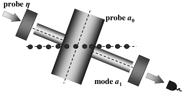
Figure 1: Setup. A lattice is illuminated by the transverse probe $a_{0}$ and probe through a mirror $\eta$. The photodetector measures photons of the cavity mode $a_{1}$ leaking out of the cavity. Due to the quantum back-action, the light measurement leads to the modification of the atomic quantum state.

We consider the model presented in Refs. PRL09 ; PRA09 . Using the approximation of macroscopic atomic ensemble with the large atom number, which is relevant for present experiments, will enable us to obtain a simple analytical solution in the next section.

We consider (cf. Fig. 1) $N$ ultracold atoms in an optical lattice of $M$ sites formed by strong off-resonant laser beams. A region of $K\leq M$ sites is also illuminated by a weak external probe, which is scattered into a cavity. Alternatively, this region is illuminated by the cavity field appearing due to the presence of the probe through the cavity mirror.

We use the open system approach for counting photons leaking the cavity of decay rate $\kappa$. When a photon is detected, the jump operator (the cavity photon annihilation operator $a_{1}$) is applied to the quantum state: $|\Psi_{c}(t)\rangle\rightarrow a_{1}|\Psi_{c}(t)\rangle$. Between the counts, the system evolves with a non-Hermitian Hamiltonian. Such an evolution gives a quantum trajectory for $|\Psi_{c}(t)\rangle$ conditioned on the detection of photons.

The expression for the initial motional state of atoms reads

$$|\Psi(0)\rangle=\sum_{q}c_{q}^{0}|q_{1},..,q_{M}\rangle,$$ (1)

which is a superposition of Fock states reflecting all possible classical configurations $q=\{q_{1},..,q_{M}\}$ of $N$ atoms at $M$ sites, where $q_{j}$ is the atom number at the site $j$. As we have shown in Refs. PRL09 ; PRA09 , the solution for conditional wave function takes physically transparent form, if the following approximations are used: atomic tunneling is much slower than light dynamics, the probe waves are in the coherent state, the first photon is detected after the time $1/\kappa$. The conditional state after the time $t$ and $m$ photocounts is given by the quantum superposition of solutions corresponding to the atomic Fock states in Eq. (1):

$$|\Psi_{c}(m,t)\rangle=\frac{1}{F(t)}\sum_{q}\alpha_{q}^{m}e^{\Phi_{q}(t)}c_{q}^{0}|q_{1},...,q_{M}\rangle|\alpha_{q}\rangle,$$ (2)

$$\alpha_{q}=\frac{\eta-iU_{10}a_{0}D^{q}_{10}}{i(U_{11}D^{q}_{11}-\Delta_{p})+\kappa},$$ (3)

$$\Phi_{q}(t)=-|\alpha_{q}|^{2}\kappa t+(\eta\alpha^{*}_{q}-iU_{10}a_{0}D^{q}_{10}\alpha^{*}_{q}-\text{c.c.})t/2,$$ (4)

where $\alpha_{q}$ is the cavity light amplitude corresponding to the classical configuration $q$. It is simply given by the Lorentz function (3) well-known from classical optics, where $a_{0}$ is the external probe amplitude, $\eta$ is the amplitude of the probe through a mirror; $U_{lm}=g_{l}g_{m}/\Delta_{a}$ ($l,m=0,1$), where $g_{1,0}$ are the atom-light coupling constants, $\Delta_{a}=\omega_{1}-\omega_{a}$ is the cavity-atom detuning; $\Delta_{p}=\omega_{p}-\omega_{1}$ is the probe-cavity detuning. $D^{q}_{lm}=\sum_{j=1}^{K}{u_{l}^{*}({\bf r}_{j})u_{m}({\bf r}_{j})q_{j}}$ are the probe-cavity coupling coefficient and dispersive frequency shift that sums contributions from all illuminated atoms with prefactors given by the light mode functions $u_{0,1}({\bf r})$. Except the prefactors associated with $m$ photodetections $\alpha_{q}^{m}$, the components of quantum superposition in Eq. (2) acquires the phases contained in $\Phi_{q}(t)$ (4). $F(t)$ is the normalization coefficient.

For several particular cases, the solution for the time-dependent probability distribution of atoms corresponding to the state (2) can be simplified further PRL09 ; PRA09 . If the probe, cavity, and lattice satisfy the condition of the diffraction maximum for light scattering, the probability to find the atom number $0<z<N$ in the lattice region of $K$ sites is given by

$$p(z,m,t)=z^{2m}e^{-z^{2}\tau}p_{0}(z)/\tilde{F}^{2},$$ (5)

$$\tilde{F}^{2}=\sum_{z}z^{2m}e^{-z^{2}\tau}p_{0}(z),$$

with $\tau=2|C|^{2}\kappa t$, $C=iU_{10}a_{0}/(i\Delta_{p}-\kappa)$, $p_{0}(z)$ is the initial distribution, and $\tilde{F}$ provides the normalization. The light amplitude corresponding to the atom number $z$ is $\alpha_{z}=Cz$.

If the condition of a diffraction minimum is satisfied, the probability to find the atom number difference between the odd and even sites in the lattice region of $K=M$ sites is given by the same Eq. (5), but with a different meaning of the statistical variable $-N<z<N$.

When the time progresses, both $m$ and $t$ increase with an essentially probabilistic relation between them. The Quantum Monte Carlo method, which establishes such a relation thus giving a quantum trajectory, consists in the following. The evolution is split into small time intervals $\delta t_{i}$. In each time step, the conditional photon number is calculated using the probability distribution (5):

$$\langle a^{\dagger}_{1}a_{1}\rangle_{c}(t)=|C|^{2}\sum_{z}z^{2}p(z,m,t),$$ (6)

which is proportional to the second moment of $p(z,m,t)$. The probability of the next, $(m+1)$th, photocount within this time interval $P_{m+1}=2\kappa\langle a^{\dagger}_{1}a_{1}\rangle_{c}\delta t_{i}$ is then compared with a random number $0<\epsilon_{i}<1$ generated in advance, thus, deciding whether the detection (if $2\kappa\langle a^{\dagger}_{1}a_{1}\rangle_{c}\delta t_{i}>\epsilon_{i}$) or no-count process (otherwise) has happened.

III Macroscopic quantum gases

In this section, we consider a case, where the initial atomic state is a macroscopic superfluid (SF) with the atom number $N\gg 1$. Note, that the total number of lattice sites $M$ and the number of sites illuminated $K$ can be any. Thus, the theory presented below can be applied for lattices with both low filling factors (e.g. one atom per lattice site in average) and very high filling factors (e.g. a BEC in a double-well potential).

We will start with the case of a diffraction minimum. As shown in Refs. PRL09 ; PRA09 , the probability function (5) to find the atom number difference $z$ between the odd and even sites shrinks to a doublet with the peaks at $z_{1,2}=\sqrt{m/\tau}$, which corresponds to the generation of the Schrödinger cat state.

For the SF state the probability to find the atom number at odd (or even) sites $\tilde{z}$ [$\tilde{z}=(z+N)/2$ as the atom number difference is $z$ and the total atom number is $N$] is given by the binomial distribution

$$p_{\text{SF}}(\tilde{z})=\frac{N!}{\tilde{z}!(N-\tilde{z})!}\left(\frac{Q}{M}\right)^{\tilde{z}}\left(1-\frac{Q}{M}\right)^{N-\tilde{z}},$$ (7)

where $Q$ is the number of odd (or even) sites. For even $M$, $Q=M/2$ and Eq. (7) simplifies. For a lattice with the large atom number $N\gg 1$, this binomial distribution can be approximated by a Gaussian function. Changing the variable as $z=2\tilde{z}-N$ we obtain the Gaussian function for the probability to find the atom number difference $z$:

$$p_{\text{SF}}(z)=\frac{1}{\sqrt{2\pi}\sigma}e^{-\frac{z^{2}}{2\sigma^{2}}}$$ (8)

with the zero mean $z$ and $\sigma=\sqrt{N}$ giving the full width at half maximum (FWHM) $2\sigma\sqrt{2\ln 2}$. The variance of the atom number difference in the SF state is $\sigma^{2}=N$.

For the large atom number, the summations in Eqs. (5) and (6) can be replaced by the integrals over all $-\infty<z<\infty$, which gives the following probability of the next photocount:

$$P_{m+1}=\frac{\int_{-\infty}^{\infty}{z^{2m+2}e^{-z^{2}\tau}e^{-\frac{z^{2}}{2\sigma^{2}}}dz}}{\int_{-\infty}^{\infty}{z^{2m}e^{-z^{2}\tau}e^{-\frac{z^{2}}{2\sigma^{2}}}dz}}\delta\tau_{i},$$ (9)

where $\delta\tau_{i}=2|C|^{2}\kappa\delta t_{i}$. Taking into account the following relation Gradstein :

$$\int_{0}^{\infty}{x^{2n}e^{-px^{2}}dx}=\frac{(2n-1)!!}{2(2p)^{n}}\sqrt{\frac{\pi}{p}},$$ (10)

the integrals can be calculated and the probability of the next photocount reads

$$P_{m+1}=\frac{m+1/2}{\tau+1/\sigma^{2}}\delta\tau_{i}.$$ (11)

Thus, we see that the Quantum Monte Carlo method, which is usually expected to be a basis for hard numerical simulations, has reduced to an extremely simple form. After splitting our time axis into intervals $\delta\tau_{i}$ and generating the random numbers $0<\epsilon_{i}<1$, one has simply to substitute the current time $\tau$ and the photocount number $m$ in the trivial algebraic expression (11) and realize if the next photocount happened or not. Proceeding this way one establishes the relation between the photocount number and time $m(\tau)$ at the quantum trajectory corresponding to the generated set of random numbers $\epsilon_{i}$. Knowing the relation between $m$ and $\tau$, one can calculate various conditional expectation values using Eq. (10) and the complementary expression

$$\int_{0}^{\infty}{x^{2n+1}e^{-px^{2}}dx}=\frac{n!}{2p^{n+1}}.$$ (12)

We now switch to the case of the light detection at the direction of a diffraction maximum. As shown in Refs. PRL09 ; PRA09 , in this case one measures the atom number $z$ in the lattice region of $K$ illuminated sites.

For the initial SF state the probability to find the atom number $z$ at the lattice region of $K$ sites is given by the binomial distribution

$$p_{\text{SF}}(z)=\frac{N!}{z!(N-z)!}\left(\frac{K}{M}\right)^{z}\left(1-\frac{K}{M}\right)^{N-z}.$$ (13)

For a lattice with the large atom number $N\gg 1$, it can be approximated as a Gaussian distribution

$$p_{\text{SF}}(z)=\frac{1}{\sqrt{2\pi}\sigma}e^{-\frac{(z-z_{0})^{2}}{2\sigma^{2}}}$$ (14)

with the mean atom number $z_{0}=NK/M$ and $\sigma=\sqrt{N(K/M)(1-K/M)}$ giving FWHM $2\sigma\sqrt{2\ln 2}$. The atom number variance in the SF state is $\sigma^{2}$.

Similarly to the case of a diffraction minimum, for the large atom number, the summations in Eqs. (5) and (6) can be replaced by the integrals over $-\infty<z<\infty$, which gives the following probability of the next photocount:

$$P_{m+1}=\frac{\int_{0}^{\infty}{z^{2m+2}e^{-z^{2}\tau}e^{-\frac{(z-z_{0})^{2}}{2\sigma^{2}}}dz}}{\int_{0}^{\infty}{z^{2m}e^{-z^{2}\tau}e^{-\frac{(z-z_{0})^{2}}{2\sigma^{2}}}dz}}\delta\tau_{i}.$$ (15)

Taking into account the following relation Gradstein :

$$\int_{-\infty}^{\infty}{x^{n}e^{-px^{2}+2qx}dx}=\frac{1}{2^{n-1}p}\sqrt{\frac{\pi}{p}}\frac{d^{n-1}}{dq^{n-1}}\left(qe^{\frac{q^{2}}{p}}\right)$$ (16)

$$=n!e^{\frac{q^{2}}{p}}\sqrt{\frac{\pi}{p}}\left(\frac{q}{p}\right)^{n}\sum_{k=0}^{E(n/2)}\frac{1}{(n-2k)!k!}\left(\frac{p}{4q^{2}}\right)^{k},$$

where $E(n/2)$ is the integer part of $n/2$, the integrals can be calculated and the probability of the next photocount reads

$$P_{m+1}=(2m+1)(2m+2)a^{2}\sum_{k=0}^{m+1}\frac{b^{k}}{(2m+2-2k)!k!}/\sum_{k=0}^{m}\frac{b^{k}}{(2m-2k)!k!},$$ (17)

where the parameters are

$$a=\frac{z_{0}}{2\sigma^{2}(\tau+1/(2\sigma^{2}))}=\frac{1}{2(1-K/M)(\tau+1/(2\sigma^{2}))},$$

$$b=\frac{\tau+1/(2\sigma^{2})}{z_{0}^{2}}\sigma^{4}=(\tau+1/(2\sigma^{2}))\left(1-\frac{K}{M}\right)^{2}.$$

Expression (17) is more complicated than Eq. (11) for the diffraction minimum. However, it is also very simple as it includes only summation over the photocount number. Thus, we were able to replace the summation over the atom number, which can rich the values of $N=10^{5}$, and even the numerical integration over the atom number. For the far off-resonant interaction considered here, the number of photocounts $m$ will be many orders of magnitude less than the atom number. So, the sum in Eq. (17) will contain only a small number of terms.

IV Purity of the final state

As shown in Ref. PRA09 , under some conditions, the entangled light-matter state can collapse to a macroscopic superposition state, which has a form

$$|\Psi_{c}\rangle=\frac{1}{\sqrt{2}}[e^{i\gamma}|z_{1}\rangle|\alpha_{z_{1}}\rangle+e^{-i\gamma}|z_{2}\rangle|\alpha_{z_{2}}\rangle],$$ (18)

where $\gamma$ is some phase, $|z_{1,2}\rangle$ are the atomic Fock states with precisely known atom numbers $z_{1}$ and $z_{2}$. $|\alpha_{z_{1,2}}\rangle$ are the corresponding coherent states of light such that the light amplitudes have equal absolute values, but opposite phases: $\alpha_{z_{1}}=|\alpha_{z_{1}}|\exp{(i\varphi)}$ and $\alpha_{z_{2}}=|\alpha_{z_{1}}|\exp{(-i\varphi)}$.

Expression (18) gives a macroscopic superposition state, where light and atoms are entangled. One possibility to disentangle them is to switch off the probe and count the photons leaking out of the cavity. In this case both $|\alpha_{z_{1}}\rangle$ and $|\alpha_{z_{2}}\rangle$ will approach the vacuum state $|0\rangle$ and the light and matter will factorize. The difficulty of such a method consists in the necessity to count almost all photons to get finally an atomic state of high purity PRA09 . In this paper, we analyze the state obtained by tracing out the light field directly in Eq. (18), without waiting for photon leakage. This corresponds to a scheme, where the measurement of light is not performed.

The trace over the light variables can be calculated using the photon Fock basis, in which the coherent light states read

$$|\alpha_{z_{1,2}}\rangle=e^{-|\alpha_{z_{1}}|^{2}/2}\sum_{n=0}^{\infty}\frac{|\alpha_{z_{1}}|^{n}e^{\pm n\varphi}}{\sqrt{n!}}|n>.$$ (19)

The density matrix of the state after tracing out the light is $\rho=\sum_{n=0}^{\infty}\langle n|\Psi_{c}\rangle\langle\Psi_{c}|n\rangle$. Using the expression

$$\sum_{n=0}^{\infty}\frac{|\alpha_{z_{1}}|^{2n}}{n!}e^{-|\alpha_{z_{1}}|^{2}}e^{-2in\varphi}=e^{|\alpha_{z_{1}}|^{2}(e^{-2i\varphi}-1)},$$ (20)

the density matrix takes the form

$$\rho=\frac{1}{2}\left(|z_{1}\rangle\langle z_{1}|+|z_{2}\rangle\langle z_{2}|+e^{|\alpha_{z_{1}}|^{2}(e^{2i\varphi}-1)}e^{2i\gamma}|z_{1}\rangle\langle z_{2}|+e^{|\alpha_{z_{1}}|^{2}(e^{-2i\varphi}-1)}e^{-2i\gamma}|z_{2}\rangle\langle z_{1}|\right)$$ (21)

The quantity characterizing how close is a mixture state to a pure state is the so-called purity: $P=\text{Tr}(\rho^{2})$. For a pure state it is maximal and equal to 1, while for a maximally mixed state it is minimal and equal to $1/2$ (in our case of the two-component states). The purity of the state (21) is given by

$$P=\frac{1}{2}\left(1+e^{-4|\alpha_{z_{1}}|^{2}\sin^{2}\varphi}\right).$$ (22)

The purity depends on the amplitude of the coherent light states in Eq. (18) and the phase difference between them. In a trivial case, where two coherent states are indistinguishable ($\varphi=0$), the purity is maximal, $p=1$, and the state is pure (however, in this case, $z_{1}=z_{2}$ and the state is not a macroscopically entangled one). In non-trivial cases, where the coherent states differ by the phase $2\varphi$, the purity decreases with increase of the light amplitude and phase difference between them. One can estimate the minimal possible purity as follows. In a coherent state, the uncertainty of the $X$-quadrature is $1/2$. Thus, two coherent states can be well distinguished, if $|\alpha_{z_{1}}|\sin\varphi>1/4$. Substituting the minimal value 1/4 in Eq. (22), one sees that the maximal purity can reach 0.89, which is a rather high value.

V Conclusions

We have considered the quantum measurement of light scattered from an ultracold quantum gas. Due to the light-matter entanglement, the back-action of light measurement modifies the atomic state as well. We applied our theory developed in Refs. PRL09 ; PRA09 for the case of a macroscopic BEC with a large atom number. We have shown that the Quantum Monte Carlo simulation method gets very simple in that case and the calculations can be carried out even analytically. The purity of the macroscopic superposition atomic state was analyzed and shown to be able to reach the high values.

References

- (1) F. Brennecke, T. Donner, S. Ritter, T. Bourdel, M. Kohl, and T. Esslinger, Nature 450, 268 (2007).
- (2) Y. Colombe, T. Steinmetz, G. Dubois, F. Linke, D. Hunger, and J. Reichel, Nature 450, 272 (2007).
- (3) S. Slama, S. Bux, G. Krenz, C. Zimmermann, and Ph. W. Courteille, Phys. Rev. Lett. 98, 053603 (2007).
- (4) S. Ritter, F. Brennecke, C. Guerlin, K. Baumann, T. Donner, T. Esslinger, Appl. Phys. B 95, 213 (2009).
- (5) F. Brennecke, S. Ritter, T. Donner, T. Esslinger, Science 322, 235 (2008).
- (6) C. Maschler and H. Ritsch, Phys. Rev. Lett. 95, 260401 (2005).
- (7) I. B. Mekhov, C. Maschler, and H. Ritsch, Nature Phys. 3, 319 (2007).
- (8) I. B. Mekhov, C. Maschler, and H. Ritsch, Phys. Rev. Lett. 98, 100402 (2007).
- (9) I. B. Mekhov, C. Maschler, and H. Ritsch, Phys. Rev. A 76, 053618 (2007).
- (10) C. Maschler, I. B. Mekhov, and H. Ritsch, Eur. Phys. J. D 46, 545 (2008).
- (11) I. B. Mekhov and H. Ritsch, Phys. Rev. Lett. 102, 020403 (2009).
- (12) I. B. Mekhov, and H. Ritsch, Phys. Rev. A 80, 013604 (2009).
- (13) I. B. Mekhov and H. Ritsch, Laser Phys. 19, 610 (2009).
- (14) A. Vukics, W. Niedenzu, and H. Ritsch, Phys. Rev. A 79, 013828 (2009).
- (15) H. Zoubi and H. Ritsch, arXiv:0902.2638.
- (16) W. Chen, D. Meiser, and P. Meystre, Phys. Rev. A 75, 023812 (2007).
- (17) J. Larson, B. Damski, G. Morigi, and M. Lewenstein, Phys. Rev. Lett. 100, 050401 (2008).
- (18) J. Larson, S. Fernandez-Vidal, G. Morigi, and M. Lewenstein, New J. Phys. 10, 045002 (2008).
- (19) K. Eckert, O. Romero-Isart, M. Rodriguez, M. Lewenstein, E. Polzik, and A. Sanpera, Nature Phys. 4, 50 (2008).
- (20) A. B. Bhattacherjee, Opt. Commun. 281, 3004 (2008).
- (21) J. M. Zhang, W. M. Liu, and D. L. Zhou, Phys. Rev. A 77, 033620 (2008).
- (22) J. M. Zhang, W. M. Liu, and D. L. Zhou, Phys. Rev. A 78, 043618 (2008).
- (23) J. Ye, J. Zhang, W. Liu, K. Zhang, Y. Li, Z.-Y. Ou, and W. Zhang, arXiv:0812.4077.
- (24) A. B. Bhattacherjee, arXiv:0906.2624.
- (25) K. Lakomy, Z. Idziaszek, and M. Trippenbach, arXiv:0904.2927.
- (26) L. Guo, S. Chen, B. Frigan, L. You, and Y. Zhang, Phys. Rev. A 79, 013630 (2009).
- (27) W. Chen and P. Meystre, Phys. Rev. A 79, 043801 (2009);
- (28) W. Chen, K. Zhang, D. S. Goldbaum, M. Bhattacharya, and P. Meystre, Phys. Rev. A 80, 011801(R) (2009).
- (29) K. Zhang, W. Chen, P. Meystre, arXiv:0906.4143.
- (30) J. M. Zhang, S. Cui, H. Jing, D. L. Zhou, and W. M. Liu, arXiv:0907.1200.
- (31) S. Rist, C. Menotti, and G. Morigi, arXiv:0904.0915.
- (32) L. S. Gradstein and I. M. Ryzhik, Tables of Integrals, Series and Products (Academic Press, 1980).