Intrinsic Spin Hall Effect in Non-Cubic Crystals

Abstract

We study the dependence of the intrinsic spin Hall effect on the crystal symmetry and geometry of experiment. The spin current is obtained and the Hall voltage caused by the polarization of the electron spins is computed. The unique dependence of the effect on the crystal symmetry permits the choice of geometry in which the spin Hall effect can be unambiguously distinguished from the effects due to the orbital motion of charge carriers and due to the magnetic field generated by the transport current.

The spin Hall effect consists of opposite “Hall” currents for charge carriers with opposite spin polarizations. Remarkably, no magnetic field is needed for the electrons with spin up and spin down to veer in opposite directions. The effect was initially observed in GaAs strips by Kato et al. via Kerr signal Kato , and by Wunderlich et al. via polarization of light emitted at the recombination of spin-polarized electron-hole pairs Wunderlich . When numbers of spin-up and spin-down electrons are equal, no net electric current across the strip is generated by the spin Hall effect. If, however, the electrons are polarized due to, e.g., injection from a ferromagnet DasSarma , then the numbers of electrons veering left and right are different and a Hall voltage is produced. Valenzuela and Tinkham used this effect to measure the spin Hall conductivity in the aluminum strip Tinkham .

Dyakonov and Perel DP were apparently the first to suggest that scattering of charge carriers by unpolarized impurities in semiconductors can lead to the spin polarization of the sample boundaries. Their suggestion was based upon a similar effect in atomic physics known as Mott scattering Mott . When a relativistic electron passes at a speed ${\bf v}$ through an atom, the partially unscreened electric field of the nucleus, ${\bf E}$, creates the magnetic field ${\bf B}={\bf E}\times{\bf v}/c$ in the coordinate frame of the electron. This field partially polarizes the electron spin in the direction that is opposite for the electrons passing the nucleus on the right and on the left. Consequently, one can achieve a spatial separation of spin-up and spin-down electrons when unpolarized electron beam passes through unpolarized atomic target.

A number of microscopic models have been developed that extended these ideas to solids. Various “extrinsic” (due to impurities) and “intrinsic” (impurity-free) mechanisms have been studied with the aim to explain quantitatively the spin Hall effect in non-magnetic conductors Rashba , as well as to explain the anomalous Hall effect in magnetic materials anomalous . Most of the existing theoretical models are based upon the Boltzmann-type kinetic equation that describes spin and charge transport under certain assumptions about the collision integral. There is also a vast amount of numerical work of disordered systems in lattices of finite size. So far these works have not offered any universal description of the spin Hall effect. Instead a variety of different spin Hall effects (spin precession, side jump, skew scattering) that are specific to the model of spin-orbit interaction, nature of scatterers, band structure, boundary effects, etc. has been proposed. A simple single-electron picture of the intrinsic spin Hall effect, similar to the treatment of the conventional Hall effect within Drude model, has been suggested in Ref. EC, . In this picture the Mott scattering of the transport current by the crystal field appears naturally within the framework of the Aharonov-Casher effect AC . The parameter-free expression for the spin Hall conductivity was obtained for cubic crystals in good agreement with experiments. In this paper we will extend the treatment of Ref. EC, to non-cubic crystals. Straightforward experiments will be suggested that can test our predictions.

Our approach is based upon the general form of the one-electron Hamiltonian that contains spin-orbit interaction to $1/c^{2}$ Drell :

$${\cal{H}}=\frac{{\bf p}^{2}}{2m}+U({\bf r})+\frac{\hbar}{4m^{2}c^{2}}{\bm{\sigma}}\cdot\left({\bm{\nabla}}U\times{\bf p}\right)\,.$$ (1)

It is exactly this Hamiltonian, with $U({\bf r})$ being the electric potential of the atom, that is responsible for the Mott scattering of electrons in the atomic physics. In a solid, $U({\bf r})$ is the electrostatic crystal potential felt by a charge carrier. For certainty we will speak about electrons but the model will equally apply to holes. With an accuracy to $1/c^{2}$ Hamiltonian (1) is mathematically equivalent to AC

$${\cal{H}}=\frac{1}{2m}\left({\bf p}-\frac{e}{c}{\bf A}_{\sigma}\right)^{2}+U({\bf r})$$ (2)

where $e<0$ is the charge of electron and EC

$${\bf A}_{\sigma}\equiv-\frac{\hbar}{4emc}\left({\bm{\sigma}}\times{\bm{\nabla}}U\right)\,.$$ (3)

(We have used the mathematical fact that the action of the operator ${\bf p}$ on ${\bf A}_{\sigma}$ is zero, $\epsilon_{ijk}\sigma_{j}\nabla_{i}\nabla_{k}U=0$.) Consequently, the orbital motion of electrons is affected by the fictitious spin-dependent magnetic field:

$${\bf B}_{\sigma}={\bm{\nabla}}\times{\bf A}_{\sigma}=-\frac{\hbar}{4emc}\,\left[{\bm{\nabla}}\times\left({\bm{\sigma}}\times{\bm{\nabla}}U\right)\right]\,.$$ (4)

This fictitious field produces the same effect on the orbital motion of electrons as the real magnetic field does in the conventional Hall effect, but with the Hall currents having opposite directions for electrons with opposite spin polarizations. The spin-dependent Lorentz force, ${\bf F}_{L\sigma}=-(e/c)({\bf v}\times{\bf B}_{\sigma})$, gives rise to the fictitious spin-dependent Hall electric field,

$${\bf E}_{H\sigma}=R_{H}\left({\bf B}_{\sigma}\times{\bf j}_{0}\right)\,,$$ (5)

where ${\bf j}_{0}=en{\bf v}_{0}$ is the transport current expressed through the concentration $n$ and drift velocity ${\bf v}_{0}$ of the electrons, and $R_{H}=-1/(nec)$ is the Hall constant. If the electrons are polarized, the spin average of Eq. (4) gives rise to the effective magnetic field,

$${\bf B}_{eff}=-\frac{\hbar}{4emc}\,\langle{\bm{\nabla}}\times\left({\bm{\xi}}\times{\bm{\nabla}}U\right)\rangle\,,$$ (6)

and to the measurable Hall electric field:

$${\bf E}_{H}=R_{H}\left({\bf B}_{eff}\times{\bf j}_{0}\right)\,.$$ (7)

In these formulas $0<\xi<1$ is the polarization of the electrons and $\langle...\rangle$ denotes the space average. If polarized electrons are injected from, e.g., a magnetic metal, ${\bf j}_{0}$ describes the flow of the injected electrons.

In the presence of the real magnetic field ${\bf B}$, Eq. (2) should be replaced by

$${\cal{H}}=\frac{1}{2m}\left({\bf p}-\frac{e}{c}{\bf A}-\frac{e}{c}{\bf A}_{\sigma}\right)^{2}+U({\bf r})+\frac{g}{2}\mu_{B}{\bm{\sigma}}\cdot{\bf B}\,,$$ (8)

where ${\bf A}=({\bf B}\times{\bf r})/2$, $g$ is the gyromagnetic factor, and $\mu_{B}$ is the Bohr magneton. Since the definition of ${\bf A}_{\sigma}$, Eq. (3), already contains $1/c$, the cross-term proportional to ${\bf A}\cdot{\bf A}_{\sigma}$ in Eq. (8) has the order $1/c^{3}$. Within the non-relativistic approximation of Eq. (1), that has accuracy to $1/c^{2}$, such a cross-term must be omitted. Consequently, in the non-relativistic theory the conventional Hall effect and the spin Hall effect are totally independent. For that reason and in order to emphasize the consequences of the spin Hall effect, we are considering below the case of ${\bf B}=0$.

When writing down Eq. (5) and Eq. (7) we made an assumption that $\langle{\bf v}\times{\bf B}_{\sigma}\rangle=\langle{\bf v}\rangle\times\langle{\bf B}_{\sigma}\rangle$. Some justification of this assumption follows from the fact that the trajectory of the charge carrier does not correlate strongly with the quadrupole component of the crystal electric field contained in the expression for ${\bf B}_{\sigma}$. Another argument is based upon symmetry. Indeed, the only reason for $\langle{\bf F}_{L\sigma}\rangle$ to be different from zero would be ${\bf v}_{0}\equiv\langle{\bf v}\rangle\neq 0$. Consequently, $\langle{\bf F}_{L\sigma}\rangle$ should be first order on ${\bf v}_{0}$. Being perpendicular to the velocity, the force ${\bf F}_{L\sigma}$ does not do mechanical work on the charge. Neither should $\langle{\bf F}_{L\sigma}\rangle$ with respect to the drift motion of the charges, rendering the form $\langle{\bf F}_{L\sigma}\rangle=-(e/c)({\bf v}_{0}\times\tilde{\bf B})$. It is natural to identify $\tilde{\bf B}$ with ${\bf B}_{eff}$ of Eq. (6).

To show that space averaging in Eq. (6) produces a non-zero result, one needs to compute $\langle\nabla_{i}\nabla_{j}U({\bf r})\rangle$. Experiments performed to date have been done in cubic semiconductors and in aluminum that is also cubic Kato ; Wunderlich ; Tinkham . For a cubic lattice

$$\langle{\bm{\nabla}}_{i}{\bm{\nabla}}_{j}U\rangle=C\delta_{ij}$$ (9)

due to the cubic symmetry alone, with $C$ being a constant. This constant can be found from the Laplace equation:

$$C\equiv\frac{1}{3}\langle{\bm{\nabla}}^{2}U({\bf r})\rangle=-\frac{4\pi}{3}e\langle\rho({\bf r})\rangle\,,$$ (10)

where $\rho({\bf r})$ is the charge density that creates $U({\bf r})$. To make the right choice for $\rho({\bf r})$, we notice that the spin-orbit interaction becomes larger as the electron passes closer to the nucleus. Similar to the Mott scattering by individual atoms, the electric neutrality of the crystal as a whole Kravchenko is irrelevant for our problem; the distances that matter are the ones where the screening of the electric charge of the nuclei is not complete EC-reply . Consequently, the spatial average in Eq. (6) must be over short distances. Due to the periodicity of the crystal it can be computed over the unit cell. In that sense our symmetry argument for the cubic lattice and other lattices studied below is similar to the argument used to compute the crystal field (magnetocrystalline anisotropy) in magnetically ordered crystals lectures .

In line with the conventional approach to solids AM , we choose $U({\bf r})$ as the potential formed by a cubic lattice of ions of charge $-Ze>0$. Then $\langle\rho\rangle=-Zen_{0}=-en$ where $n_{0}$ and $n=Zn_{0}$ are concentrations of ions and conduction electrons, respectively. This gives $C=4\pi e^{2}n/3$ EC . Those who find this argument too simplistic may want to compare it with the approach developed by Hirsch Hirsch-99 . In a model that replaces moving spins with stationary electric dipoles Hirsch computed the same average over a cubic lattice of charges numerically. To nine decimal places his result coincides with ours up to a factor of $2$ that can be traced to the difference in the expression for the fictitious magnetic field Hirsch-sign . Note that in a microscopic model the right-hand side of Eq. (10) contains a sum over delta-functions. It is therefore likely that at the microscopic level the spin Hall effect originates from the singularity of the Coulomb potential. Since our model does not treat the screening effects rigorously and does not take into account the interaction between the electrons, our result for $C$ can only be valid up to a factor of order unity.

Substitution of Eq. (9) into Eq. (6) gives

$${\bf B}_{eff}=C\frac{\mu_{B}}{e^{2}}{\bm{\xi}}=\frac{4\pi}{3}n\mu_{B}{\bm{\xi}}\,,$$ (11)

which provides the Hall field

$${\bf E}_{H}=-\frac{2\pi\hbar}{3mc^{2}}\left({\bm{\xi}}\times{\bf j}_{0}\right)\,.$$ (12)

Note that this formula does not contain any dependence on the concentration of charge carriers. Only the knowledge of ${\bm{\xi}}$ and ${\bf j}_{0}$ are needed to compute the Hall electric field. This allows easy analysis of experiments with polarized electrons in cubic conductors. One can see a potential problem, however, with interpreting the Hall voltage in Eq. (12) as a spin Hall effect. Indeed, the effective field in Eq. (11) equals the magnetic field that the polarized electrons would produce in a spherically shaped body; with $4\pi/3$ being the demagnetizing factor. The magnetic field due to polarization of electron spins in the actual sample should be different by a factor of order unity. Nevertheless, given the experimental uncertainties, it may be difficult to practically distinguish the spin Hall effect described by Eq. (12) from the conventional Hall effect due to the magnetic field produced by the electron polarization.

In fact, the above-mentioned controversy is a consequence of the cubic symmetry. Indeed, in the conventional Hall effect only the orbital motion of the electron matters, the electron spin is irrelevant. On the contrary, the spin Hall effect arises from the spin-orbit term in the Hamiltonian. Consequently, there must be a clear way to distinguish between the two effects. As we shall see below, the non-cubic crystals present such a possibility. Consider, e.g., a tetragonal crystal with ${\bf n}$ being the unit vector in the direction of the $c$-axis. By symmetry, Eq. (9) should be now replaced with ($a=b$)

$$\langle{\bm{\nabla}}_{i}{\bm{\nabla}}_{j}U\rangle=C[k_{a}\delta_{ij}+(k_{c}-k_{a})n_{i}n_{j}]\,,$$ (13)

where $k_{a}\neq k_{c}$ are factors of order unity. Working out the cross-products in Eq. (6) one obtains

$${\bf B}_{eff}=C\frac{\mu_{B}}{2e^{2}}\left[(k_{a}+k_{c}){\bm{\xi}}+(k_{a}-k_{c})({\bf n}\cdot{\bm{\xi}}){\bf n}\right]\,.$$ (14)

The new feature is the component of the effective field along the tetragonal axis. (Notice the analogy with the magnetic anisotropy field in a magnetically ordered uniaxial crystal lectures .)

Substitution of Eq. (14) into Eq. (7) gives

$${\bf E}_{H} = -\frac{\pi\hbar}{3mc^{2}}[(k_{a}+k_{c})({\bm{\xi}}\times{\bf j}_{0})$$ (15)

$$+ (k_{a}-k_{c})({\bf n}\cdot{\bm{\xi}})({\bf n}\times{\bf j}_{0})]\,.$$

This formula must be also correct for a hexagonal crystal, with ${\bf n}$ along the hexagonal axis. Its remarkable property is that due to the second term the Hall voltage can be produced in the sample even when the electrons are polarized along the direction of the transport current. This would be a clear manifestation of the Hall effect due to the spin, in contrast with the ordinary Hall effect due to the conventional spin-independent Lorentz force on the transport current. One possible geometry of the experiment is shown in Fig. 1.

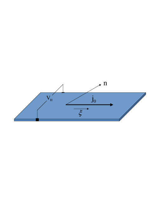
Figure 1: Color online: Geometry of the proposed experiment. The crystal anisotropy axis is at an angle with the film. Due to the spin Hall effect the Hall voltage appears even when the electron spins are polarized along the transport current.

Until now we have studied the spin Hall effect in a system of partially polarized electrons. Alternatively, one can study the spin currents that would polarize the boundaries of the sample in the absence of the polarization in the bulk. In fact, this is how the spin Hall effect was initially observed Kato ; Wunderlich . The spin current is defined Rashba as the one-particle expectation value of

$$j_{ik}=\frac{1}{2}en(\sigma_{i}v_{k}+v_{k}\sigma_{i})\,,$$ (16)

In general it is not conserved. However, due to the relativistic smallness of spin-orbit interaction the reversal of the electron spin occurs only in a small fraction of scattering events. Consequently, in a small sample at low temperature the charge carriers typically reach the boundary of the sample before scattering reverses their spins. In this case Eq. (16) provides a useful concept for the study of the spin accumulation at the boundaries.

Since Eq. (16) contains Pauli matrices, the non-zero expectation value of $j_{ik}$ is provided by the spin-dependent part of the velocity operator. The latter is given by EC

$${\bf v}_{\sigma}=\frac{e\tau}{m}{\bf E}_{H\sigma}\,,$$ (17)

where $\tau$ is the scattering time. Consider, e.g., an orthorhombic crystal. By symmetry the principal axes of the second-rank tensor $\langle{\bm{\nabla}}_{i}{\bm{\nabla}}_{j}U\rangle$ should be directed along the $a,b,c$ axes of the crystal. Choosing the axes of the coordinate frame along the crystal axes, we present $\langle{\bm{\nabla}}_{i}{\bm{\nabla}}_{j}U\rangle$ in a diagonal form:

$$\langle{\bm{\nabla}}_{i}{\bm{\nabla}}_{j}U\rangle=Ck_{i}\delta_{ij}\,,$$ (18)

with $k_{x,y,z}$ being generally unequal factors of order unity. Substitution of Eq. (18) into Eq. (4) then gives

$$B_{\sigma i}=C\frac{\mu_{B}}{2e^{2}}\sigma_{i}(k_{x}+k_{y}+k_{z}-k_{i})\,.$$ (19)

Finally, with the help of equations (5), (16), (17), and (19), one obtains

$$j_{ik}=\frac{\pi\hbar\sigma_{0}}{3mc^{2}}\epsilon_{ikl}(k_{x}+k_{y}+k_{z}-k_{i})j_{0l}\,,$$ (20)

where $\sigma_{0}=e^{2}n\tau/m$ is the usual charge conductivity. According to this equation, the strength of the spin current as compared to the charge current is determined by the factor $\hbar\sigma_{0}/(mc^{2})$ which also determines the ratio of spin Hall and charge conductivities EC . For good metals at low temperature this ratio can be of order $10^{-4}$.

For a cubic crystal $k_{x}=k_{y}=k_{z}=1$ and Eq. (20) reduces to the expression

$$j_{ik}=\frac{2\pi\hbar\sigma_{0}}{3mc^{2}}\,\epsilon_{ikl}j_{0l}$$ (21)

which is independent of the orientation of the crystal lattice with respect to the transport current. This may present a problem for distinguishing the polarization of the sample boundaries generated by the spin Hall effect from the spin polarization generated by the Zeeman effect due to the magnetic field of the current. This controversy can be resolved by studying the spin Hall effect in a non-cubic crystal. Consider, e.g., two geometrically identical conducting strips, one cut along the $aa$-plane and the other cut along the $ac$-plane of a tetragonal crystal, with the $z$-axis being perpendicular to the plane of the strip and the transport current being along the $y$-axis. It is easy to see from Eq. (20) that the spin current $j_{zx}=[{\pi\hbar\sigma_{0}}/(3mc^{2})](k_{x}+k_{y})j_{0}$, describing the flow of $\sigma_{z}$ along the $x$-axis, is different for the two strips. The ratio of these spin currents for the same value of the transport current is given by $j_{zx}(aa)/j_{zx}(ac)=2k_{a}/(k_{a}+k_{c})\neq 1$. Consequently, the spin polarizations of the boundaries generated by the spin Hall effect will also be different for the two strips, while polarizations generated by the Zeeman effect due to the magnetic field of the transport current will be the same.

In Conclusion, we have studied the intrinsic spin Hall effect in non-cubic crystals. The unique dependence of the effect on the crystal symmetry permits geometry of experiment in which the spin Hall effect can be unambiguously distinguished from the effects caused by the orbital motion of charge carriers and by the magnetic field of the transport current.

The author thanks David Awschalom for bringing his attention to recent experimental papers on spin Hall effect in non-cubic crystals Awschalom . This work has been supported by the Department of Energy through Grant No. DE-FG02-93ER45487.

References

- (1) Y. K. Kato, R. C. Myers, A. C. Gossard, and D. D. Awschalom, Science 306, 1910 (2004).
- (2) J. Wunderlich, B. Kaestner, J. Sinova, T. Jungwirth, Phys. Rev. Lett. 94, 047204 (2005).
- (3) I. Z̆utić, J. Fabian, and S. Das Sarma, Rev. Mod. Phys. 76, 323 (2004).
- (4) S. O. Valenzuela and M. Tinkham, Nature 442, 176 (2006).
- (5) M. I. Dyakonov and V. I. Perel, JETP Lett. 13, 467 (1971); Phys. Lett. A 35, 459 (1971).
- (6) N. F. Mott, Proc. R. Soc. London A 124, 425 (1929).
- (7) H.-A. Engel, E. I. Rashba, and B. I. Halperin, Theory of Spin Hall Effects in Semiconductors, in Handbook of Magnetism and Advanced Magnetic Materials, pp. 2858-2877 (H. Kronmüller and S. Parkin - editors, John Wiley & Sons Ltd, Chichester, United Kingdom, 2007).
- (8) See for review: N. A. Sinitsyn, J. Phys.: Cond. Matt. 20, 023201 (2008); N. Nagaosa, J. Sinova, S. Onoda, A. H. MacDonald, N. P. Ong, arXiv:cond-mat/0904.4154, to appear in Rev. Mod. Phys.
- (9) E. M. Chudnovsky, Phys. Rev. Lett. 99, 206601 (2007).
- (10) Y. Aharonov and A. Casher, Phys. Rev. Lett. 53, 319 (1984).
- (11) J. D. Bjorken and S. D. Drell, Relativistic Quantum Mechanics (McGraw-Hill, 1965).
- (12) See, e.g., N. W. Ashcroft and N. D. Mermin, Solid State Physics, Chapter 8, (Holt, Rinehart, and Winston, New York, 1976).
- (13) V. Ya. Kravchenko, Phys. Rev. Lett. 100, 199703 (2008).
- (14) E. M. Chudnovsky, Phys. Rev. Lett. 100, 199704 (2008).
- (15) See, e.g., E. M. Chudnovsky and J. Tejada, Lectures on Magnetism (Rinton Press, Princeton, NJ, 2006).
- (16) J. E. Hirsch, Phys. Rev. B 60, 14787 (1999).
- (17) J. E. Hirsch, Ann. Phys. (Berlin) 17, 380 (2008). Notice the wrong sign of the vector-potential term in the Hamiltonian, Eq. (108a), that follows from the heuristic model of Hirsch.
- (18) V. Sih, R. C. Myers, Y. K. Kato, W. H. Lau, A. C. Gossard, D. D. Awschalom, Nature Phys. 1, 31 (2005); N. P. Stern, S. Ghosh, G. Xiang, M. Zhu, N. Samarth, D. D. Awschalom, Phys. Rev. Lett. 97, 126603 (2006); W. F. Koehl, M. H. Wong, C. Poblenz, B. Swenson, U. K. Mishra, J. S. Speck, D. D. Awschalom, Appl. Phys. Lett. 95, 072110 (2009).