Degree Correlations in a Dynamically Generated Model Food Web

Abstract

We explore aspects of the community structures generated by a simple predator-prey model of biological coevolution, using large-scale kinetic Monte Carlo simulations. The model accounts for interspecies and intraspecies competition for resources, as well as adaptive foraging behavior. It produces a metastable low-diversity phase and a stable high-diversity phase. The structures and joint indegree-outdegree distributions of the food webs generated in the latter phase are discussed.

I Introduction and Model

Biological evolution and ecology involve nonlinear interactions between large numbers of units and have recently become popular topics among statistical and computational physicists DROS01 . However, many models used by physicists are unrealistic to the extent of attracting little attention from biologists. Here, we introduce a somewhat more realistic model of the dynamics of a predator-prey system and explore some aspects of the resulting food-web structures.

Recently, we developed simplified models of biological macroevolution RIKV03 ; RIKV06 , in which the reproduction rates in an individual-based population dynamics with nonoverlapping generations provide the mechanism for selection between several interacting species. New species enter the community through point mutations in a haploid, binary “genome” of length $L$. The potential species are identified by the index $I\in[0,2^{L}-1]$. (Typically, only $\mathcal{N}(t)\ll 2^{L}$ species are present in the community at any time $t$.) At the end of each generation, each individual of species $I$ gives birth to a fixed number $F$ of offspring with probability $P_{I}$ before dying, or dies without offspring with probability $(1-P_{I})$. Each offspring may mutate into a different species with a small probability $\mu$. Mutation consists in flipping a randomly chosen bit in the genome.

Here, we consider a model with modified population dynamics that include competition between different predators that prey on the same species, as well as a satiation effect for predators with abundant prey. Consistent with our previous work RIKV06 , the central quantity of the model is an antisymmetric interaction matrix $\bf M$ representing predator-prey interactions. Thus, $M_{IJ}>0$ and $M_{JI}<0$ means that $I$ is a predator and $J$ its prey, and vice versa. The elements of the upper triangle of $\bf M$ are drawn randomly from a symmetric distribution over $[-1,+1]$ and kept constant during the whole simulation (quenched randomness). A constant, $R>0$, represents an external resource. The ability of species $I$ to utilize $R$ is $\eta_{I}$, which with probability $c_{\rm prod}\ll 1$ is chosen to be a random number uniform on $(0,+1]$ (i.e., $c_{\rm prod}$ is the proportion of potential producer species). Species with $\eta_{I}=0$ are consumers. The population size of species $I$ is $n_{I}$.

Interspecies competition is modeled by defining the number of individuals of species $J$ that are available as prey for $I$, corrected for competition from other predator species, as

$$\hat{n}_{IJ}=\frac{n_{I}M_{IJ}}{\sum_{L}^{{\rm pred}(J)}n_{L}M_{LJ}}n_{J}\;,$$ (1)

where $\sum_{L}^{{\rm pred}(J)}$ runs over all $L$ such that $M_{LJ}>0$. Thus, $\sum_{I}^{{\rm pred}(J)}\hat{n}_{IJ}=n_{J}$. Analogously, we define the competition-adjusted external resources available to a producer species $I$ as $\hat{R}_{I}=R{n_{I}\eta_{I}}/{\sum_{L}n_{L}\eta_{L}}$. With these definitions, the total, competition-adjusted resources available to species $I$ are

$$\hat{S}_{I}=\eta_{I}\hat{R}_{I}+\sum_{J}^{{\rm prey}(I)}M_{IJ}\hat{n}_{IJ}\;,$$ (2)

where $\sum_{J}^{{\rm prey}(I)}$ runs over all $J$ such that $M_{IJ}>0$.

The functional response of species $I$ with respect to $J$, $\Phi_{IJ}$, is the rate at which an individual of species $I$ consumes individuals of $J$ DROS01B ; KREB01 . For ecosystems consisting of a single pair of predator and prey, or a simple chain from a bottom-level producer through intermediate species to a top predator, the most common forms of functional response are due to Holling KREB01 . For more complicated food webs, several functional forms have been proposed recently, DROS01B ; SKAL01 ; DROS04 ; MART06 but there is as yet no agreement about a standard form. Here, we model intraspecies competition by a ratio-dependent RESI95 Holling Type II KREB01 form due to Getz GETZ84 ,

$$\Phi_{IJ}=\frac{M_{IJ}\hat{n}_{IJ}}{\lambda\hat{S}_{I}+n_{I}}\;,$$ (3)

where $\lambda\in(0,1]$ is the metabolic efficiency of converting prey biomass to predator offspring. Analogously, the functional response of a producer species $I$ toward the external resource $R$ is $\Phi_{IR}={\eta_{I}\hat{R}_{I}}/[{\lambda\hat{S}_{I}+n_{I}}]$. The total consumption rate for an individual of species $I$ is therefore

$$C_{I}=\Phi_{IR}+\sum_{J}^{{\rm prey}(I)}\Phi_{IJ}=\frac{\hat{S}_{I}}{\lambda\hat{S}_{I}+n_{I}}=\left\{\begin{array}[]{lll}\hat{S}_{I}/n_{I}&\mbox{for}&\lambda\hat{S}_{I}\ll n_{I}\\ 1/\lambda&\mbox{for}&\lambda\hat{S}_{I}\gg n_{I}\end{array}\right.\;.$$

The birth probability is assumed to be proportional to the consumption rate, $B_{I}=\lambda C_{I}\in[0,+1]$, while the probability that an individual of $I$ avoids death by predation until attempting to reproduce is

$$A_{I}=1-\sum_{J}^{{\rm pred}(I)}\Phi_{JI}\frac{n_{J}}{n_{I}}\;.$$ (4)

The reproduction probability for an individual of species $I$ is $P_{I}(t)=A_{I}(t)B_{I}(t)$.

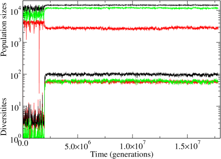
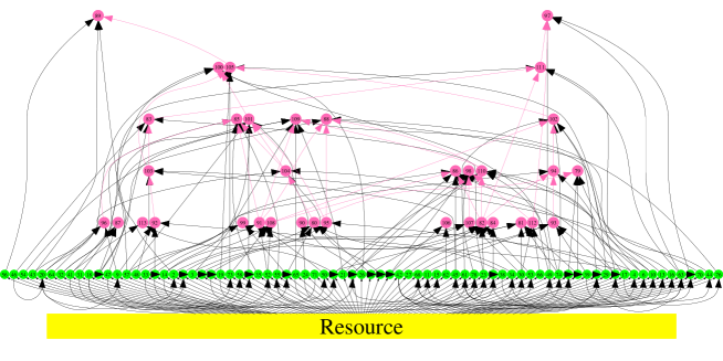
Figure 1: (Top) Time series of populations (upper curves) and diversities (lower curves) for the adaptive model. All species (black), producers (light gray, green online), and consumers (dark gray, red online). (Bottom) A representative food web. The producers are shown just above the external resource. Above them are the consumers, connected to producers by black arrows and to other consumers by gray (pink online) arrows. Arrows point from prey to predator.

As the model is defined above, species forage indiscriminately over all available resources, with the output only limited by competition. Also, there is an implication that an individual’s total foraging effort increases proportionally with the number of species to which it is connected by a positive $M_{IJ}$. A more realistic picture would be that an individual’s total foraging effort is constant and can either be divided equally, or concentrated on richer resources. This is known as adaptive foraging. While one can go to great length devising optimal foraging strategies DROS01B ; DROS04 , we here only use a simple scheme, in which individuals of $I$ show a preference for prey species $J$, based on the interactions and population sizes (uncorrected for interspecies competition) and given by

$$g_{IJ}=\frac{M_{IJ}n_{J}}{\eta_{I}R+\sum_{K}^{{\rm prey}(I)}M_{IK}n_{K}}\;,$$ (5)

and analogously for $R$ by $g_{IR}={\eta_{I}R}/[{\eta_{I}R+\sum_{K}^{{\rm prey}(I)}M_{IK}n_{K}}]$. The total foraging effort is thus $g_{IR}+\sum_{J}^{{\rm prey}(I)}g_{IJ}=1$. These preference factors are used to modify the reproduction probabilities by replacing all occurrences of $M_{IJ}$ by $M_{IJ}g_{IJ}$ and of $\eta_{I}$ by $\eta_{I}g_{IR}$ in Eqs. (1) – (3).

II Numerical Results

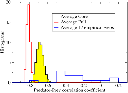
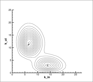
Figure 2: (Left) Correlations between indegree (number of prey) and outdegree (number of predators) for full and core communities and 17 empirical communities RIKV06 . (Right) Joint probability distribution for indegree and outdegree in core communities. The simulation results in both parts were averaged over 327 680 communities.

We simulated the model over $2^{24}=16\,777\,216$ generations (plus $2^{20}$ generations “warm-up”) for the following parameters: $L=21$ ($2^{21}=2\,097\,152$ potential species), $R=16\,000$, $F=2$, $\mu=10^{-3}$, $c_{\rm prod}=0.05$, interaction matrix $\bf M$ with connectance $C=0.1$ and nonzero elements with a symmetric, triangular distribution over $[-1,+1]$, and $\lambda=1.0$. We ran five independent runs, each starting from a population of 100 randomly chosen producer species.

Time series of diversities (effective numbers of species) and population sizes for one run are shown in Fig. 1(top). To filter out noise from low-population, unsuccessful mutants, the diversity is defined as the exponential Shannon-Wiener index KREB89 . This is the exponential function of the information-theoretical entropy of the population distributions, $\rho_{I}(t)=n_{I}(t)/N_{\rm tot}(t)$ for the case of all species, and analogously for the producers and consumers separately.

Without adaptive foraging, the system flips randomly between a phase with a diversity near ten, and a phase of one or a few producer species with a very low population of many unstable consumer species RIKV09 . Adaptive foraging produces a striking change in the dynamics. There is now a metastable low-diversity phase, which gives way at a random time to a stable high-diversity phase with much smaller fluctuations. As seen in Fig. 1(top), the switch-over is quite abrupt.

A representative community food web is shown in Fig. 1(bottom). This is a “core community,” extracted from the full community by retaining only species with $n_{I}>1$ that also existed 256 generations earlier. Here, every consumer species preys on at least one producer species, thus there are only two trophic levels. (Only links with $|M_{IJ}|\geq 0.5$ are included.)

Histograms of the correlation coefficient between a species’ numbers of prey (indegree) and predators (outdegree) are shown in Fig. 2(left). The correlations are strongly negative in both the simulated full and core communities and also in the majority of the 17 empirical communities considered in Ref. RIKV06 . These negative correlations are explained by the joint indegree-outdegree distribution shown in Fig. 2(right): producers (P) have low average indegree and high average outdegree, while consumers (C) show the opposite behavior.

III Conclusions

We have introduced a model for the biological coevolution of predators and prey, based on the ecological concept of functional response. When adaptive foraging is included in the model, it has a dynamically stable phase of relatively high diversity. The indegree and outdegree of a species are negatively correlated, which is explained by the observation that producers have low indegree and high outdegree, while consumers have high indegree and low outdegree. Our model demonstrates the high degree of complexity that can be produced, even by simple models of biological evolution and ecology.

References

- (1) B. Drossel, Adv. Phys. 50 (2001) 209.
- (2) P. A. Rikvold and R. K. P. Zia, Phys. Rev. E 68 (2003) 031913.
- (3) P. A. Rikvold and V. Sevim, Phys. Rev. E 75 (2007) 051920.
- (4) B. Drossel, P. G. Higgs, and A. J. McKane, J. Theor. Biol. 208 (2001) 91.
- (5) C. J. Krebs, Ecology. The Experimental Analysis of Distribution and Abundance. Fifth Edition, Benjamin Cummings, San Francisco, 2001.
- (6) G. T. Skalski and J. F. Gilliam, Ecology 82 (2001) 3083.
- (7) B. Drossel, A. McKane, and C. Quince, J. Theor. Biol. 229 (2004) 539.
- (8) N. D. Martinez, R. J. Williams, and J. A. Dunne, in Ecological Networks: Linking structure to dynamics in food webs, edited by M. Pasqual and J. A. Dunne, Oxford University Press, Oxford, 2006, pp. 163–185.
- (9) H. Resit, R. Arditi, and L. R. Ginzburg, Ecology 76 (1995) 995.
- (10) W. M. Getz, J. Theor. Biol. 108 (1984) 623.
- (11) C. J. Krebs, Ecological Methodology, Harper & Row, New York, 1989, chap. 10.
- (12) P. A. Rikvold, Ecol. Complex., DOI:10/1016/j.ecocom.2009.08.007 (2009).