Zeta-functions of certain $K3$ fibered Calabi–Yau threefolds

Abstract.

We consider certain $K3$-fibered Calabi–Yau threefolds. One class of such Calabi–Yau threefolds are constructed by Hunt and Schimmrigk in [13] using twist maps. They are realized in weighted projective spaces as orbifolds of hypersurfaces. Our main goal of this paper is to investigate arithmetic properties of these $K3$-fibered Calabi–Yau threefolds. In particular, we give detailed discussions on the construction of these Calabi–Yau varieties, singularities and their resolutions. We then determine the zeta-functions of these Calabi–Yau varieties. Next we consider deformations of our $K3$-fibered Calabi–Yau threefolds, and we study the variation of the zeta-functions using $p$-adic rigid cohomology theory.

1. Introduction

We will study the so-called split-type (or product-type) Calabi–Yau threefolds. By this, we mean Calabi–Yau threefolds with fibrations of lower-dimensional Calabi–Yau varieties, that is, with elliptic, or $K3$ fibrations, or both. Hunt and Schimmrigk [13] described a method of constructing such split-type Calabi–Yau threefolds using twist maps, and showed many examples defined by hypersurfaces of diagonal (or Fermat) type in weighted projective spaces. In this paper, we also consider non-diagonal hypersurfaces which we call quasi-diagonal threefolds. They have many geometric properties in common with the diagonal type and they are birational to some quotient of diagonal threefolds. But, their arithmetic is slightly different and allows us to construct many more interesting examples. (For arithmetic purposes, we may work on more general hypersurfaces such as weighted Delsarte hypersurfaces.)

The Calabi–Yau threefolds constructed in this paper, except for those discussed in Sections 10 to 12, have components of diagonal or quasi-diagonal hypersurfaces and they are of CM type in the sense that their Hodge groups are commutative. However, when hypersurfaces used in our construction are not of diagonal type, it is very unlikely that the quotient varieties are to be of CM type. For instance, deformations of our Calabi–Yau threefolds are not of CM type.

In the earlier sections of this paper, we describe how to construct split-type Calabi–Yau threefolds. The way we construct the Calabi–Yau threefolds is as follows: let $S$ be a surface and $C$ be a curve, and take a product $S\times C$. Assume that a finite group $\boldsymbol{\mu}$ acts on both $S$ and $C$. Then define the quotient $V:=S\times C/\boldsymbol{\mu}$ by this action of $\boldsymbol{\mu}$. Resolving its singularities, we obtain a Calabi–Yau threefold $\tilde{V}$. We focus our attention on the case where $\boldsymbol{\mu}$ is a cyclic group acting on one variable of each component. Then $V$ is birational to a quasi-smooth weighted hypersurface $X$ and we can use toroidal desingularizations on $X$ to construct a resolution $\tilde{V}$. In fact, singularities of $X$ are easier to handle than those of $V$ so that we can keep track of the fields of definition under desingularization. This is important for arithmetic investigations.

The construction of $\tilde{V}$ from a product $S\times C$ naturally induces fibrations on $\tilde{V}$. They are dependent on the choice of each component. We consider the cases where $\tilde{V}$ has $K3$ and/or elliptic fibrations, as done in the paper of Hunt and Schimmrigk [13].

We will then determine the zeta-functions of split-type Calabi–Yau threefolds. We discuss the cases where both $S$ and $C$ are defined by either diagonal or quasi-diagonal equations, so that $\tilde{V}$ is birational to a hypersurface of diagonal or quasi-diagonal type in a weighted projective $4$-space. The zeta-functions of such hypersurfaces are computed by using Weil’s method Our task is therefore to determine their singularities and resolutions explicitly to describe the zeta-function of $\tilde{V}$.

In order to express their zeta-functions in a simple form, we compute them over some finite extensions of $\mathbb{F}_{p}$. But, by calculating them over several extensions of $\mathbb{F}_{p}$, we can determine zeta-functions over $\mathbb{F}_{p}$. We explain the idea of this in Section 8 (cf. Lemma 8.2 and Remark 8.3) and discuss more details in a subsequent paper. Also, our zeta-functions in Sections 8 and 9 are described in terms of Jacobi sums. They are endowed with a group action which induces a natural decomposition (called motivic decomposition) of zeta-functions. This is explained, for instance, in [11] and [24] and we investigate more details about this in a subsequent paper.

Now the étale cohomology groups of $\tilde{V}$ are built up from those of components by the Künneth formula. The eigenvalues of the Frobenius map on the étale cohomology groups of $\tilde{V}$ are products of the eigenvalues of the components which are compatible with the finite group actions. We compute the zeta-functions of $K3$-fibered Calabi–Yau threefolds, using the splitting property, and computing eigenvalues of Frobenius for the components which are compatible with group actions.

Next, we will study the variation of the zeta-functions of the Calabi–Yau threefolds considered in the previous sections. Some deformations can be constructed by twist maps, but not in general. We ought to introduce a different cohomology theory to study the zeta-functions, namely the $p$-adic rigid cohomology theory.

The paper is organized as follows.

In Section $2$, we review some facts on weighted diagonal hypersurfaces and twist maps, respectively, which are needed for the subsequent discussions. In Sections $3$ and $4$, we construct $K3$-fibered or elliptic fibered Calabi–Yau threefolds via twist maps. We start with the product $C\times Y$ where $C$ is a curve and $Y$ is a surface. The twist map induces a group action, $\boldsymbol{\mu}$, on the product $C\times Y$ and we take the quotient $V=C\times Y/\boldsymbol{\mu}$. Resolving singularities of $V$, we obtain a Calabi–Yau threefold with $K3$ or elliptic fibration. We list various examples of these using diagonal or quasi-diagonal hypersurfaces in weighted projective spaces.

In Section $5$, we study in detail singularities appearing in our constructions. We choose $C$ and $S$ to be quasi-smooth curves and surfaces, so that they have cyclic quotient singularities. In our case, $V=S\times C/\boldsymbol{\mu}$ is birational to a quasi-smooth hypersurface $X$ which has at most cyclic quotient singularities.

In Section $6$, we consider resolutions of singularities. Since weighted projective spaces are toric varieties, we can employ toric desingularizations and they also resolve singularities of quasi-smooth subvarieties $X$. To find a crepant resolution of $X$ (when it is Calabi–Yau) however, we usually need only a partial desingularization of the ambient space. We describe an algorithm for it and give several examples of explicit resolutions. We also discuss the field of definition for such resolutions and exceptional divisors.

In Section $7$, we compute the cohomology groups of smooth Calabi–Yau threefolds constructed from the products $C\times S$ where $C$ is a diagonal curve and $S$ a diagonal surface. In Sections $8$ and $9$, we explicitly calculate the zeta-functions of our Calabi–Yau threefolds.

From Section $10$ on, we consider a family of quasi-smooth hypersurfaces, focusing on a two-parameter family. Some of the deformations may not be constructed from the twist map. We compute the zeta-function of the family using rigid cohomology theory. In Section $11$, the deformation matrix is computed in terms of hypergeometric functions. In the final section $12$, an explicit example is discussed.

In this paper, our discussions are focused on the local arithmetic, namely, the determination of the zeta-functions of our Calabi–Yau varieties. In subsequent papers, we plan to give global considerations and hope to determine the $L$-series of our Calabi–Yau varieties and discuss their modularity (at least at the motivic level.) Also, in this article, we have not fully utilized elliptic or $K3$-fibrations in our arithmetic quests, and this is left as a topic of our future investigation. This involves some function fields arithmetic of elliptic curves or $K3$ surfaces.

Acknowledgments Y. Goto’s research was partially supported by the Grants-in-Aid for Scientific Research (C) 18540005 and 21540003 of the Japan Society for the Promotion of Science (JSPS). The second author wishes to thank the third author for the invitation to Queen’s University and he wishes to thank Queen’s University for their hospitality. N. Yui was supported in part by a Discovery Grant of Natural Science Research Council of Canada (NSERC). During the preparation of this paper, N. Yui held a visiting professorship at various institutions. This includes Fields Institute (Toronto), Tsuda College (Tokyo) and Nagoya University (Nagoya). She thanks these institutions for their hospitality and support.

2. Preamble: weighted diagonal hypersurfaces

We first recall the definition of weighted projective spaces, which are realized as certain singular quotients of the usual projective spaces. The standard references on weighted projective spaces are Dolgachev [6] and Dimca [4]. Let $k$ be a field and fix an algebraic closure $\overline{k}$ of $k$. For instance, $k=\mathbb{Q}$ or $k=\mathbb{F}_{q}$, a finite field of characteristic $p=char(k)$ with $q$ elements. In this section, we work only over $\overline{k}$ and often omit to specify the field of definition. Let $(w_{0},w_{1},\cdots,w_{n})\in\mathbb{N}^{n+1}$ be a weight. When $k=\mathbb{F}_{q}$, assume that $\mbox{gcd}(q,w_{i})=1$ for every $i$. We may assume without loss of generality that weights are normalized, that is, no $n$ of the $n+1$ weights have common divisor $>1$. For each $i,0\leq i\leq n$, let $\boldsymbol{\mu}_{w_{i}}$ denote the group of $w_{i}$-th roots of unity. Let $\boldsymbol{\mu}:=\boldsymbol{\mu}_{w_{0}}\times\cdots\times\boldsymbol{\mu}_{w_{n}}$ act on the usual projective $n$-space $\mathbb{P}^{n}$ as follows: For $\mathbf{g}=(g_{0},g_{1},\cdots,g_{n})\in\boldsymbol{\mu}$ and for the homogeneous coordinate $\mathbf{z}=(z_{0}:z_{1}:\cdots:z_{n})$ on $\mathbb{P}^{n}$, the action is given by

$$(\mathbf{g},\mathbf{z})\mapsto(g_{0}z_{0}:\cdots:g_{n}z_{n}).$$

The quotient $\mathbb{P}^{n}/\boldsymbol{\mu}$ is a weighted projective $n$-space and denoted by $\mathbb{P}^{n}(w_{0},\mathbf{w})=\mathbb{P}^{n}(w_{0},w_{1},\cdots,w_{n})$ where we put $\mathbf{w}=(w_{1},\cdots,w_{n})$. The usual projective space $\mathbb{P}^{n}$ is identified with $\mathbb{P}^{n}(1,1,\cdots,1)$. A weighted hypersurface $V$ is the zero locus of a weighted homogeneous polynomial. Such $V$ is said to be transversal if the singular locus of $V$ is contained in the singular locus of $\mathbb{P}^{n}(w_{0},\mathbf{w})$, and quasi-smooth if the affine cone of $V$ is smooth outside the vertex.

In this paper, we take the products of quasi-smooth weighted projective hypersurfaces of diagonal type and consider their quotients under the action of finite groups.

Let $d$ be a positive integer such that $w_{i}\mid d$ for every $i$ $(0\leq i\leq n)$ and write $d_{i}:=d/w_{i}$. The weighted hypersurface, $V$, defined by the equation

$$c_{0}x_{0}^{d_{0}}+c_{1}x_{1}^{d_{1}}+\cdots+c_{n}x_{n}^{d_{n}}=0\qquad(c_{i}\neq 0)$$

will be called a weighted diagonal hypersurface of degree $d$ in $\mathbb{P}^{n}(w_{0},w_{1},\cdots,w_{n})$. $V$ is quasi-smooth if and only if $d_{i}\neq 0$ in $k$ for $0\leq i\leq n$. For simplicity, we consider the case where the coefficients are $c_{0}=c_{1}=\cdots=c_{n}=1$, namely the hypersurface

$$x_{0}^{d_{0}}+x_{1}^{d_{1}}+\cdots+x_{n}^{d_{n}}=0$$

(it may be called the weighted Fermat hypersurface of degree $d$).

We note that weighted diagonal hypersurfaces of degree $d$ enjoy the same geometry as weighted Fermat hypersurfaces of degree $d$. However, their arithmetic properties are different. For instance, when $V$ is a surface over $\mathbb{F}_{q}$ or $\mathbb{Q}$, bringing in non-trivial coefficients $c_{i}$ allows us to construct examples of surfaces with particularly small (or large) Picard numbers over $\mathbb{F}_{q}$ or $\mathbb{Q}$.

Write $Q:=(w_{0},w_{1},\cdots,w_{n})$ and let $V$ be the weighted diagonal hypersurface of degree $d$ in $\mathbb{P}^{n}(Q)$. $V$ is of dimension $n-1$ and its properties are investigated by various authors (see, for instance, [8] and [23]). Here we recall its cohomology groups. Choose a prime $\ell$ different from $\mbox{char}\,(k)$. Let $H^{i}(V,\mathbb{Q}_{\ell})$ denote the $i$-th $\ell$-adic étale cohomology group of $V$ over $\overline{k}$. If $i\neq\dim V=n-1$, we have

$$H^{i}(V,\mathbb{Q}_{\ell})\cong\begin{cases}\mathbb{Q}_{\ell}&\mbox{ if $i$ is even }\\ \{0\}&\mbox{ if $i$ is odd }\end{cases}$$

and for $i=n-1$, $H^{n-1}(V,\mathbb{Q}_{\ell})$ is decomposed into a direct sum of one-dimensional subspaces as follows: let $H^{n-1}_{prim}(V,\mathbb{Q}_{\ell})$ denote the primitive part of the cohomology $H^{n-1}(V,\mathbb{Q}_{\ell})$, namely

$$H^{n-1}(V,\mathbb{Q}_{\ell})\cong\begin{cases}H^{n-1}_{prim}(V,\mathbb{Q}_{\ell})&\mbox{ if $\dim V$ is odd }\\ V(0)\oplus H^{n-1}_{prim}(V,\mathbb{Q}_{\ell})&\mbox{ if $\dim V$ is even }\end{cases}$$

where $V(0)$ denotes the subspace corresponding to the hyperplane section. Let

$$\mathfrak{A}_{n-1}(Q):=\biggl{\{}\mathbf{a}=(a_{0},a_{1},\cdots,a_{n})\,|\,a_{i}\in(w_{i}\mathbb{Z}/d\mathbb{Z}),a_{i}\neq 0,\sum_{i=0}^{n}a_{i}\equiv 0\pmod{d}\biggr{\}}.$$

Then for $V$ over $\overline{k}$, we have a decomposition

(2.1) $$H^{n-1}_{prim}(V,\mathbb{Q}_{\ell})\cong\bigoplus_{\mathbf{a}\in\mathfrak{A}_{n-1}}V(\mathbf{a})$$

where

$$V(\mathbf{a})=\{v\in H^{n-1}_{prim}(V,\mathbb{Q}_{\ell})\mid\gamma^{*}(v)={\zeta}_{0}^{a_{0}}{\zeta}_{1}^{a_{1}}\cdots{\zeta}_{n}^{a_{n}}v,\ \forall\gamma=({\zeta}_{0},{\zeta}_{1},\cdots,{\zeta}_{n})\in\Gamma\}$$

with

$$\Gamma:=\mu_{d_{0}}\times\mu_{d_{1}}\times\cdots\times\mu_{d_{n}}/(\mbox{diagonal elements}),$$

$\mu_{d}$ is the group of $d$-th roots of unity in $\overline{k}$ and $\gamma^{*}$ is the automorphism of $H^{n-1}_{prim}(V,\mathbb{Q}_{\ell})$ induced by $\gamma$. (Here we choose a prime $\ell$ satisfying $\ell\equiv 1\pmod{d}$ so that $\mu_{d}$ can be embedded into $\mathbb{Q}_{\ell}$ multiplicatively.)

For the product of two weighted diagonal hypersurfaces, we have the Künneth formula to compute its cohomology and we find

(2.2) $$H^{j}(V_{1}\times V_{2},\mathbb{Q}_{\ell})=\bigoplus_{i_{1}+i_{2}=j}H^{i_{1}}(V_{1},\mathbb{Q}_{\ell})\otimes H^{i_{2}}(V_{2},\mathbb{Q}_{\ell}).$$

Since $H^{i_{1}}(V_{1},\mathbb{Q}_{\ell})$ and $H^{i_{2}}(V_{2},\mathbb{Q}_{\ell})$ are decomposed into one-dimensional pieces, so is $H^{j}(V_{1}\times V_{2},\mathbb{Q}_{\ell})$ and each summand takes such a form as $V(\mathbf{a})\otimes V(\mathbf{b})$. In later sections, we look at the case where $V_{1}$ is a curve and $V_{2}$ is a surface so that $V_{1}\times V_{2}$ is a threefold.

Let $V_{1}$ and $V_{2}$ be weighted diagonal hypersurfaces and write $Y:=V_{1}\times V_{2}$. The direct product $\Gamma_{V_{1}}\times\Gamma_{V_{2}}$ acts on $Y$ component-wise. In this paper, we choose a subgroup, $\Gamma_{Y}$, of $\Gamma_{V_{1}}\times\Gamma_{V_{2}}$ and consider the quotient variety

$$X:=Y/\Gamma_{Y}.$$

Since $\Gamma_{Y}$ is a finite abelian group, $X$ has at most abelian quotient singularities.

The quotient variety $X=Y/\Gamma_{Y}$ is usually singular. But if the order of $\Gamma_{Y}$ is invertible in $k$, we can compute the cohomology of $X$ as the $\Gamma_{Y}$-invariant subspace of the cohomology of $Y$. For this, we work over an algebraic closure $\overline{k}$ of $k$. Write $p:=\mbox{char}\,(k)$ and assume $(p,\#\Gamma_{Y})=1$. We choose a prime $\ell$ satisfying $\ell\equiv 1\pmod{d}$. It is known that the $\ell$-adic étale cohomology satisfies

(2.3) $$H^{i}(X,\mathbb{Q}_{\ell})\cong H^{i}(Y,\mathbb{Q}_{\ell})^{\Gamma_{Y}}$$

for every $i$ $(0\leq i\leq 2\dim Y)$. (In fact, the Hochschild-Serre spectral sequence holds for $Y$ and the Galois cohomology for a finite group $\Gamma_{Y}$ vanishes by tensoring with $\mathbb{Q}_{\ell}$. This yields the isomorphism in question.)

3. Twist maps

In this section, we recall the method of Hunt and Schimmrigk [13] to construct $K3$ fibered Calabi–Yau threefolds as quotients of weighted hypersurfaces not necessarily of diagonal type, using the twist maps. This construction is a generalization of the construction Shioda and Katsura [21] for non-singular hypersurfaces in the usual projective spaces. We will describe the construction of quotients of weighted hypersurfaces by twist maps in any dimension.

Let $V_{1}$ and $V_{2}$ be two weighted hypersurfaces defined as follows.

$$\begin{split}V_{1}:=&\{x_{0}^{\ell}+f(x_{1},\cdots,x_{n})=0\}\subset\mathbb{P}^{n}(w_{0},\mathbf{w})\quad\mbox{deg}(V_{1})=\ell w_{0}\\ V_{2}:=&\{y_{0}^{\ell}+g(y_{1},\cdots,y_{m})=0\}\subset\mathbb{P}^{m}(v_{0},\mathbf{v})\quad\mbox{deg}(V_{2})=\ell v_{0}\end{split}$$

where $\mathbf{w}=(w_{1},\cdots,w_{n})$ and $\mathbf{v}=(v_{1},\cdots,v_{m})$ and both $f$ and $g$ are assumed to be quasi-smooth, and so are $V_{1}$ and $V_{2}$. Consider the hypersurface:

$$X:=\{f(z_{1},\cdots,z_{n})-g(t_{1},\cdots,t_{m})=0\}\subset\mathbb{P}^{n+m-1}(v_{0}\mathbf{w},\,w_{0}\mathbf{v}).$$

where ${\mbox{deg}}(X)=v_{0}w_{0}\ell=v_{0}{\mbox{deg}}(f)=w_{0}{\mbox{deg}}(g)$.

In order to define the twist map we need to assume that $\gcd(v_{0},w_{0})=1$. This condition seems to be missing in [13]. If this is the case then fix $s_{0},t_{0}\in\mathbb{Z}$ such that $0\leq s_{0}<v_{0}$, $0\leq t_{0}<w_{0}$, $s_{0}w_{0}+1\equiv 0\bmod v_{0}$ and $t_{0}v_{0}+1\equiv 0\bmod w_{0}$. Let $s=(s_{0}w_{0}+1)/v_{0}$ and $t=(t_{0}v_{0}+1)/w_{0}$. Note that $s,t$ are non-zero integers.

Definition 3.1.

The rational map

$$\Phi:\mathbb{P}^{n}(w_{0},\mathbf{w})\times\mathbb{P}^{m}(v_{0},\mathbf{v})\dashrightarrow\mathbb{P}^{n+m-1}(v_{0}\mathbf{w},w_{0}\mathbf{v})$$

$$\begin{split}((x_{0},x_{1},\cdots,x_{n}),\quad&(y_{0},y_{1},\cdots,y_{m}))\mapsto\\ &(x_{0}^{s_{0}w_{1}}y_{0}^{tw_{1}}x_{1},\cdots,x_{0}^{s_{0}w_{n}}y_{0}^{tw_{n}}x_{n},\,x_{0}^{sv_{1}}y_{0}^{t_{0}v_{1}}y_{1},\cdots,x_{0}^{sv_{m}}y_{0}^{t_{0}v_{m}}y_{m})\end{split}$$

restricted to $V_{1}\times V_{2}$ is a generically rational finite map onto $X$. The map $\Phi$ is called the twist map.

Remark 3.1.

In [13] a slightly different definition of the twist map is given, namely

$$\begin{split}((x_{0},x_{1},\cdots,x_{n}),\quad&(y_{0},y_{1},\cdots,y_{m}))\mapsto\\ &(y_{0}^{w_{1}/w_{0}}x_{1},\cdots,y_{0}^{w_{n}/w_{0}}x_{n},\,x_{0}^{v_{1}/v_{0}}y_{1},\cdots,x_{0}^{v_{m}/v_{0}}y_{m}).\end{split}$$

If $v_{0}$ or $w_{0}$ is different from 1 then one takes some $v_{0}$-th or $w_{0}$-th roots of $x_{0}$ or $y_{0}$. It is not directly clear that this map is a rational map, that is, can be given in terms of polynomials. In [13] it is then argued that this map is well-defined, but no proof is given for the fact that this map is given by polynomials. Below, we construct a counterexample to the claim of Hunt and Schimmrigk where the twist map is neither a polynomial map nor well-defined.

Remark 3.2.

The rational map $\Phi$ can be extend to points with $x_{0}=0$ and $y_{0}\neq 0$ as follows

$$\begin{split}((0,x_{1},\cdots,x_{n}),\quad&(y_{0},y_{1},\cdots,y_{m}))\mapsto\\ &(x_{1},\cdots,x_{n},\,0,\cdots,0)\end{split}$$

A similar extension exists for points with $x_{0}\neq 0$ and $y_{0}=0$. The map $\Phi$ is not defined at points with $x_{0}=y_{0}=0$.

Remark 3.3.

The condition $\gcd(v_{0},w_{0})=1$ is necessary, both for our definition and for the definition in [13]. We give an example for which the twist map, as defined in [13], is not well-defined.

Take $\mathbf{w}=\mathbf{v}=(2,1,1)$. Let $V_{1}=\{x_{0}^{2}+x_{1}^{4}+x_{2}^{4}\}$ and $V_{2}=\{y_{0}^{2}+y_{1}^{4}+y_{2}^{4}\}$. The twist map of [13] in this case should be the rational map $\mathbb{P}^{2}(2,1,1)\times\mathbb{P}^{2}(2,1,1)\rightarrow\mathbb{P}^{3}(2,2,2,2)=\mathbb{P}^{3}$ given by

$$(x_{0},x_{1},x_{2})\times(y_{0},y_{1},y_{2})\mapsto(\sqrt{y_{0}}x_{1},\sqrt{y_{0}}x_{2},\sqrt{x_{0}}y_{1},\sqrt{x_{0}}y_{2}).$$

This map is not well-defined, since it depends on the choice of $\sqrt{x_{0}y_{0}}$.

Now we let the group $\boldsymbol{\mu}_{\ell}$ of $\ell$-th roots of unity act on $V_{1}\times V_{2}\subset\mathbb{P}^{n}(w_{0},\mathbf{w})\times\mathbb{P}^{m}(v_{0},\mathbf{v})$ by $\gamma\in\boldsymbol{\mu}_{\ell}$. The action is defined as follows.

Definition 3.2.

Assume that $\gcd(w_{0},v_{0},\ell)=1$. Then the group $\boldsymbol{\mu}_{\ell}$ acts on $V_{1}\times V_{2}$ by

$$(\gamma,(x_{0}:\cdots:x_{n}),\,(y_{0}:\cdots:y_{m}))\mapsto((\gamma x_{0}:x_{1},\cdots:x_{n}),(\gamma y_{0}:y_{1},\cdots:y_{m})).$$

for every $\gamma\in\boldsymbol{\mu}_{\ell}$.

The quotient space $V_{1}\times V_{2}/{\boldsymbol{\mu}_{\ell}}$ is a projective variety and the rational map $V_{1}\times V_{2}\to X$ is generically $\ell:1$.

$$\begin{array}[]{ccc}V_{1}\times V_{2}&\small{\Phi\mid_{V_{1}\times V_{2}}}&\\ \downarrow&\searrow&\\ V_{1}\times V_{2}/{\boldsymbol{\mu}_{\ell}}&\cdots\rightarrow&X\end{array}$$

Now we discuss singularities on the varieties $V_{1}\times V_{2}/{\boldsymbol{\mu}_{\ell}}$ and $X$. First we know that only singularities occurring in ambient weighted projective spaces are cyclic quotient singularities. Since $f$ and $g$ are quasi-smooth, so are $V_{1}$ and $V_{2}$, and they have cyclic quotient singularities all due to the ambient spaces. Further, a threefold $X$ is defined by $f-g$ and $f$ and $g$ have no common variable. Hence $X$ is also quasi-smooth and it possesses at most cyclic quotient singularities.

Cyclic quotient singularities are resolved by toroidal resolutions and moreover quasi-smooth varieties can be desingularized by applying toroidal resolutions to their ambient spaces. An example is that we obtain a resolution of $X$ by restricting a resolution of $\mathbb{P}^{n+m-1}(v_{0}\mathbf{w},\,w_{0}\mathbf{v})$ onto $X$. We note that it is often sufficient to take a partial resolution of $\mathbb{P}^{n+m-1}(v_{0}\mathbf{w},\,w_{0}\mathbf{v})$ to desingularize $X$; we explain this in Section 6.

On the other hand, $V_{1}\times V_{2}$ and $V_{1}\times V_{2}/{\boldsymbol{\mu}_{\ell}}$ are no longer quasi-smooth in most cases and they have abelian quotient singularities. As $V_{1}\times V_{2}/{\boldsymbol{\mu}_{\ell}}$ is birational to $X$, we may work on $X$ (rather than on $V_{1}\times V_{2}/{\boldsymbol{\mu}_{\ell}}$) to construct their smooth models and discuss their Calabi–Yau properties.

Let $\pi_{X}:\tilde{X}\to X$ be a smooth resolution of $X$. A natural question is When is $\tilde{X}$ Calabi–Yau?

In search of an answer to this question, we will look into the fibrations. Project the quotient $V_{1}\times V_{2}/\boldsymbol{\mu}_{\ell}$ (via $V_{1}/\mu_{\ell}\times V_{2}/\mu_{\ell}$) to the first and the second components, respectively. This gives rise to the following two rational fibrations:

$$\phi_{1}:\tilde{X}\to V_{1}/\boldsymbol{\mu}_{\ell}\quad\mbox{and}\quad\phi_{2}:\tilde{X}\to V_{2}/\boldsymbol{\mu}_{\ell}.$$

$$\begin{matrix}\quad&X&\quad\\ \phi_{1}\swarrow&\quad&\searrow\phi_{2}\\ \quad&\qquad&\qquad\\ V_{1}/{\mu_{\ell}}\quad\quad&\quad\quad\qquad&V_{2}/{\mu_{\ell}}\end{matrix}$$

If $\pi_{X}:\tilde{X}\to X$ is a smooth resolution, then the composite map $\phi_{1}\circ\pi_{X}$ is a fibration of $\tilde{X}$ onto $V_{1}/\mu_{\ell}$ whose generic fibers are copies of resolutions of $V_{2}$. A similar property holds for the fibration $\phi_{2}$. The situation is illustrated as follows, where $Y_{i}$ denotes a smooth resolution of $V_{i}/\mu_{\ell}$:

$$\begin{matrix}X&\overset{\pi_{X}}{\longleftarrow}&\tilde{X}\\ \phi_{i}\downarrow&\quad\quad&\\ V_{i}/\mu_{\ell}&\overset{\pi_{i}}{\longleftarrow}&Y_{i}\end{matrix}$$

Proposition 3.1.

Suppose that $\tilde{X}$ is Calabi–Yau and $w_{0}>1$. Write $\tilde{\phi_{1}}:=\phi_{1}\circ\pi_{X}$ and let $\tilde{V}_{2}$ be the generic smooth fiber of $\tilde{\phi_{1}}$. Then the rational fibration $\tilde{\phi_{1}}:\tilde{X}\to V_{1}/\mu_{\ell}$ lifts to a genuine fibration $\tilde{X}\to Y_{1}$ for some smooth resolution $Y_{1}$ of $V_{1}/\mu_{\ell}$, if and only if $\tilde{V}_{2}$ is also Calabi–Yau. A similar property holds for $\phi_{2}$.

Proof.

(Cf. Lemma 3.4 in [13].) ∎

The upshot of Proposition 3.1 is that it provides a method of constructing split-type (product-type) Calabi–Yau varieties. That is, a covering of a product is Calabi–Yau if and only if one of the components is Calabi–Yau.

Proposition 3.2.

Let $V_{1}$, $V_{2}$ and $X$ be quasi-smooth varieties as before. Then the following assertions hold.

(1) A sufficient condition for $\tilde{V}_{2}$ to be Calabi–Yau hypersurface is:

$$v_{0}+v_{1}+\cdots+v_{m}=\ell v_{0}=\deg(V_{2}),$$

(2) A sufficient condition for $\tilde{X}$ to be Calabi–Yau hypersurface is:

$$\ell w_{0}v_{0}=w_{0}\sum_{i=1}^{m}v_{i}+v_{0}\sum_{j=1}^{n}w_{j}.$$

Proof.

(Cf. [6]) The Calabi–Yau (sufficient) condition for a hypersurface in weighted projective spaces is that the sum of all weights equal the degree of the variety. ∎

4. Construction of $K3$-fibered Calabi–Yau threefolds via twist maps

Now we apply the construction by twist maps to elliptic curves, $K3$ surfaces, and Calabi–Yau threefolds.

Dimension $1$ Calabi–Yau varieties (Elliptic curves): There are three elliptic curves in weighted projective spaces, that are of diagonal form. They are given as in Table 1. All three elliptic curves have complex multiplication, the first and the third by $\mathbb{Z}[\sqrt{-3}]$ and the second by $\mathbb{Z}[\sqrt{-1}]$.

Table 1. Elliptic curves in weighted projective 2-spaces

$$\begin{array}[]{c|c|c}\hline\cr\hline\cr\#&E_{i}&\mbox{equation}\\ \hline\cr 1&E_{1}&y_{0}^{3}+y_{1}^{3}+y_{2}^{3}=0\subset\mathbb{P}^{2}(1,1,1)\\ \hline\cr 2&E_{2}&y_{0}^{4}+y_{1}^{4}+y_{2}^{2}=0\subset\mathbb{P}^{2}(1,1,2)\\ \hline\cr 3&E_{3}&y_{0}^{6}+y_{1}^{3}+y_{2}^{2}=0\subset\mathbb{P}^{2}(1,2,3)\\ \hline\cr\hline\cr\end{array}$$

Dimension $2$ Calabi–Yau varieties ($K3$ surfaces): Let $C_{(w_{0},w_{1},w_{2})}\in\mathbb{P}^{2}(w_{0},w_{1},w_{2})$ be a curve defined by

$$C_{(w_{0},w_{1},w_{2})}:=\{x_{0}^{\ell}+f(x_{1},x_{2})=0\}\subset\mathbb{P}^{2}(w_{0},w_{1},w_{2})\quad\mbox{with deg $C=\ell w_{0}$}$$

and the group $\mathbb{Z}/\ell\mathbb{Z}$ acts on $C$. Then applying the twist map to $C\times E_{i}$ where $i=1$ (resp. $3$) if $\ell=3$ (resp. $6$), and $i=2$ if $\ell=4$. Each $E_{i}$ has the automorphism group $\mathbb{Z}/\ell\mathbb{Z}$. We take the quotient of the product $C\times E_{i}$ under the action of the group $\mathbb{Z}/\ell\mathbb{Z}$. Then we get a hypersurface $X\subset\mathbb{P}^{3}(v_{0}w_{1},v_{0}w_{2},w_{0}v_{1},w_{0}v_{2})$ of degree $d$, where $(v_{0},v_{1},v_{2})\in\{(1,1,1),(1,1,2),(1,2,3)\}$.

Proposition 4.1.

There are eleven $K3$ surfaces arising from this construction. See Table 2 for the list, where we put $(k_{0},k_{1},k_{2},k_{3})=(v_{0}w_{1},v_{0}w_{2},w_{0}v_{1},w_{0}v_{2})$, $d=\sum_{i=0}^{3}k_{i}$. For $f(x_{1},x_{2})$ and $g(y_{1},y_{2})$, we may take, for instance,

$$f(x_{1},x_{2})=x_{1}^{\ell w_{0}/w_{1}}+x_{2}^{\ell w_{0}/w_{2}}\quad\mbox{and}\quad g(y_{1},y_{2})=-(y_{1}^{\ell v_{0}/v_{1}}+y_{2}^{\ell v_{0}/v_{2}}).$$

In this case, $C_{(w_{0},w_{1},w_{2})}$ is covered by the diagonal curve of degree $d$ in $\mathbb{P}^{2}(1,1,1)$.

Table 2. $K3$ surfaces appearing in our construction

$$\begin{array}[]{c|c|c|c|c|c|c}\hline\cr\hline\cr\#&C_{(w_{0},w_{1},w_{2})}&g(C)&E_{i}&\ell&(k_{0},k_{1},k_{2},k_{3})&d\\ \hline\cr 1&(2,1,1)&4&E_{1}&3&(1,1,2,2)&6\\ \hline\cr 2&&&E_{2}&4&(1,1,2,4)&8\\ \hline\cr 3&&&E_{3}&6&(1,1,4,6)&12\\ \hline\cr 4&(3,1,2)&7&E_{2}&4&(1,2,3,6)&12\\ \hline\cr 5&&&E_{3}&6&(1,2,6,9)&18\\ \hline\cr 6&(4,1,3)&3&E_{1}&3&(1,3,4,4)&12\\ \hline\cr 7&&&E_{3}&6&(1,3,8,12)&24\\ \hline\cr 8&(5,1,4)&6&E_{2}&4&(1,4,5,10)&20\\ \hline\cr 9&(7,1,6)&15&E_{3}&6&(1,6,14,21)&42\\ \hline\cr 10&(5,2,3)&11&E_{3}&6&(2,3,10,15)&30\\ \hline\cr 11&(11,5,6)&5&E_{3}&6&(5,6,22,33)&66\\ \hline\cr\hline\cr\end{array}$$

Remark 4.1.

All $K3$ surfaces can be realized as orbifolds of diagonal or quasi-diagonal hypersurfaces. For instance, $\#3$ may be realized by a diagonal hypersurface $z_{1}^{12}+z_{2}^{12}+z_{3}^{3}+z_{4}^{2}=0\subset\mathbb{P}^{2}(1,1,4,6)$. Similarly $\#8$ may be realized by a diagonal hypersurface $z_{1}^{20}+z_{2}^{5}+z_{3}^{4}+z_{4}^{2}=0\subset\mathbb{P}^{3}(1,4,5,10)$. (By Goto [8], Yonemura [22], there are in total $14$ weighted diagonal K3 surfaces obtained as quotients of diagonal hypersurfaces by finite abelian group actions.) The last example $\#11$ can be realized by the polynomial

$$z_{0}^{12}z_{1}+z_{1}^{11}+z_{2}^{3}+z_{3}^{2}=0\subset\mathbb{P}^{3}(5,6,22,33).$$

Goto [9] considered $K3$ surfaces of the latter kind, the so-called quasi-diagonal $K3$ surfaces.

Dimension $3$ Calabi–Yau varieties (Calabi–Yau threefolds): We now apply the twist map to construct $K3$-fibered Calabi–Yau threefolds, which are the quotients of either $S\times E$, where $S$ is a surface and $E$ is an elliptic curve, or $C\times Y$ where $C$ is a curve and $Y$ is a $K3$ surface in weighted projective spaces, under the action of the group $\mathbb{Z}/\ell\mathbb{Z}$.

(A) Elliptic fibered Calabi–Yau threefolds $S\times E$: Let $(w_{0},\mathbf{w})=(w_{0},w_{1},w_{2},w_{3})$ be a weight, and consider the surface

(4.1) $$S_{(w_{0},w_{1},w_{2},w_{3})}:=\{x_{0}^{\ell}+f(x_{1},x_{2},x_{3})=0\}\subset\mathbb{P}^{3}(w_{0},w_{1},w_{2},w_{3})$$

of degree $\ell w_{0}$.

Apply the twist map to the product $S_{(w_{0},w_{1},w_{2},w_{3})}\times E_{i}$ where $i=1$ (resp. $3$) if $\ell=3$ (resp. $6$), and $i=2$ if $\ell=4$ onto a threefold of degree $=\ell w_{0}$, and for the sake of simplicity, we may take $g(y_{1},y_{2})=-(y_{1}^{\ell v_{0}/v_{1}}+y_{2}^{\ell v_{0}/v_{2}})$.

A natural question is : What combination of weights $(w_{0},w_{1},w_{2},w_{3})$ and $(v_{0},v_{1},v_{2})$ would give rise to Calabi–Yau threefolds?

We divide our constructions into two cases:

$1^{\circ}$: $S_{(w_{0},w_{1},w_{2},w_{3})}$ is not a $K3$ surface.

$2^{\circ}$: $S_{(w_{0},w_{1},w_{2},w_{3})}$ is a $K3$ surface.

Proposition 4.2.

Let $E_{i},\,i\in\{1,2,3\}$ be elliptic curves in Table 1. Suppose that $S_{(w_{0},w_{1},w_{2},w_{3})}$ is not a $K3$ surface. Then there are $14$ elliptically but not $K3$-fibered Calabi–Yau threefolds obtained as quotients of $S_{(w_{0},w_{1},w_{2},w_{3})}\times E_{i}$. Here we put $(k_{0},k_{1},k_{2},k_{3},k_{4})=(v_{0}w_{1},v_{0}w_{2},v_{0}w_{3},w_{0}v_{1},w_{0}v_{2})$ and $d=\sum_{i=0}^{4}k_{i}$. We may take, for instance,

$$f(x_{1},x_{2},x_{3})=x_{1}^{\ell w_{0}/w_{1}}+x_{2}^{\ell w_{1}/w_{0}}+x_{3}^{\ell w_{0}/w_{3}}.$$

With this choice, $S_{(w_{0},w_{1},w_{2},w_{3})}$ is a weighted diagonal surface, though not $K3$.

Table 3. Elliptic but not $K3$-fibered Calabi-Yau threefolds

$$\begin{array}[]{c|c|c|c|c|c|c|c|c}\hline\cr\hline\cr\#&(w_{0},w_{1},w_{2},w_{3})&E_{i}&\ell&(k_{0},k_{1},k_{2},k_{3},k_{4})&d&h^{1,1}&h^{2,1}&\chi\\ \hline\cr 1&(5,1,1,3)&E_{1}&3&(1,1,3,5,5)&15&7&103&-192\\ 2&&E_{3}&6&(1,1,3,10,15)&30&5&251&-492\\ \hline\cr 3&(5,1,1,2)&E_{2}&4&(1,2,2,5,10)&20&6&242&-228\\ 4&&E_{3}&6&(1,2,2,10,15)&30&4&208&-408\\ \hline\cr 5&(7,1,2,4)&E_{2}&4&(1,2,4,7,14)&28&8&116&-216\\ \hline\cr 6&(7,1,3,3)&E_{1}&3&(1,3,3,7,7)&21&17&65&-96\\ 7&&E_{3}&6&(1,3,3,14,21)&42&6&180&-348\\ \hline\cr 8&(7,2,2,3)&E_{3}&6&(2,2,3,14,21)&42&7&151&-288\\ \hline\cr 9&(9,1,4,4)&E_{2}&4&(1,4,4,9,18)&36&19&91&-144\\ \hline\cr 10&(10,2,3,5)&E_{1}&3&(2,3,5,10,10)&30&12&48&-108\\ 11&&E_{3}&6&(2,3,5,20,30)&60&10&106&-192\\ \hline\cr 12&(10,1,3,6)&E_{1}&3&(1,3,6,10,10)&30&19&67&-96\\ 13&&E_{3}&6&(1,3,6,20,30)&60&10&178&-336\\ \hline\cr 14&(13,1,6,6)&E_{3}&6&(1,6,6,26,39)&78&23&143&-240\\ \hline\cr\hline\cr\end{array}$$

The next proposition gives examples of elliptically and $K3$-fibered Calabi–Yau threefolds, which generalize the construction of Livné–Yui [18].

Proposition 4.3.

Let $E_{i}\,(i\in\{1,2,3\})$ be elliptic curves in Table 1, and let $S_{(w_{0},w_{1},w_{2},w_{3})}$ be a $K3$ surface. Then there are $23$ elliptically fibered Calabi–Yau threefolds obtained as quotients of $S_{(w_{0},w_{1},w_{2},w_{3})}\times E_{i}$ where $i\in\{1,2,3\}$, which have also $K3$-fibrations are tabulated in Table 4. Here we put again $(k_{0},k_{1},k_{2},k_{3},k_{4})=(v_{0}w_{1},v_{0}w_{2},v_{0}w_{3},w_{0}v_{1},w_{0}v_{2})$ and $d=\sum_{i=0}^{4}k_{i}$.

For the polynomials $f(x_{1},x_{2},x_{3})$ and $g(y_{1},y_{2})$, we may take

$$f(x_{1},x_{2},x_{3})=x_{1}^{\ell w_{0}/w_{1}}+x_{2}^{\ell w_{0}/w_{2}}+x_{3}^{\ell w_{0}/w_{3}},\qquad g(y_{1},y_{2})=-(y_{1}^{\ell v_{0}/v_{1}}+y_{2}^{\ell v_{0}/v_{2}}).$$

In this case, $S_{(w_{0},w_{1},w_{2},w_{3})}$ is covered by the diagonal surface of degree $d$ in $\mathbb{P}^{3}(1,1,1,1)$.

Table 4. Elliptically and $K3$ fibered Calabi–Yau threefolds

$$\begin{array}[]{c|c|c|c|c|c|c|c}\hline\cr\hline\cr\#&(w_{0},w_{1},w_{2},w_{3})&E_{i}&\ell&(k_{0},k_{1},k_{2},k_{3},k_{4})&d&\chi&K3-\mbox{fiber}\\ \hline\cr 1&(3,1,1,1)&E_{1}&3&(1,1,1,3,3)&9&-216&(1,1,1,3)\\ 2&&E_{2}&4&(1,1,1,3,6)&12&-324&\\ 3&&E_{3}&6&(1,1,1,6,9)&18&-540&\\ \hline\cr 4&(4,1,1,2)&E_{1}&3&(1,1,2,4,4)&12&-192&(1,1,2,4)\\ 5&&E_{2}&4&(1,1,2,4,8)&16&-288&\\ 6&&E_{3}&6&(1,1,2,8,12)&24&-480&\\ \hline\cr 7&(6,1,1,4)&E_{2}&4&(1,1,4,6,12)&24&-312&(1,1,4,6)\\ 8&&E_{3}&6&(1,1,4,12,18)&36&-528&\\ \hline\cr 9&(6,1,2,3)&E_{1}&3&(1,2,3,6,6)&18&-144&(1,2,3,6)\\ 10&&E_{2}&4&(1,2,3,6,12)&24&-480&\\ 11&&E_{3}&6&(1,2,3,12,18)&36&-360&\\ \hline\cr 12&(8,1,1,6)&E_{1}&3&(1,1,6,8,8)&24&-240&(1,3,4,4)\\ 13&&E_{3}&6&(1,1,6,16,24)&48&-624&\\ \hline\cr 14&(8,1,3,4)&E_{3}&6&(1,3,4,16,24)&48&-312&(1,1,4,6)\\ \hline\cr 15&(8,2,3,3)&E_{3}&6&(2,3,3,16,24)&48&-240&(1,3,8,12)\\ \hline\cr 16&(9,1,2,6)&E_{2}&4&(1,2,6,9,18)&36&-228&(1,2,6,9)\\ 17&&E_{3}&6&(1,2,6,18,27)&54&-408&\\ \hline\cr 18&(9,2,3,4)&E_{2}&4&(2,3,4,9,18)&36&-120&(1,2,3,6)\\ \hline\cr 19&(10,1,1,8)&E_{2}&4&(1,1,8,10,20)&40&-432&(1,4,5,10)\\ \hline\cr 20&(10,3,3,4)&E_{3}&6&(3,3,4,20,30)&60&-192&(2,3,10,15)\\ \hline\cr 21&(12,1,2,9)&E_{1}&3&(1,2,9,12,12)&36&-168&(1,3,4,4)\\ 22&&E_{3}&6&(1,2,9,24,36)&72&-240&\\ \hline\cr 23&(14,1,1,12)&E_{3}&6&(1,1,12,28,42)&84&-960&(1,6,14,21)\\ \hline\cr\hline\cr\end{array}$$

Remark 4.2.

With our choice of the polynomials $f(x_{1},x_{2},x_{3})$ and $g(y_{1},y_{2})$, all Calabi–Yau threefolds constructed in Propositions 5.2 and 5.3 can also be realized as orbifolds of diagonal hypersurfaces defined by the equation:

$$V:x_{0}^{d}+x_{1}^{d}+x_{2}^{d}+x_{3}^{d}+x_{4}^{d}=0\subset\mathbb{P}^{4}$$

of degree $d$. Take a finite abelian group $\boldsymbol{\mu}=\boldsymbol{\mu}_{k_{0}}\times\cdots\times\boldsymbol{\mu}_{k_{4}}$, where $\boldsymbol{\mu}_{k_{i}}=\mbox{Spec}(\mathbb{Q}[T]/(T^{k_{i}}-1)$. Now we impose the condition that each $k_{i}$ divides $d$. Then $\boldsymbol{\mu}$ acts on $V$ component-wise. Then a smooth resolution of the quotient $V/\boldsymbol{\mu}$ is a Calabi–Yau threefold in the weighted projective space $\mathbb{P}^{4}(k_{0},k_{1},k_{2},k_{3},k_{4})$ only when $d=k_{0}+k_{1}+\cdots+k_{4}$. This construction was carried out in Yui [23].

With different choices of homogeneous polynomials $f(x_{1},x_{2},x_{3})$ and $g(y_{1},y_{2})$, we may obtain more defining equations for these Calabi–Yau hypersurfaces.

Next we list Calabi–Yau threefolds with elliptic fibrations that are not realized as orbifolds of diagonal hypersurfaces.

Proposition 4.4.

Take the product $S_{(w_{0},w_{1},w_{2},w_{3})}\times E_{3}$, where $S_{(w_{0},w_{1},w_{2},w_{3})}$ is defined in $(\ref{eqn-s})$, and $E_{3}$ is the elliptic curve defined in Table 1. Consider the image of the twist map

$$\mathbb{P}^{3}(w_{0},w_{1},w_{2},w_{3})\times\mathbb{P}^{2}(1,2,3)\to\mathbb{P}^{4}(w_{1},w_{2},w_{3},2w_{0},3w_{0})$$

Examples of elliptic fibered Calabi–Yau threefolds with constant fiber modulus $E_{3}$ with positive Euler characteristic are listed in Table 5.

Table 5. Calabi–Yau threefolds with fiber $E_{3}$ and positive Euler characteristic

$$\begin{array}[]{c|c|c|c|c|c|c}\hline\cr\hline\cr\#&(w_{0},w_{1},w_{2},w_{3})&(k_{0},k_{1},k_{2},k_{3},k_{4})&d&h^{1,1}&h^{2,1}&\chi\\ \hline\cr 24&(581,41,42,498)&(41,42,498,1162,1743)&3486&491&11&960\\ \hline\cr 25&(498,36,41,421)&(36,41,421,996,1494)&2988&491&11&960\\ \hline\cr 26&(539,36,41,462)&(36,41,462,1078,1617)&3234&462&12&900\\ \hline\cr 27&(463,31,41,391)&(31,41,391,926,1389)&2778&462&12&900\\ \hline\cr 28&(433,31,36,366)&(31,36,366,866,1299)&2598&433&13&840\\ \hline\cr 29&(414,24,41,349)&(24,41,349,828,1242)&2484&416&14&804\\ \hline\cr 30&(385,28,31,326)&(28,31,326,770,1155)&2310&387&15&744\\ \hline\cr 31&(372,18,41,313)&(18,41,313,744,1116)&2232&377&17&720\\ \hline\cr\hline\cr\end{array}$$

Remark 4.3.

The examples listed in Table 5 are not realizable as orbifolds of diagonal hypersurfaces. These provide examples of Calabi–Yau threefolds with large positive Euler characteristics. In fact, it realizes the largest positive Euler characteristic $960$ known today for Calabi–Yau threefolds.

Proof.

(Propositions 4.2, 4.3 and 4.4.) We test the sufficient condition in Proposition 3.2 (2) for the product $S_{w_{0},w_{1},w_{2},w_{3}}\times E_{i}$ ($i=1,2,3)$ to be Calabi–Yau. ∎

(B) $K3$ fibered Calabi–Yau threefolds $C\times Y$: Now we construct Calabi–Yau threefolds with $K3$-fibrations.

Let $Y_{i}$ be one of the eleven $K3$ surfaces constructed in Table 2, where $i$ corresponds to the number $\#$ in Table 2. Pick $i$, and let $(k_{0},k_{1},k_{2},k_{2})$ be a weight, and $d=k_{0}+k_{1}+k_{2}+k_{3}=\ell w_{0}$. If $i\neq 11$, for each $i$, $Y_{i}$ is defined by

$$Y_{i}:\{y_{0}^{d/k_{0}}+y_{1}^{d/k_{1}}+y_{2}^{d/k_{2}}+y_{3}^{d/k_{3}}=0\}\subset\mathbb{P}(k_{0},k_{1},k_{2},k_{3})$$

We consider the product $C_{(w_{0},w_{1},w_{2})}\times Y_{i}$ where $C_{(w_{0},w_{1},w_{2})}$ is not an elliptic curve. Suppose that $\mathbb{Z}/\ell\mathbb{Z}$ is a subgroup of the automorphism group $\mbox{Aut}(Y_{i})$.

Here is a typical example. Let

$$\begin{split}Y_{1}:&=\{y_{0}^{6}+y_{1}^{6}+y_{2}^{3}+y_{3}^{3}=0\}\subset\mathbb{P}^{3}(1,1,2,2)\quad\mbox{with $\ell=6$}\\ Y_{4}:&=\{y_{0}^{12}+y_{1}^{6}+y_{2}^{4}+y_{3}^{2}=0\}\subset\mathbb{P}^{3}(1,2,3,6)\quad\mbox{with $\ell=12$}\\ Y_{6}:&=\{y_{0}^{18}+y_{1}^{9}+y_{2}^{3}+y_{3}^{2}=0\}\subset\mathbb{P}^{3}(1,2,6,9)\quad\mbox{with $\ell=18$}\\ Y_{9}:&=\{y_{0}^{42}+y_{1}^{7}+y_{2}^{3}+y_{3}^{2}=0\}\subset\mathbb{P}^{3}(1,6,14,21)\quad\mbox{with $\ell=42$}\\ Y_{10}:&=\{y_{0}^{15}+y_{1}^{10}+y_{2}^{3}+y_{3}^{2}=0\}\subset\mathbb{P}^{3}(2,3,10,15)\quad\mbox{with $\ell=15$}\end{split}$$

For $i=11$, the $K3$ surface $Y_{11}$ is given by

$$Y_{11}:=\{y_{0}^{12}y_{1}+y_{1}^{11}+y_{2}^{3}+y_{3}^{2}=0\}\subset\mathbb{P}^{3}(5,6,22,33)\quad\mbox{with $\ell=12$}$$

We will determine the lattice structures of the above K3 surfaces in a later section.

Remark 4.4.

Among the $K3$ surfaces listed above, we know at least that $Y_{9}$ has a unimodular lattice; i.e., the Picard lattices (which coincide with the Néron-Severi groups for $K3$ surfaces) of the minimal resolutions of them are unimodular. See [9].

Proposition 4.5.

Take the product $C_{(v_{0},v_{1},v_{2})}\times Y_{i}$ where $C_{(v_{0},v_{1},v_{2})}\subset\mathbb{P}^{2}(v_{0},v_{1},v_{2})$ is a curve and $Y_{i}$ $(i\in\{1,2,\cdots,10\})$ is a $K3$ surface. Then Table 6 gives examples of $K3$-fibered Calabi–Yau threefolds obtained by the twist map. Here we put $(k_{0},k_{1},k_{2},k_{3},k_{4})=(v_{0}w_{1},v_{0}w_{2},v_{0}w_{3},w_{0}v_{1},w_{0}v_{2})$ and $d=\sum_{i=0}^{4}k_{i}$. $($Under the Remark, Calabi–Yau threefolds labeled “new” are those not found in the CYdata of Kreuzer and Skarke [17].$)$

Table 6. Examples of $K3$-fibered Calabi–Yau threefolds

$$\begin{array}[]{c|c|c|c|c|c|c|c}\hline\cr\hline\cr\#&(v_{0},v_{1},v_{2})&Y_{i}&\ell&(k_{0},k_{1},k_{2},k_{3},k_{4})&d&\chi&\mbox{Remark}\\ \hline\cr 1&(2,1,1)&Y_{1}&6&(1,1,2,4,4)&12&-192&\\ 2&&Y_{4}&12&(1,1,4,6,12)&24&-312&\\ 3&&Y_{6}&18&(1,1,4,12,18)&36&-528&\\ 4&&Y_{9}&42&(1,1,12,28,42)&84&-960&\\ \hline\cr 5&(3,2,1)&Y_{1}&6&(1,3,3,6,6)&18&-144&\\ 6&&Y_{4}&12&(1,2,6,9,18)&36&-228&\\ 7&&Y_{6}&18&(1,2,8,18,27)&54&-408&\\ 8&&Y_{9}&42&(1,2,18,42,63)&126&-720&\\ 9&&Y_{10}&15&(2,4,9,30,45)&90&&\mbox{new}\\ \hline\cr 10&(4,1,3)&Y_{1}&6&(1,3,4,8,8)&24&-120&\\ 11&&Y_{9}&42&(1,3,24,56,84)&168&-624&\\ \hline\cr 12&(5,1,4)&Y_{4}&12&(1,4,10,15,30)&60&-168&\\ 13&(5,1,4)&Y_{6}&18&(1,4,10,30,45)&90&&\mbox{new}\\ 14&&Y_{10}&15&(2,8,15,50,75)&150&&\mbox{new}\\ \hline\cr 15&(7,1,6)&Y_{6}&18&(1,6,14,42,63)&126&-720&\\ 16&&Y_{9}&42&(1,6,42,98,147)&294&-480&\\ 17&&Y_{10}&15&(2,12,21,70,105)&210&-384&\\ \hline\cr 18&(5,2,3)&Y_{1}&6&(2,3,5,10,10)&30&-72&\\ 19&&Y_{6}&18&(2,3,10,30,45)&90&-216&\\ 20&&Y_{9}&42&(2,3,30,70,105)&210&-384&\\ \hline\cr\hline\cr\end{array}$$

Proof.

We test the sufficient condition that $\ell w_{0}v_{0}=v_{0}\sum_{i=1}^{3}w_{i}+w_{0}\sum_{j=1}^{2}v_{j}$ where $(w_{0},w_{1},w_{2},w_{3})$ is a weight for the $K3$ surface $Y_{i}$ for $i=1,4,6,9,10$. ∎

Now we consider a particular $K3$ surface. Let $S$ be a quasi-diagonal surface in $\mathbb{P}^{3}(5,6,22,33)$ of degree 66 defined by the equation

$$y_{0}^{12}y_{1}+y_{1}^{11}+y_{2}^{3}+y_{3}^{2}=0.$$

This is the $K3$ surface $\#11$ in Table 2. We consider the product $S\times E_{i}$ with $i=1,2,3$. Let $(y_{0}:y_{1}:y_{2}:y_{3})$ and $(x_{0}:x_{1}:x_{2})$ be the projective coordinates for $S$ and $E_{i}$, respectively. The split map requires that the first variables $x_{0}$ and $y_{0}$ of $S$ and $E_{i}$, respectively, should have the same degree $\ell$. As elliptic curves $E_{i}$ are defined by diagonal equations, and possible degrees for $x_{0}$ are $2,3,4$ and $6$. Hence to meet the degree condition for $S$ and $E$, $w_{0}$ should be either $22$ or $33$ and $S$ be defined by the equation

$$S_{1}:\ y_{0}^{3}+y_{1}^{12}y_{2}+y_{2}^{11}+y_{3}^{2}=0\ \subset\mathbb{P}^{3}(22,5,6,33)$$

or

$$S_{2}:\ y_{0}^{2}+y_{1}^{12}y_{2}+y_{2}^{11}+y_{3}^{3}=0\ \subset\mathbb{P}^{3}(33,5,6,22).$$

Then the following four pairs satisfy the degree condition:

$$\begin{array}[]{ccl}S_{1}\times E_{1}&\subset&\mathbb{P}^{3}(22,5,6,33)\times\mathbb{P}^{2}(1,1,1)\\ S_{1}\times E_{3}&\subset&\mathbb{P}^{3}(22,5,6,33)\times\mathbb{P}^{2}(2,1,3)\\ S_{2}\times E_{2}&\subset&\mathbb{P}^{3}(33,5,6,22)\times\mathbb{P}^{2}(2,1,1)\\ S_{2}\times E_{3}&\subset&\mathbb{P}^{3}(33,5,6,22)\times\mathbb{P}^{2}(3,1,2)\end{array}$$

Among these four cases, only the third and fourth cases actually yield Calabi-Yau threefolds as explained below:

(i) The third case $S_{2}\times E_{2}$

$$\begin{array}[]{lcl}\mathbb{P}^{3}(33,5,6,22)&&\mathbb{P}^{2}(2,1,1)\\ \{y_{0}^{2}+y_{1}^{12}y_{2}+y_{2}^{11}+y_{3}^{3}=0\}&\times&\{x_{0}^{2}+x_{1}^{4}+x_{2}^{4}=0\}\end{array}$$

where we have $\ell=2,w_{0}=33$ and $v_{0}=2$. The threefold obtained by the twist map from $S_{2}\times E_{2}$ is

$$y_{1}^{12}y_{2}+y_{2}^{11}+y_{3}^{3}+x_{1}^{4}+x_{2}^{4}=0\ \subset\mathbb{P}^{4}(10,12,44,33,33)$$

of degree $132$. As this threefold is quasi-smooth and $10+12+44+33+33=132$, it is a Calabi–Yau threefold.

(ii) The 4th case $S_{2}\times E_{3}$

$$\begin{array}[]{lcl}\mathbb{P}^{3}(33,5,6,22)&&\mathbb{P}^{2}(3,1,2)\\ \{y_{0}^{2}+y_{1}^{12}y_{2}+y_{2}^{11}+y_{3}^{3}=0\}&\times&\{x_{0}^{2}+x_{1}^{6}+x_{2}^{3}=0\}\end{array}$$

where we have $\ell=2,w_{0}=33$ and $v_{0}=3$. The threefold obtained by the twist map from $S_{2}\times E_{3}$ is

$$y_{1}^{12}y_{2}+y_{2}^{11}+y_{3}^{3}+x_{1}^{6}+x_{2}^{3}=0\ \subset\mathbb{P}^{4}(15,18,66,33,66)$$

of degree $198$. Further, the weight can be reduced to $\mathbb{P}^{4}(5,6,22,11,22)$, so that the threefold has degree $198/3=66$ in $\mathbb{P}^{4}(5,6,22,11,22)$, and $5+6+22+11+22=66$. Hence this is a Calabi–Yau threefold.

Slightly changing the order of weights, we summarize the above observation as follows.

Proposition 4.6.

Let $S_{2}:y_{0}^{2}+y_{1}^{12}y_{2}+y_{2}^{11}+y_{3}^{3}=0\subset\mathbb{P}^{3}(33,5,6,22)$ be a quasi-diagonal $K3$ surface. Then the products $S_{2}\times E_{2}$ and $S_{2}\times E_{3}$ give rise to Calabi–Yau threefolds by the twist map. They are

$$\begin{array}[]{ll}z_{0}^{12}z_{1}+z_{1}^{11}+z_{2}^{4}+z_{3}^{4}+z_{4}^{3}=0&\subset\mathbb{P}^{4}(10,12,33,33,44)\\ z_{0}^{12}z_{1}+z_{1}^{11}+z_{2}^{6}+z_{3}^{3}+z_{4}^{3}=0&\subset\mathbb{P}^{4}(5,6,11,22,22)\end{array}$$

5. Singularities

In this section, we describe the singularities of our Calabi–Yau threefolds. They are deformations of weighted diagonal hypersurfaces or quasi-diagonal hypersurfaces of such forms as

$$z_{0}^{d_{0}}+z_{1}^{d_{1}}+z_{2}^{d_{2}}+z_{3}^{d_{3}}+z_{4}^{d_{4}}-\lambda z_{0}^{e_{0}}z_{1}^{e_{1}}-\phi z_{2}^{e_{2}}z_{3}^{e_{3}}z_{4}^{e_{4}}=0$$

or

$$z_{0}^{d_{0}}z_{1}+z_{1}^{d_{1}}+z_{2}^{d_{2}}+z_{3}^{d_{3}}+z_{4}^{d_{4}}-\lambda z_{0}z_{1}z_{2}z_{3}z_{4}=0$$

in $\mathbb{P}^{4}(w_{0},w_{1},w_{2},w_{3},w_{4})$, where $\lambda$ and $\phi$ are deformation parameters. We choose the cases where they become quasi-smooth and transversal so that all the singularities are coming from the ambient space $\mathbb{P}^{4}(Q)$. This means that the deformations have little effects on the determination of singular loci and local descriptions of individual singularities.

Let $X$ be a quasi-smooth transversal threefold in $\mathbb{P}^{4}(Q)$. We have

$$\begin{array}[]{l}\mbox{Sing}\,(X)=X\cap\mbox{Sing}\,(\mathbb{P}^{4}(Q))\\ \ \ =\{(z_{0}:\cdots:z_{4})\in X\mid\gcd(w_{i}\mid z_{i}\neq 0)\geq 2\}.\end{array}$$

As $\mathbb{P}^{4}(Q)$ has only cyclic quotient singularities, so does $X$. Since $Q$ is reduced, every quadruplet of $\{w_{0},w_{1},w_{2},w_{3},w_{4}\}$ are coprime, and so we start looking for triplets having $\gcd\geq 2$. Following is a procedure to determine the singular loci of $X$.

1. Find a triplet $(w_{i},w_{j},w_{k})$ of weights with $\gcd(w_{i},w_{j},w_{k})\geq 2$. Letting $z_{i}$, $z_{j}$ and $z_{k}$ be non-zero and other two coordinates be $0$, we obtain singularities that form a singular locus of dimension $1$ on $X$.

2. Find a pair $(w_{i},w_{j})$ of weights with $\gcd(w_{i},w_{j})\geq 2$. Letting $z_{i}$ and $z_{j}$ be non-zero and other three coordinates be $0$, we obtain singular loci of dimension $0$ on $X$. (It is often the case that $0$-dimensional singularities are on the intersection of two one-dimensional singular loci.)

3. Find a weight $w_{i}$ that is greater than $1$. Letting $z_{i}\neq 0$ and other four coordinates be $0$, we obtain an isolated singularity on $X$. (This type of isolated singularities exist only on quasi-diagonal hypersurfaces at $(1:0:0:0:0)$ and this point is a singularity if and only if $w_{0}\geq 2$.)

4. Once we know the singular loci of $X$, we consider the group actions around them to determine their singularities. Since each of them is a cyclic quotient singularity, we can describe it locally by the quotient of some affine space by a cyclic group action. Specifically, we proceed as follows.

   For every singularity other than $(1:0:0:0:0)$, the zero coordinates around the point give a (part of) local coordinate system for the covering affine space; for the singularity at $(1:0:0:0:0)$, $(z_{2},z_{3},z_{4})$ gives a local coordinate system. Then by changing the coordinates if necessary, we can write the cyclic group action as follows: around a $1$-dimensional singularity, it can be written as

   $$(x,y,z)\longmapsto(\zeta x,\zeta^{a}y,z)$$

   and around a $0$-dimensional singularity including $(1:0:0:0:0)$, it appears as

   $$(x,y,z)\longmapsto(\zeta^{a_{1}}x,\zeta^{a_{2}}y,\zeta^{a_{3}}z)$$

   where $\zeta$ ranges over the cyclic group $\mu_{m}$ of some order $m$ with $\gcd(a,m)=\gcd(a_{1},a_{2},a_{3})=1$. In what follows, we use $\mathbb{A}^{3}/\mu_{m}$ to denote the singularity above defined locally by the group action $\mu_{m}$.

Lemma 5.1.

Let $X$ be a deformation of a diagonal or quasi-diagonal hypersurface in $\mathbb{P}^{4}(Q)$. Let $(x,y,z)\longmapsto(\zeta x,\zeta^{a}y,z)$ and $(x,y,z)\longmapsto(\zeta^{a_{1}}x,\zeta^{a_{2}}y,\zeta^{a_{3}}z)$ be the group actions described above. Assume that $X$ is Calabi-Yau. Then

$$1+a\equiv a_{1}+a_{2}+a_{3}\equiv 0\pmod{m}.$$

Proof.

We choose the case $z_{3}z_{4}\neq 0$ with $\gcd(w_{3},w_{4})=m\geq 2$. (Other cases can be discussed similarly.) Then $(z_{0},z_{1},z_{2})$ gives a local coordinate system on which the group action is

$$(z_{0},z_{1},z_{2})\longmapsto(\zeta^{w_{0}}x,\zeta^{w_{1}}y,\zeta^{w_{2}}z)$$

where $\zeta$ ranges over $\mu_{m}$. Since $X$ is Calabi-Yau, the weight satisfies $w_{0}+w_{1}+w_{2}+w_{3}+w_{4}=d$, where $d$ is the degree of $X$. Also, as $X$ is of diagonal or quasi-diagonal type, $w_{3}\mid d$. Hence $m\mid d$ and we have $w_{0}+w_{1}+w_{2}\equiv 0\pmod{m}$. ∎

Remark 5.1.

The majority of diagonal hypersurfaces do not have isolated singularities. Those having isolated singularities are, for instance, diagonal hypersurfaces in $\mathbb{P}^{4}(1,3,4,4,12)$, $\mathbb{P}^{4}(1,6,7,7,21)$ etc. In case of $\mathbb{P}^{4}(1,3,4,4,12)$, the diagonal hypersurface is defined by

$$z_{0}^{24}+z_{1}^{8}+z_{2}^{6}+z_{3}^{6}+z_{4}^{2}=0.$$

It has a 1-dimensional singular locus $z_{0}=z_{1}=0$ and two isolated singular points $(0:1:0:0:\pm\sqrt{-1})$. Note that the latter points are not on the 1-dimensional locus.

Lemma 5.2.

Let $X$ be a deformation of a diagonal hypersurface and $P$ be a $0$-dimensional singularity on $X$. Then for a suitable choice of $a$ and $b$, the group action above $P$ can be written as

$$(x,y,z)\longmapsto(\zeta x,\zeta^{a}y,\zeta^{b}z)$$

with $\zeta\in\mu_{m}$.

Proof.

For example, assume $\gcd(w_{3},w_{4})=m\geq 2$. Then $(z_{0},z_{1},z_{2})$ can be chosen as a local coordinate system and $P$ is isomorphic to the singularity at the origin of the quotient of $\mathbb{A}^{3}$ by the action

$$(z_{0},z_{1},z_{2})\longmapsto(\zeta^{w_{0}}z_{0},\zeta^{w_{1}}z_{1},\zeta^{w_{2}}z_{2})$$

where $\zeta\in\mu_{m}$. Since weight $Q=(w_{0},w_{1},w_{2},w_{3},w_{4})$ is reduced, $\gcd(w_{0},m)$, $\gcd(w_{1},m)$ and $\gcd(w_{2},m)$ are relatively prime in pairs. Hence $m$ is divisible by the product $\gcd(w_{0},m)\gcd(w_{1},m)\gcd(w_{2},m)$. If $\gcd(w_{i},m)\geq 2$ for $0\leq i\leq 2$, then $m$ has at least 3 distinct prime divisors. But a case-by-case analysis shows that this never happens for diagonal hypersurfaces (and hence for their deformations either). ∎

All Calabi-Yau threefolds we consider in this paper, such as those constructed in Proposition 4.2 and Proposition 4.3, are quasi-smooth. Hence the above procedure can be applied to find their singular loci and local group actions. We illustrate this with three examples. Other cases can be treated similarly.

Example 5.3.

(Diagonal type) We consider a Calabi-Yau threefold in $\#9$ of Proposition 4.3 defined by a diagonal hypersurface:

$$X:\ z_{0}^{18}+z_{1}^{9}+z_{2}^{6}+z_{3}^{3}+z_{4}^{3}=0\ \subset\mathbb{P}^{4}(1,2,3,6,6)$$

of degree $18$. It has 2 one-dimensional singular loci:

$$\begin{array}[]{ll}E:&(z_{0}=z_{1}=0),\ z_{2}^{6}+z_{3}^{3}+z_{4}^{3}=0\ \subset\mathbb{P}^{2}(3,6,6)\\ E^{{}^{\prime}}:&(z_{0}=z_{2}=0),\ z_{1}^{9}+z_{3}^{3}+z_{4}^{3}=0\ \subset\mathbb{P}^{2}(2,6,6).\end{array}$$

By normalizing the weight as

$$\mathbb{P}^{2}(3,6,6)\cong\mathbb{P}^{2}(1,2,2)\cong\mathbb{P}^{2}\mbox{ and }\mathbb{P}^{2}(2,6,6)\cong\mathbb{P}^{2}(1,3,3)\cong\mathbb{P}^{2}$$

respectively, we see that these curves are isomorphic to

$$E:\ z_{2}^{3}+z_{3}^{3}+z_{4}^{3}=0\quad\mbox{ and }\quad E^{{}^{\prime}}:\ z_{1}^{3}+z_{3}^{3}+z_{4}^{3}=0$$

in $\mathbb{P}^{2}$. Hence they are isomorphic to the elliptic curve $E_{1}$ over $\mathbb{Q}$ defined in Table 1. $E$ and $E^{{}^{\prime}}$ meet at 3 points $P_{i}=(0:0:0:1:-\omega^{i})$, where $\omega$ is a primitive cube root of unity in $\mathbb{C}$ and $i=1,2,3$. The group action around each singularity is described as follows.

(i) Singularities on $E\setminus\{P_{1},P_{2},P_{3}\}$ are described locally as $\mathbb{A}^{3}/\mu_{3}$, where the $\mu_{3}$-action is

$$(x,y,z)\longmapsto(\zeta_{3}x,\zeta_{3}^{2}y,z).$$

(ii) Singularities on $E^{{}^{\prime}}\setminus\{P_{1},P_{2},P_{3}\}$ are given by $\mathbb{A}^{3}/\mu_{2}$, where the $\mu_{2}$-action is

$$(x,y,z)\longmapsto(-x,-y,z).$$

(iii) The singularity at $P_{i}$ is given by $\mathbb{A}^{3}/\mu_{6}$, where $\mu_{6}$ acts as

$$(x,y,z)\longmapsto(\zeta_{6}x,\zeta_{6}^{2}y,\zeta_{6}^{3}z).$$

Example 5.4.

(Quasi-diagonal type) We consider the second Calabi-Yau threefold of Proposition 4.6:

$$z_{0}^{12}z_{1}+z_{1}^{11}+z_{2}^{6}+z_{3}^{3}+z_{4}^{3}=0\ \subset\mathbb{P}^{4}(5,6,11,22,22)$$

having degree $66$. There are 2 one-dimensional singular loci:

$$\begin{array}[]{ll}E:&(z_{0}=z_{1}=0),\ z_{2}^{6}+z_{3}^{3}+z_{4}^{3}=0\ \subset\mathbb{P}^{2}(11,22,22)\\ C:&(z_{0}=z_{2}=0),\ z_{1}^{11}+z_{3}^{3}+z_{4}^{3}=0\ \subset\mathbb{P}^{2}(6,22,22).\end{array}$$

By normalizing the weight as

$$\mathbb{P}^{2}(11,22,22)\cong\mathbb{P}^{2}(1,2,2)\cong\mathbb{P}^{2}\mbox{ and }\mathbb{P}^{2}(6,22,22)\cong\mathbb{P}^{2}(3,11,11)\cong\mathbb{P}^{2}(3,1,1)$$

respectively, we see that these curves are isomorphic to

$$E:\ z_{2}^{3}+z_{3}^{3}+z_{4}^{3}=0\ \subset\mathbb{P}^{2}\quad\mbox{ and }\quad C:\ z_{1}+z_{2}^{3}+z_{4}^{3}=0\ \subset\mathbb{P}^{2}(3,1,1).$$

$E$ is an elliptic curve over $\mathbb{Q}$ isomorphic to $E_{1}$ defined in Table 1 and $C$ is a rational curve over $\mathbb{Q}$. $C$ and $E$ meet at 3 points $P_{i}=(0:0:0:1:-\omega^{i})$, where $\omega$ is a primitive cube root of unity in $\mathbb{C}$ and $i=1,2,3$. The group action around each singularity is described as follows.

(i) Singularities on $E\setminus\{P_{1},P_{2},P_{3}\}$ are given by $\mathbb{A}^{3}/\mu_{11}$, where the $\mu_{11}$-action is

$$(x,y,z)\longmapsto(\zeta_{11}x,\zeta_{11}^{10}y,z).$$

(ii) Singularities on $C\setminus\{P_{1},P_{2},P_{3}\}$ are described locally as $\mathbb{A}^{3}/\mu_{2}$, where the $\mu_{2}$-action is

$$(x,y,z)\longmapsto(-x,-y,z).$$

(iii) The singularity at $P_{i}$ is given by $\mathbb{A}^{3}/\mu_{22}$, where $\mu_{22}$ acts as

$$(x,y,z)\longmapsto(\zeta_{22}x,\zeta_{22}^{10}y,\zeta_{22}^{11}z).$$

In addition to these singularities, we now have an isolated singularity, namely $P_{4}=(1:0:0:0:0)$. Since $z_{0}=1\neq 0$, neither singular locus above contains this point.

(iv) Locally, $P_{4}$ is given by taking the quotient of $\mathbb{A}^{3}$ by a $\mu_{5}$-action

$$(z_{2},z_{3},z_{4})\longmapsto(\zeta_{5}z_{2},\zeta_{5}^{2}z_{3},\zeta_{5}^{2}z_{4})$$

where $\zeta$ ranges over $\mu_{5}$. This quotient has an isolated singularity at the origin.

Example 5.5.

(Quasi-diagonal type) We look at another quasi-diagonal hypersurface which has a genus-two curve as a singular locus. Consider a Calabi-Yau threefold defined by

$$z_{0}^{12}z_{1}+z_{1}^{11}+z_{2}^{4}+z_{3}^{4}+z_{4}^{3}=0\ \subset\mathbb{P}^{4}(10,12,33,33,44)$$

of degree $132$. There are 3 one-dimensional singular loci:

$$\begin{array}[]{ll}C_{1}:&(z_{0}=z_{1}=0),\ z_{2}^{4}+z_{3}^{4}+z_{4}^{3}=0\ \subset\mathbb{P}^{2}(33,33,44)\\ C_{2}:&(z_{0}=z_{4}=0),\ z_{1}^{11}+z_{2}^{4}+z_{3}^{4}=0\ \subset\mathbb{P}^{2}(12,33,33)\\ C_{3}:&(z_{2}=z_{3}=0),\ z_{0}^{12}z_{1}+z_{1}^{11}+z_{4}^{3}=0\ \subset\mathbb{P}^{2}(10,12,44)\end{array}$$

These curves are isomorphic to

$$\begin{array}[]{ll}C_{1}:&z_{2}^{4}+z_{3}^{4}+z_{4}=0\ \subset\mathbb{P}^{2}(1,1,4)\\ C_{2}:&z_{1}+z_{2}^{4}+z_{3}^{4}=0\ \subset\mathbb{P}^{2}(4,1,1)\\ C_{3}:&z_{0}^{6}z_{1}+z_{1}^{11}+z_{4}^{3}=0\ \subset\mathbb{P}^{2}(5,3,11).\end{array}$$

$C_{1}$ and $C_{2}$ are rational curves and $C_{3}$ is a curve of genus 2. $C_{1}$ and $C_{2}$ meet at four points $P_{i}=(0:0:1:\zeta_{8}^{2i-1}:0)$, where $\zeta_{8}$ is a primitive 8th root of unity in $\mathbb{C}$ and $i=1,2,3,4$.

In addition to these singularities, there is a zero-dimensional singularity $P_{5}=(1:0:0:0:0)$. This point is on $C_{3}$. The group action around each singularity is described as follows.

(i) Singularities on $C_{1}\setminus\{P_{1},\cdots,P_{4}\}$ are locally given by $\mathbb{A}^{3}/\mu_{11}$, where the $\mu_{11}$-action is

$$(x,y,z)\longmapsto(\zeta_{11}x,\zeta_{11}^{10}y,z).$$

(ii) Singularities on $C_{2}\setminus\{P_{1},\cdots,P_{4}\}$ are given by $\mathbb{A}^{3}/\mu_{3}$, where the $\mu_{3}$-action is

$$(x,y,z)\longmapsto(\zeta_{3}x,\zeta_{3}^{2}y,z).$$

(iii) For $1\leq i\leq 4$, the singularity at $P_{i}$ is given by $\mathbb{A}^{3}/\mu_{33}$, where $\mu_{33}$ acts as

$$(x,y,z)\longmapsto(\zeta_{33}x,\zeta_{33}^{21}y,\zeta_{33}^{11}z).$$

(iv) Singularities on $C_{3}\setminus\{P_{5}\}$ are described as $\mathbb{A}^{3}/\mu_{2}$, where the $\mu_{2}$-action is

$$(x,y,z)\longmapsto(-x,-y,z).$$

(v) Finally, $P_{5}$ is given by taking the quotient of $\mathbb{A}^{3}$ by a $\mu_{10}$-action

$$(z_{2},z_{3},z_{4})\longmapsto(\zeta_{10}z_{2},\zeta_{10}z_{3},\zeta_{10}^{8}z_{4})$$

where $\zeta$ ranges over $\mu_{10}$. This quotient has an isolated singularity at the origin.

Figure 1. Singular loci of Example 5.5

6. Resolution of singularities

We describe resolution of singularities for our Calabi-Yau threefolds. For simplicity, we use hypersurfaces of diagonal and quasi-diagonal types to illustrate concrete resolutions; the cases with deformations can be treated similarly.

Our threefolds $X$ are quasi-smooth and transversal in $\mathbb{P}^{4}(Q)$. This implies that their singularities are attributed to the ambient space and they can be resolved by applying toroidal desingularizations to $\mathbb{P}^{4}(Q)$. We note, however, that we do not usually employ a full desingularization of $\mathbb{P}^{4}(Q)$. Rather, we use a partial desingularization of it so that only the singular loci passing through $X$ can be resolved. First we discuss the field of definition for a resolution of $X$.

Proposition 6.1.

Let $X$ be a quasi-smooth hypersurface in $\mathbb{P}^{4}(Q)$ over $k$. Then there exists a toroidal resolution ${\widetilde{X}}$ of $X$ defined over $k$. Furthermore if $X$ has a trivial dualizing sheaf, then there exists a crepant resolution ${\widetilde{X}}$ of $X$ such that ${\widetilde{X}}$ is a Calabi-Yau threefolds over $k$.

Proof.

Since $X$ is quasi-smooth, all the singularities are due to the ambient space. Let $\tau:\widetilde{\mathbb{P}^{4}}(Q)\longrightarrow\mathbb{P}^{4}(Q)$ be a composite of several toric blow-ups, where $\widetilde{\mathbb{P}^{4}}(Q)$ may be still singular. Denote by ${\widetilde{X}}_{\tau}$ the strict transform of $X$. Then ${\widetilde{X}}_{\tau}$ is non-singular if it has no intersection with singular loci of $\widetilde{\mathbb{P}^{4}}(Q)$. To show the existence of a crepant resolution over $k$, it suffices to prove the existence of such $\widetilde{\mathbb{P}^{4}}(Q)$ over $k$. We do this in three steps.

Step 1: Every toric blow-up of $\mathbb{P}^{4}(Q)$ can be defined over $k$.

In fact, since $\mathbb{P}^{4}(Q)$ is a toric variety, it is constructed by glueing together affine toric varieties $U_{\sigma}=\mbox{Spec}\,R_{\sigma}$, where $\sigma$ is a fan and $R_{\sigma}$ is a finitely generated polynomial algebra over $k$, namely $R_{\sigma}=k[x_{1},x_{2},x_{3},x_{4}]^{\mu}$ for some group action $\mu$ and free variables $x_{1},\cdots x_{4}$. A toric blow-up is a morphism corresponding to a subdivision of a fan and this can be realized over $k$ (i.e. new rings $\widetilde{R_{\sigma}}$ are also finitely generated over $k$). Hence toric blow-ups are defined over $k$ and so is a composite of them.

Step 2: A toric resolution (which may be singular) of $\mathbb{P}^{4}(Q)$ gives a smooth resolution of $X$ over $k$.

For this, we express $\mathbb{P}^{4}(Q)$ as a collection of $U_{\sigma}=\mbox{Spec}\,R_{\sigma}$ according as $x_{i}\neq 0$ for some $i$. Here every singular locus of $U_{\sigma}$ is defined over $k$. Then we apply toroidal desingularizations (i.e. toric blow-ups) only to the sheets $U_{\sigma}$ and along the singular loci that intersect $X$. In other words, we resolve only singularities of $\mathbb{P}^{4}(Q)$ which give rise to the singularities of $X$. By Step 1, this resolution $\tau:\widetilde{\mathbb{P}^{4}}(Q)\longrightarrow\mathbb{P}^{4}(Q)$ is defined over $k$ and $\tau^{-1}(\mbox{Sing}(\mathbb{P}^{4}(Q))\cap X)$ is no longer singular on $\widetilde{\mathbb{P}^{4}}(Q)$. Hence the strict transform ${\widetilde{X}}$ of $X$ is smooth and defined over $k$.

Step 3: There exists a crepant resolution of $X$ when $\omega_{X}\cong\mathcal{O}_{X}$.

Indeed, if $X$ has a trivial dualizing sheaf, then one knows that its crepant resolution can be obtained by applying toric blow-ups on $X$ locally. Our procedure above is a composite of toric blow-ups applied to the ambient space $\mathbb{P}^{4}(Q)$ and by restricting them to $X$, we obtain the same toric blow-ups on $X$. Therefore ${\widetilde{X}}$ is a crepant resolution of $X$, which is Calabi-Yau and defined over $k$. ∎

Corollary 6.2.

Let $K$ be a number field and $\mathfrak{p}$ a prime of $K$. Let $X$ be a quasi-smooth hypersurface in $\mathbb{P}^{4}(w_{0},\cdots,w_{4})$ over $K$. Assume that $\mathfrak{p}\nmid w_{i}$ for $0\leq i\leq 4$ and the reduction $X_{\mathfrak{p}}:=X\mod\mathfrak{p}$ is quasi-smooth over $\mathcal{O}_{K}/\mathfrak{p}$. Then the toric resolution $\tau:{\widetilde{X}}\longrightarrow X$ of Proposition 6.1 commutes with the mod-$\mathfrak{p}$ reduction map, i.e. ${\widetilde{X}}\ \mbox{\rm mod }\mathfrak{p}\cong\widetilde{X_{\mathfrak{p}}}$.

Proof.

Since no $w_{i}$ is divisible by $\mathfrak{p}$, $\mathbb{P}^{4}(Q)_{\mathfrak{p}}:=\mathbb{P}^{4}(Q)\mbox{ mod }\mathfrak{p}$ is a weighted projective $4$-space over $\mathbb{F}:=\mathcal{O}_{K}/\mathfrak{p}$ having at most cyclic quotient singularities. As every toric blow-up can be defined over $K$ or $\mathbb{F}$, we may apply the same blow-up to $\mathbb{P}^{4}(Q)$ and $\mathbb{P}^{4}(Q)_{\mathfrak{p}}$, and find $\widetilde{\mathbb{P}^{4}}(Q)_{\mathfrak{p}}\cong\widetilde{\mathbb{P}^{4}}(Q)\mbox{ mod }\mathfrak{p}$. Hence the following diagram is commutative, where the vertical arrows are mod-$\mathfrak{p}$ reductions and horizontal arrows are toroidal desingularizations:

$$\begin{matrix}\mathbb{P}^{4}(Q)&\longleftarrow&\widetilde{\mathbb{P}^{4}}(Q)\\ \downarrow&\quad\quad&\downarrow\\ \mathbb{P}^{4}(Q)_{\mathfrak{p}}&\longleftarrow&\widetilde{\mathbb{P}^{4}}(Q)_{\mathfrak{p}}\end{matrix}$$

Now $X$ and $X_{\mathfrak{p}}$ are assumed to be quasi-smooth, so that their singularities are all coming from the ambient spaces. By restricting the above diagram on $X$ or $X_{\mathfrak{p}}$, we obtain a similar commutative diagram for them. Therefore ${\widetilde{X}}\ \mbox{\rm mod }\mathfrak{p}$ is isomorphic to $\widetilde{X_{\mathfrak{p}}}$. ∎

Our threefolds $X$ have only cyclic quotient singularities and their resolution can be described by toric geometry. In principle, we apply toroidal desingularizations to the ambient space. But, the necessary desingularizations are determined by local data of singularities of $X$. Following is a general procedure for doing this.

1. A $1$-dimensional singular locus arising in the quotient by the action

   $$(x,y,z)\longmapsto(\zeta x,\zeta^{a}y,z)$$

   is similar to a cyclic quotient singularity of a surface. It can be resolved by successive blow-ups.

2. A $0$-dimensional singularity described locally by the action $(x,y,z)\longmapsto(\zeta^{a_{1}}x,\zeta^{a_{2}}y,\zeta^{a_{3}}z)$ can be resolved by subdividing the cone generated by four vectors. A typical case is that $a_{1}=1$ where the action is

   $$(x,y,z)\longmapsto(\zeta x,\zeta^{a}y,\zeta^{b}z)$$

   with $\zeta\in\mu_{m}$. Since $X$ is Calabi-Yau, we find $1+a+b\equiv 0\pmod{m}$. In this case, we draw a triangle in $\mathbb{R}^{3}$ with vertices

   $$A(0,1,0),\ B(0,0,1)\mbox{ and }C(m,-a,-b).$$

   Then the subdivision of the cone is equivalent to finding lattice points in or on the triangle $ABC$.

3. The lattice points on the side $AC$ or $BC$ (aside from the vertices) correspond to the exceptional divisors arising from a $1$-dimensional singular locus. Each point represents a ruled surface $C\times\mathbb{P}^{1}$.

4. The lattice points on the interior of $ABC$ correspond to the exceptional divisors arising from a $0$-dimensional singularity. Each point represents a projective plane $\mathbb{P}^{2}$.

Figure 2. Exceptional divisors from a curve singularity

Remark 6.1.

In many cases, we find $0$-dimensional singularities in the intersection of two $1$-dimensional singular loci or as singularities of a $1$-dimensional singular locus. When we resolve such $0$-dimensional singularities, we can simultaneously obtain the resolution picture for the $1$-dimensional singular loci containing them (see examples below).

To compute the zeta-function of $X$ or its resolution, it is important to find the field of definition for each exceptional divisor. The following lemma describes it for our choice of $X$.

Lemma 6.3.

Let $X$ be a weighted diagonal hypersurface or a weighted quasi-diagonal hypersurface over $\mathbb{Q}$. Let ${\widetilde{X}}\longrightarrow X$ be a crepant resolution of $X$. Then ${\widetilde{X}}$ is defined over $\mathbb{Q}$ and the following assertions hold.

$(a)$ If $C$ denotes a $1$-dimensional singular locus of $X$, then the chain of ruled surfaces arising in the resolution of $C$ can be defined over $\mathbb{Q}$.

$(b)$ If $P$ is a $0$-dimensional singularity of $X$, then the projective planes arising in the resolution of $P$ can be defined over a cyclotomic field $\mathbb{Q}(\zeta_{2m})$, where $\zeta_{2m}$ is a primitive $2m$-th root of unity determined as follows: if $P=(1:0:0:0:0)$, then $m=1$ $($i.e. $\mathbb{Q}(\zeta_{2m})=\mathbb{Q})$. If $P\neq(1:0:0:0:0)$, then let $d$ be the degree of the defining equation of $X$, and $w_{i}$ and $w_{j}$ be the weights corresponding to the non-zero coordinates of $P$. Then

$$m=\begin{cases}\frac{d-w_{1}}{\operatorname{lcm}(w_{0},w_{1})}&\mbox{ if $(i,j)=(0,1)$ and $X$ is quasi-diagonal}\\ \frac{d}{\operatorname{lcm}(w_{i},w_{j})}&\mbox{ otherwise. }\end{cases}$$

$(c)$ Let $P$ be a singularity defined in $(b)$. The sum of the exceptional divisors over the $\mbox{Gal}\,(\mathbb{Q}(\zeta_{2m})/\mathbb{Q})$-conjugates of $P$ is defined over $\mathbb{Q}$.

Proof.

It follows from Proposition 6.1 that ${\widetilde{X}}$ is defined over $\mathbb{Q}$.

(a) Every locus $C$ is a weighted projective curve on $X$ obtained by letting two coordinates zero. Hence it is defined over $\mathbb{Q}$ and so is the ruled surface $C\times\mathbb{P}^{1}$.

(b) Clearly, $P=(1:0:0:0:0)$ is defined over $\mathbb{Q}$. Consider the case where $X$ is quasi-diagonal and $(i,j)=(0,1)$. The non-zero coordinates of $P$ satisfy the equation

$$x_{0}^{d_{0}}+x_{1}^{d_{1}-1}=0\quad\subset\mathbb{P}^{1}(w_{0},w_{1}).$$

Reducing the weight, we see that it is equivalent to

$$x_{0}^{(d-w_{1})/\operatorname{lcm}(w_{0},w_{1})}+x_{1}^{(d-w_{1})/\operatorname{lcm}(w_{0},w_{1})}=0\quad\subset\mathbb{P}^{1}.$$

Hence $P$ is defined over $\mathbb{Q}(\zeta_{2m})$.

Other cases can be discussed similarly, where the non-zero coordinates of $P$ satisfy the equation $x_{i}^{d_{i}}+x_{j}^{d_{j}}=0\subset\mathbb{P}^{1}(w_{i},w_{j})$ and we can reduce it to

$$x_{i}^{d/\operatorname{lcm}(w_{i},w_{j})}+x_{j}^{d/\operatorname{lcm}(w_{i},w_{j})}=0\quad\subset\mathbb{P}^{1}.$$

Hence $P$ is defined over $\mathbb{Q}(\zeta_{2m})$.

(c) The non-zero coordinates of each $P$ satisfy the equation $x_{i}^{d/\operatorname{lcm}(w_{i},w_{j})}+x_{j}^{d/\operatorname{lcm}(w_{i},w_{j})}=0$ which is defined over $Q$. To resolve singularities of $X$, we apply toric blow-ups to the ambient space. Hence there exists a simultaneous resolution for all the Galois conjugates of $P$ and their exceptional divisors are also Galois conjugates. Therefore their sum is defined over $\mathbb{Q}$. ∎

Remark 6.2.

(1) When $m$ is odd, $\mathbb{Q}(\zeta_{2m})=\mathbb{Q}(\zeta_{m})$.

(2) A ruled surface $C\times\mathbb{P}^{1}$ or a projective plane $\mathbb{P}^{2}$ in Lemma 6.3 can indeed be defined over $\mathbb{Z}$ or $\mathbb{Z}[\zeta_{2m}]$. When we take modulo reduction of $X$ by a prime $p$, the exceptional divisors are defined over $\mathbb{F}_{p}$ or $\mathbb{F}_{p}(\zeta_{2m})$, where $\zeta_{2m}$ is a $2m$-th root of unity in $\overline{\mathbb{F}_{p}}$. Note that $\zeta_{2m}\in\mathbb{F}_{p}$ if and only if $p\equiv 1\pmod{2m}$.

Lemma 6.4.

Let $C$ be a $1$-dimensional singular locus associated with the group action

$$(x,y,z)\longmapsto(\zeta x,\zeta^{m-1}y,z)$$

where $\zeta$ ranges over $\mu_{m}$. Then the minimal resolution at $C$ is a chain of $m-1$ sheets of a ruled surface $C\times\mathbb{P}^{1}$ connected to one another at $C$ $($see Figure 2$)$.

Proof.

This singularity may be considered as a cyclic quotient singularity of type $A_{m,m-1}$ on a surface over the function field $k(C)$. Hence we can resolve it by successive blow-ups and obtain a chain of $m-1$ sheets of $\mathbb{P}^{1}$ over $k(C)$. ∎

In order to compute the zeta-functions of resolutions of $X$ in the next section, we discuss the number of rational points on the exceptional divisors over finite fields.

Corollary 6.5.

Let $X$ be a threefold over a finite field $\mathbb{F}_{q}$ of $q$ elements. Let $C$ be a $1$-dimensional singular locus of $X$ defined in Lemma 6.4. Write $N(C)$ for the number of $\mathbb{F}_{q}$-rational points on $C$. Then a crepant resolution of $X$ acquires $q(m-1)N(C)$ number of $\mathbb{F}_{q}$-rational points on the exceptional divisor on $C$, where the points on the proper transform of $C$ are not counted.

Proof.

Since the exceptional ruled surfaces meet at $C$, every $C\times\mathbb{P}^{1}$ contains $qN(C)$ new points. As $m-1$ sheets meet transversely, the total number of new points is $q(m-1)N(C)$. ∎

Lemma 6.6.

Let $P$ be a $0$-dimensional singularity associated with the group action

$$(x,y,z)\longmapsto(\zeta x,\zeta^{a}y,\zeta^{b}z)$$

where $\zeta\in\mu_{m}$ and $1+a+b=m$. Let $e$ be the number of lattice points in the interior of the triangle in $\mathbb{R}^{3}$ with vertices $A(0,1,0)$, $B(0,0,1)$ and $C(m,-a,-b)$. Then the strict transform of $P$ on a crepant resolution of $X$ consists of $e$ copies of $\mathbb{P}^{2}$. If two $\mathbb{P}^{2}$s are not disjoint, then they intersect at an exceptional line $\mathbb{P}^{1}$.

Proof.

This is known from toric geometry. Details may be found in [12]. ∎

Corollary 6.7.

Let $X$ be a threefold over a finite field $\mathbb{F}_{q}$ of $q$ elements. Let $P$ be a $0$-dimensional singularity of $X$ defined in Lemma 6.6. Assume that $P$ is defined over $\mathbb{F}_{q}$. Then with the assumptions of Lemma 6.6, we have $e(q+q^{2})$ number of $\mathbb{F}_{q}$-rational points on the exceptional divisor on $P$, where the proper transform of $P$ is not counted..

Proof.

As $P$ is defined over $\mathbb{F}_{q}$, every projective plane $\mathbb{P}^{2}$ in the resolution of $P$ is defined over $\mathbb{F}_{q}$ and it contains $1+q+q^{2}$ points. Among these points, one belongs to the threefold $X$ and $q+q^{2}$ points are new. Also, when two sheets of $\mathbb{P}^{2}$ have an intersection, it is an exceptional line $\mathbb{P}^{1}$ that sprouts out of a point. Hence every $\mathbb{P}^{2}$ gives rise to $q+q^{2}$ new points. ∎

Lemma 6.8.

The assumptions and hypothesis of Lemma 6.6 remain in force. Write $a_{1}=\gcd(m,a)$ and $b_{1}=\gcd(m,b)$. Then there exist $1+a_{1}+b_{1}$ points on the sides of triangle $ABC$ and the number of exceptional $\mathbb{P}^{2}$ from the singularity $P$ is equal to

$$e=\frac{m+1-a_{1}-b_{1}}{2}.$$

Proof.

It follows from Lemma 1.1 of [12] (an original form of which can be found in [20]) that the number of all lattice points on $\triangle ABC$ is equal to

$$\frac{m+2+(1+a_{1}+b_{1})}{2}.$$

Among these, the points on the side $BC$ correspond to the exceptional ruled surfaces arising from the $\mu_{a_{1}}$ action described in Lemma 6.4 with $m=a_{1}$. Hence $BC$ has $a_{1}-1$ interior points. Similarly, there are $b_{1}-1$ interior points on the side $AC$. Together with 3 vertices, there are $1+a_{1}+b_{1}$ lattice points on the sides of $\triangle ABC$. Hence the number of interior points is calculated as asserted. ∎

All Calabi-Yau threefolds we discuss in this paper have at most cyclic quotient singularities and the above resolution procedure can be applied to them. As it is rather lengthy to list all the cases, we illustrate the procedure with three typical examples. Other singularities can be resolved similarly.

Example 6.9.

(Diagonal type) Consider the diagonal hypersurface discussed in Example 5.3:

$$X:\ z_{0}^{18}+z_{1}^{9}+z_{2}^{6}+z_{3}^{3}+z_{4}^{3}=0\ \subset\mathbb{P}^{4}(1,2,3,6,6)$$

of degree $18$. It has 2 one-dimensional singular loci meeting at 3 points $P_{i}$ $(i=1,2,3)$, namely

$$\begin{array}[]{lll}E:&\ z_{2}^{3}+z_{3}^{3}+z_{4}^{3}=0\ \subset\mathbb{P}^{2}&\mbox{ (fixed by $\mu_{3}$)}\\ E^{{}^{\prime}}:&\ z_{1}^{3}+z_{3}^{3}+z_{4}^{3}=0\ \subset\mathbb{P}^{2}&\mbox{ (fixed by $\mu_{2}$)}\\ P_{i}&=(0:0:0:1:-\omega^{i})&\end{array}$$

where $E\cong E^{{}^{\prime}}\cong E_{1}$ are elliptic curves over $\mathbb{Q}$ and $\omega$ is a primitive cube root of unity. As every $P_{i}$ is on both singular loci, when we resolve singularity at $P_{i}$, it will also describe the resolution of $E$ and $E^{{}^{\prime}}$.

Recall that the singularity at $P_{i}$ is locally isomorphic to $\mathbb{A}^{3}/\mu_{6}$, where $\mu_{6}$ acts as

$$(x,y,z)\longmapsto(\zeta_{6}x,\zeta_{6}^{2}y,\zeta_{6}^{3}z).$$

We consider a triangle with vertices

$$A(0,1,0),\ B(0,0,1),\ C(6,-2,-3).$$

By Lemma 6.8, there are $6$ lattice points on the sides of $\triangle ABC$, of which $3\ (=6-3)$ points correspond to exceptional divisors. The lattice points on $AC$ (aside from the edges) represent a chain of 2 ruled surfaces $E\times\mathbb{P}^{1}$ arising from a singular locus $E$; a point on $BC$ represents a ruled surface $E^{{}^{\prime}}\times\mathbb{P}^{1}$ from $E^{{}^{\prime}}$. On the other hand, there is one lattice point in the interior of $\triangle ABC$. This corresponds to a plane $\mathbb{P}^{2}$.

Next we locate the lattice points in and on $\triangle ABC$ exactly and then draw lines connecting them in such a way that no two line segments cross each other. As in [12], Figure 3 shows an example of such subdivision.

Figure 3. Subdivision of $ABC$ for Example 6.9

We summarize the exceptional divisors as follows:

	Lattice points	Corresponding exceptional divisors
On $AC$	$2$ points	$2$ copies of $E\times\mathbb{P}^{1}$ over $\mathbb{Q}$
On $BC$	$1$ point	one $E^{{}^{\prime}}\times\mathbb{P}^{1}$ over $\mathbb{Q}$
Interior	$1$ point	one $\mathbb{P}^{2}$ over $\mathbb{Q}(\omega)$

Note that the exceptional $\mathbb{P}^{2}$ appears at each $P_{i}$. Since there are three points in the intersection of $E$ and $E^{{}^{\prime}}$, we obtain totally $3$ copies of $\mathbb{P}^{2}$ each of which is defined over $\mathbb{Q}(\omega)$. These planes intersect ruled surfaces at their exceptional lines. The whole resolution picture is given in Figure 4.

Figure 4. Exceptional divisors for Example 6.9

Example 6.10.

(Quasi-diagonal type) We consider the quasi-diagonal hypersurface discussed in Example 5.4:

$$z_{0}^{12}z_{1}+z_{1}^{11}+z_{2}^{6}+z_{3}^{3}+z_{4}^{3}=0\ \subset\mathbb{P}^{4}(5,6,11,22,22)$$

having degree $66$. There are 2 one-dimensional singular loci:

$$\begin{array}[]{lll}C:&(z_{0}=z_{2}=0),\ z_{1}^{11}+z_{3}^{3}+z_{4}^{3}=0\ \subset\mathbb{P}^{2}(6,22,22)&\mbox{ (fixed by $\mu_{2}$)}\\ E:&(z_{0}=z_{1}=0),\ z_{2}^{6}+z_{3}^{3}+z_{4}^{3}=0\ \subset\mathbb{P}^{2}(11,22,22)&\mbox{ (fixed by $\mu_{11}$)}\end{array}$$

These curves are isomorphic to

$$C:\ z_{1}+z_{2}^{3}+z_{4}^{3}=0\ \subset\mathbb{P}^{2}(3,1,1)\quad\mbox{ and }\quad E:\ z_{2}^{3}+z_{3}^{3}+z_{4}^{3}=0\ \subset\mathbb{P}^{2}.$$

$E$ is an elliptic curve over $\mathbb{Q}$ isomorphic to $E_{1}$. $C$ is a rational curve over $\mathbb{Q}$. They meet at 3 points $P_{i}=(0:0:0:1:-\omega^{i})$, where $\omega$ is a primitive cube root of unity in $\mathbb{C}$ and $i=1,2,3$. When we resolve singularity at $P_{i}$, it also gives us the resolution of $C$ and $E$.

Recall that the singularity at $P_{i}$ is locally isomorphic to $\mathbb{A}^{3}/\mu_{22}$, where $\mu_{22}$ acts as

$$(x,y,z)\longmapsto(\zeta_{22}x,\zeta_{22}^{10}y,\zeta_{22}^{11}z).$$

We consider a triangle with vertices

$$A(0,1,0),\ B(0,0,1),\ C(22,-10,-11).$$

By Lemma 6.8, there are $14$ lattice points on the sides of $\triangle ABC$, of which $11$ points correspond to exceptional divisors. The lattice points on $AC$ (aside from the edges) represent a chain of 10 ruled surfaces $E\times\mathbb{P}^{1}$ arising from a singular locus $E$; a point on $BC$ represents a ruled surface $C\times\mathbb{P}^{1}$ from $C$. On the other hand, there are 5 lattice points in the interior of $\triangle ABC$. They correspond to 5 copies of $\mathbb{P}^{2}$.

Once we determine the lattice points on $ABC$, we draw lines connecting them in such a way that no two line segments cross each other. An example of a subdivision of $ABC$ can be found in Figure 5.

Figure 5. Subdivision of $ABC$ for Example 6.10 (1-dimensional loci)

The exceptional divisors corresponding to $16$ lattice points are summarized as follows (note that $5$ copies of $\mathbb{P}^{2}$ appear from every $P_{i}$ for $i=1,2,3$):

	Lattice points	Corresponding exceptional divisors
On $AC$	$10$ points	$10$ copies of $E\times\mathbb{P}^{1}$ over $\mathbb{Q}$
On $BC$	$1$ point	one $C\times\mathbb{P}^{1}$ over $\mathbb{Q}$
Interior	$5$ points	$5$ copies of $\mathbb{P}^{2}$ over $\mathbb{Q}(\omega)$

In addition to the above singularities, this quasi-diagonal threefold has an isolated singularity $P_{4}=(1:0:0:0:0)$. Since $z_{0}=1\neq 0$, neither singular locus above contains this point. Locally, $P_{4}$ is given by the quotient $\mathbb{A}^{3}/\mu_{5}$, where the $\mu_{5}$-action is

$$(z_{2},z_{3},z_{4})\longmapsto(\zeta_{5}z_{2},\zeta_{5}^{2}z_{3},\zeta_{5}^{2}z_{4}).$$

We consider a triangle with vertices

$$A(0,1,0),\ B(0,0,1),\ C(5,-2,-2).$$

Apart from these vertices, it has no lattice points on the sides and has $2$ lattice points in the interior. Hence the resolution of $P_{4}$ consists of $2$ copies of $\mathbb{P}^{2}$ over $\mathbb{Q}$. The subdivision of $ABC$ is given in Figure 6.

Figure 6. Subdivision of $ABC$ for Example 6.10 (0-dimensional loci)

The intersections between these planes are exceptional lines. The whole resolution picture is given in Figure 7.

Figure 7. Exceptional divisors for Example 6.10

Example 6.11.

(Quasi-diagonal type) We consider another quasi-diagonal hypersurface discussed in Example 5.5:

$$z_{0}^{12}z_{1}+z_{1}^{11}+z_{2}^{4}+z_{3}^{4}+z_{4}^{3}=0\ \subset\mathbb{P}^{4}(10,12,33,33,44)$$

of degree $132$. There are 3 one-dimensional singular loci:

$$\begin{array}[]{lll}C_{1}:&(z_{0}=z_{1}=0),\ z_{2}^{4}+z_{3}^{4}+z_{4}=0\ \subset\mathbb{P}^{2}(1,1,4)&\mbox{ (fixed by $\mu_{11}$)}\\ C_{2}:&(z_{0}=z_{4}=0),\ z_{1}+z_{2}^{4}+z_{3}^{4}=0\ \subset\mathbb{P}^{2}(4,1,1)&\mbox{ (fixed by $\mu_{3}$)}\\ C_{3}:&(z_{2}=z_{3}=0),\ z_{0}^{6}z_{1}+z_{1}^{11}+z_{4}^{3}=0\ \subset\mathbb{P}^{2}(5,3,11)&\mbox{ (fixed by $\mu_{2}$)}\end{array}$$

$C_{1}$ and $C_{2}$ are rational curves and they meet at four points $P_{i}=(0:0:1:\zeta_{8}^{2i-1}:0)$, where $\zeta_{8}$ is a primitive 8th root of unity in $\mathbb{C}$ and $i=1,2,3,4$. $C_{3}$ is a curve of genus 2, on which there is a different type of singularity at $P_{5}=(1:0:0:0:0)$. (Note that the singular locus $C_{3}$ itself has a singularity at $P_{5}$.)

We can find the whole resolution picture by resolving singularities at $P_{i}$.

(i) Recall that the singularity at $P_{i}$ ($i=1,2,3,4$) is locally isomorphic to $\mathbb{A}^{3}/\mu_{33}$, where $\mu_{33}$ acts as

$$(x,y,z)\longmapsto(\zeta_{33}x,\zeta_{33}^{21}y,\zeta_{33}^{11}z).$$

We consider a triangle with vertices

$$A(0,1,0),\ B(0,0,1),\ C(33,-21,-11).$$

By Lemma 6.8, there are $15$ lattice points on the sides of $\triangle ABC$, of which $12$ points correspond to exceptional divisors. The lattice points on $AC$ (aside from the edges) represent a chain of 10 ruled surfaces $C_{1}\times\mathbb{P}^{1}$ arising from a singular locus $C_{1}$; 2 points on $BC$ represent a chain of 2 ruled surfaces $C_{2}\times\mathbb{P}^{1}$ from $C_{2}$. On the other hand, there are 10 lattice points in the interior of $\triangle ABC$. They correspond to 10 copies of $\mathbb{P}^{2}$.

Once we determine the lattice points on $ABC$, we draw lines connecting them in such a way that no two line segments cross each other. An example of a subdivision of $ABC$ can be found in Figure 8.

Figure 8. Subdivision of $ABC$ for Example 6.11 (for $C_{1}$ and $C_{2}$)

The exceptional divisors corresponding to $22$ lattice points are summarized as follows (note that $10$ copies of $\mathbb{P}^{2}$ arise at every $P_{i}$ for $i=1,2,3,4$):

	Lattice points	Corresponding exceptional divisors
On $AC$	$10$ points	$10$ copies of $C_{1}\times\mathbb{P}^{1}$ over $\mathbb{Q}$
On $BC$	$2$ points	$2$ copies of $C_{2}\times\mathbb{P}^{1}$ over $\mathbb{Q}$
Interior	$10$ points	$10$ copies of $\mathbb{P}^{2}$ over $\mathbb{Q}(\zeta_{8})$

(ii) Next, we resolve singularity at $P_{5}$. It is locally isomorphic to $\mathbb{A}^{3}$, where $\mu_{10}$-action is

$$(z_{2},z_{3},z_{4})\longmapsto(\zeta z_{2},\zeta z_{3},\zeta^{8}z_{4}).$$

We consider a triangle with vertices

$$A(0,1,0),\ B(0,0,1),\ C(10,-1,-8).$$

By Lemma 6.8, there are $4$ lattice points on the sides of $\triangle ABC$, of which $1\ (=4-3)$ point corresponds to an exceptional divisor. The lattice point on $AC$ (aside from the edges) represents a ruled surface $C_{3}\times\mathbb{P}^{1}$ arising from a singular locus $C_{3}$; there is no lattice point on $BC$. On the other hand, there are 4 points in the interior of $\triangle ABC$. They correspond to 4 copies of $\mathbb{P}^{2}$. A subdivision of $ABC$ is given in Figure 9.

Figure 9. Subdivision of $ABC$ for Example 6.11 (for $C_{3}$)

The exceptional divisors corresponding to $5$ lattice points are summarized as follows:

	Lattice points	Corresponding exceptional divisors
On $AC$	$1$ point	one $C_{3}\times\mathbb{P}^{1}$ over $\mathbb{Q}$
On $BC$	none
Interior	$4$ points	$4$ copies of $\mathbb{P}^{2}$ over $\mathbb{Q}$

The intersections between these planes are exceptional lines. The whole resolution picture is given in Figure 10.

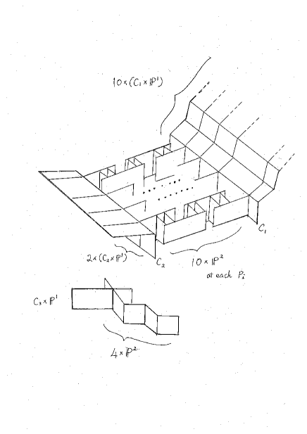
Figure 10. Exceptional divisors for Example 6.11

7. Cohomology of product and quotient varieties

In this section, we consider threefolds constructed by taking finite quotients of the product of a diagonal curve and a diagonal surface. We describe their cohomology over $\overline{k}$.

Let $Q_{1}=(w_{0},w_{1},w_{2},w_{3})$ and $Q_{2}=(v_{0},v_{1},v_{2})$. Let $S$ be a weighted diagonal surface of degree $d$ in $\mathbb{P}^{3}(Q_{1})$ and $C$ be a weighted diagonal curve of degree $e$ in $\mathbb{P}^{2}(Q_{2})$. (As we work over $\overline{k}$, $S$ and $C$ may be chosen to be of Fermat type.) Write

$$\begin{array}[]{l}\Gamma_{S}=\mu_{d/w_{0}}\times\cdots\times\mu_{d/w_{3}}/(\mbox{diagonal elements})\\ \Gamma_{C}=\mu_{e/v_{0}}\times\mu_{e/v_{1}}\times\mu_{e/v_{2}}/(\mbox{diagonal elements}).\end{array}$$

In Section 2, we find the following decomposition:

(7.1) $$\begin{array}[]{ll}H^{2}(S,\mathbb{Q}_{\ell})&\cong V(0)\oplus\bigoplus_{\mathbf{a}\in\mathfrak{A}_{S}}V(\mathbf{a})\\ H^{1}(C,\mathbb{Q}_{\ell})&\cong\bigoplus_{\mathbf{b}\in\mathfrak{A}_{C}}V(\mathbf{b})\end{array}$$

where

$$\begin{array}[]{l}\mathfrak{A}_{S}:=\biggl{\{}\mathbf{a}=(a_{0},a_{1},a_{2},a_{3})\,|\,a_{i}\in(w_{i}\mathbb{Z}/d\mathbb{Z}),a_{i}\neq 0,\sum_{i=0}^{3}a_{i}\equiv 0\pmod{d}\biggr{\}}\\ \mathfrak{A}_{C}:=\biggl{\{}\mathbf{b}=(b_{0},b_{1},b_{2})\,|\,b_{i}\in(v_{i}\mathbb{Z}/e\mathbb{Z}),b_{i}\neq 0,\sum_{i=0}^{2}b_{i}\equiv 0\pmod{e}\biggr{\}}.\end{array}$$

and

$$\begin{array}[]{l}V(\mathbf{a})=\{v\in H^{2}_{prim}(S,\mathbb{Q}_{\ell})\mid\gamma^{*}(v)={\zeta}_{0}^{a_{1}}{\zeta}_{1}^{a_{1}}{\zeta}_{2}^{a_{2}}{\zeta}_{3}^{a_{3}}v,\ \forall\gamma=({\zeta}_{0},{\zeta}_{1},{\zeta}_{2},{\zeta}_{3})\in\Gamma_{S}\}\\ V(\mathbf{b})=\{v\in H^{1}(C,\mathbb{Q}_{\ell})\mid\gamma^{*}(v)={\xi}_{0}^{b_{0}}{\xi}_{1}^{b_{0}}{\xi}_{2}^{b_{2}}v,\ \forall\xi=({\xi}_{0},{\xi}_{1},{\xi}_{2})\in\Gamma_{C}\}.\end{array}$$

Lemma 7.1.

Let $S$ be a weighted diagonal surface and $C$ be a weighted diagonal curve. Write $Y=S\times C$. Then the cohomology of $Y$ is described as follows:

$$\begin{array}[]{ll}H^{0}(Y,\mathbb{Q}_{\ell})=&H^{0}(S)\otimes H^{0}(C)\cong\mathbb{Q}_{\ell}\\ H^{1}(Y,\mathbb{Q}_{\ell})=&H^{0}(S)\otimes H^{1}(C)\cong H^{1}(C)\\ H^{2}(Y,\mathbb{Q}_{\ell})=&H^{2}(S)\otimes H^{0}(C)\oplus H^{0}(S)\otimes H^{2}(C)\cong H^{2}(S)\oplus\mathbb{Q}_{\ell}(-1)\\ H^{3}(Y,\mathbb{Q}_{\ell})=&H^{2}(S)\otimes H^{1}(C)\\ H^{4}(Y,\mathbb{Q}_{\ell})=&H^{2}(S)(-1)\oplus\mathbb{Q}_{\ell}(-2)\\ H^{5}(Y,\mathbb{Q}_{\ell})=&H^{4}(S)\otimes H^{1}(C)\cong H^{1}(C)(-2)\\ H^{6}(Y,\mathbb{Q}_{\ell})=&H^{4}(S)\otimes H^{2}(C)\cong\mathbb{Q}_{\ell}(-3)\end{array}$$

Proof.

This follows from the Künneth formula (2.2) in Section 2 and the fact that $H^{1}(S,\mathbb{Q}_{\ell})=H^{3}(S,\mathbb{Q}_{\ell})=0$ for a weighted diagonal surface $S$. Also note that $H^{2}(C)=\mathbb{Q}_{\ell}(-1)$ and $H^{4}(S)=\mathbb{Q}_{\ell}(-2)$. ∎

For $Y=S\times C$, let $\Gamma_{Y}$ be a subgroup of $\Gamma_{S}\times\Gamma_{C}$ acting on $Y$ and consisting of elements of the form

$$\boldsymbol{\gamma}=(({\zeta}_{0},{\zeta}_{1},{\zeta}_{2},{\zeta}_{3}),({\xi}_{0},{\xi}_{1},{\xi}_{2})).$$

Write

$$\begin{array}[]{l}\mathfrak{A}_{S}^{\Gamma}:=\{\mathbf{a}=(a_{0},a_{1},a_{2},a_{3})\in\mathfrak{A}_{S}\,|\,{\zeta}_{0}^{a_{0}}{\zeta}_{1}^{a_{1}}{\zeta}_{2}^{a_{2}}{\zeta}_{3}^{a_{3}}=1,\ \forall\boldsymbol{\gamma}\in\Gamma_{Y}\}\\ \mathfrak{A}_{C}^{\Gamma}:=\{\mathbf{b}=(b_{0},b_{1},b_{2})\in\mathfrak{A}_{C}\,|\,{\xi}_{0}^{b_{0}}{\xi}_{1}^{b_{1}}{\xi}_{2}^{b_{2}}=1,\ \forall\boldsymbol{\gamma}\in\Gamma_{Y}\}\\ \mathfrak{A}_{X}:=\{(\mathbf{a},\mathbf{b})\in\mathfrak{A}_{S}\times\mathfrak{A}_{C}\,|\,\zeta_{0}^{a_{0}}\zeta_{1}^{a_{1}}\zeta_{2}^{a_{2}}\zeta_{3}^{a_{3}}\xi_{0}^{b_{0}}\xi_{1}^{b_{1}}\xi_{2}^{b_{2}}=1,\ \forall\boldsymbol{\gamma}\in\Gamma_{Y}\}.\end{array}$$

Proposition 7.2.

Let $S$ be a diagonal surface of degree $d$ in $\mathbb{P}^{3}(Q_{1})$ and $C$ be a diagonal curve of degree $e$ in $\mathbb{P}^{2}(Q_{2})$. Write $Y=S\times C$ and let $\Gamma_{Y}$ be a subgroup of $\Gamma_{S}\times\Gamma_{C}$ as above. Assume $(p,\#\Gamma_{Y})=1$ and write $X=Y/\Gamma_{Y}$. Then the cohomology of $X$ is described as follows:

$$\begin{array}[]{ll}H^{0}(X,\mathbb{Q}_{\ell})=&\mathbb{Q}_{\ell}\\ H^{1}(X,\mathbb{Q}_{\ell})=&\bigoplus\limits_{\mathbf{b}\in\mathfrak{A}_{C}^{\Gamma}}V(\mathbf{b})\\ H^{2}(X,\mathbb{Q}_{\ell})=&V(0)\oplus\bigoplus\limits_{\mathbf{a}\in\mathfrak{A}_{S}^{\Gamma}}V(\mathbf{a})\oplus\mathbb{Q}_{\ell}(-1)\\ H^{3}(X,\mathbb{Q}_{\ell})=&\bigoplus\limits_{\mathbf{b}\in\mathfrak{A}_{C}^{\Gamma}}V(0)\otimes V(\mathbf{b})\oplus\bigoplus\limits_{(\mathbf{a},\mathbf{b})\in\mathfrak{A}_{X}}V(\mathbf{a})\otimes V(\mathbf{b})\end{array}$$

Other cohomology groups can be calculated from these by the Poincaré duality.

Proof.

Note that the actions by $\Gamma_{C}$, $\Gamma_{S}$ and $\Gamma_{Y}$ are compatible with the decomposition (2.1) of cohomology groups. By the assumption $(p,\#\Gamma_{Y})=1$ and an isomorphism (2.3) in Section 2, we have

$$\begin{array}[]{ll}H^{0}(X,\mathbb{Q}_{\ell})=&\mathbb{Q}_{\ell}\\ H^{1}(X,\mathbb{Q}_{\ell})=&H^{1}(C)^{\Gamma_{Y}}\\ H^{2}(X,\mathbb{Q}_{\ell})=&H^{2}(S)^{\Gamma_{Y}}\oplus\mathbb{Q}_{\ell}(-1)\\ H^{3}(X,\mathbb{Q}_{\ell})=&(H^{2}(S)\otimes H^{1}(C))^{\Gamma_{Y}}.\end{array}$$

First we consider $(H^{2}(S)\otimes H^{1}(C))^{\Gamma_{Y}}$. As $V(\mathbf{a})$ and $V(\mathbf{b})$ are subspaces of dimension one, there exist non-zero vectors $u_{1}\in V(\mathbf{a})$ and $u_{2}\in V(\mathbf{b})$ forming a basis for them respectively. Then $u_{1}\otimes u_{2}$ is a basis for $V(\mathbf{a})\otimes V(\mathbf{b})$. Since $\Gamma_{Y}$ is a subgroup of $\Gamma_{S}\times\Gamma_{C}$, it acts on $Y=S\times C$ coordinate-wise. Hence $\boldsymbol{\gamma}=(({\zeta}_{0},{\zeta}_{1},{\zeta}_{2},{\zeta}_{3}),({\xi}_{0},{\xi}_{1},{\xi}_{2}))\in\Gamma_{Y}$ sends $u_{1}\otimes u_{2}\in V(\mathbf{a})\otimes V(\mathbf{b})$ to

$$\begin{array}[]{ll}\boldsymbol{\gamma}^{*}(u_{1}\otimes u_{2})&=\zeta_{0}^{a_{0}}\zeta_{1}^{a_{1}}\zeta_{2}^{a_{2}}\zeta_{3}^{a_{3}}u_{1}\otimes\xi_{0}^{b_{0}}\xi_{1}^{b_{1}}\xi_{2}^{b_{2}}u_{2}\\ &=\zeta_{0}^{a_{0}}\zeta_{1}^{a_{1}}\zeta_{2}^{a_{2}}\zeta_{3}^{a_{3}}\xi_{0}^{b_{0}}\xi_{1}^{b_{1}}\xi_{2}^{b_{2}}(u_{1}\otimes u_{2}).\end{array}$$

It follows that $V(\mathbf{a})\otimes V(\mathbf{b})$ is invariant under the $\Gamma_{Y}$-action if and only if

$$\zeta_{0}^{a_{0}}\zeta_{1}^{a_{1}}\zeta_{2}^{a_{2}}\zeta_{3}^{a_{3}}\xi_{0}^{b_{0}}\xi_{1}^{b_{1}}\xi_{2}^{b_{2}}=1$$

for all $\boldsymbol{\gamma}\in\Gamma_{Y}$. Therefore

$$(H^{2}(S)\otimes H^{1}(C))^{\Gamma_{Y}}\cong\bigoplus_{\mathbf{b}\in\mathfrak{A}_{C}^{\Gamma}}V(0)\otimes V(\mathbf{b})\oplus\bigoplus_{(\mathbf{a},\mathbf{b})\in\mathfrak{A}_{X}}V(\mathbf{a})\otimes V(\mathbf{b}).$$

Next we consider $H^{1}(C)^{\Gamma_{Y}}$. If $u_{2}\in V(\mathbf{b})$ denotes a basis for $V(\mathbf{b})$ as above, we have

$$\boldsymbol{\gamma}^{*}(u_{2})=\xi_{0}^{b_{0}}\xi_{1}^{b_{1}}\xi_{2}^{b_{2}}u_{2}.$$

Hence $\Gamma_{Y}$ fixes $V(\mathbf{b})$ if and only if $\xi_{0}^{b_{0}}\xi_{1}^{b_{1}}\xi_{2}^{b_{2}}=1$, namely, if and only if $\mathbf{b}\in\mathfrak{A}_{C}^{\Gamma}$.

The calculation of $H^{2}(S)^{\Gamma_{Y}}$ is similar to $H^{1}(C)^{\Gamma_{Y}}$. The difference is the existence of the subgroup $V(0)$ corresponding to the hyperplane section. It is fixed by the action of $\Gamma_{Y}$ and so we obtain the decomposition of $H^{2}(X,\mathbb{Q}_{\ell})$ as asserted. ∎

The cohomology of $X$ becomes simpler when $\mathfrak{A}_{C}^{\Gamma}=\emptyset$. Such a case occurs frequently: typical examples are the diagonal inductive structure and many cases of the twist map discussed in the next section. These cases have the feature described in the following Corollary.

Corollary 7.3.

The assumption and hypothesis of Proposition 7.2 remain in force. Assume that $(v_{0},e/v_{0})=1$ and that $\Gamma_{Y}$ consists of elements of the form $\boldsymbol{\gamma}=(({\zeta}_{0},{\zeta}_{1},{\zeta}_{2},{\zeta}_{3}),({\xi}_{0},1,1))$. Then the cohomology of $X$ is described as follows:

$$\begin{array}[]{ll}H^{0}(X,\mathbb{Q}_{\ell})=&\mathbb{Q}_{\ell}\\ H^{1}(X,\mathbb{Q}_{\ell})=&0\\ H^{2}(X,\mathbb{Q}_{\ell})=&V(0)\oplus\bigoplus\limits_{\mathbf{a}\in\mathfrak{A}_{S}^{\Gamma}}V(\mathbf{a})\oplus\mathbb{Q}_{\ell}(-1)\\ H^{3}(X,\mathbb{Q}_{\ell})=&\bigoplus\limits_{(\mathbf{a},\mathbf{b})\in\mathfrak{A}_{X}}V(\mathbf{a})\otimes V(\mathbf{b})\end{array}$$

Other cohomology groups can be calculated by the Poincaré duality.

Proof.

The action of $\Gamma_{Y}$ restricted to $C$ is given as $(\xi_{0},1,1)$. Hence

$$\mathfrak{A}_{C}^{\Gamma}=\{\mathbf{b}=(b_{0},b_{1},b_{2})\in\mathfrak{A}_{C}\,|\,{\xi}_{0}^{b_{0}}=1,\ \forall\xi_{0}\in\mu_{e/v_{0}}\}.$$

As $(v_{0},e/v_{0})=1$, we have $b_{0}=0$ in $v_{0}\mathbb{Z}/e\mathbb{Z}$. Since there is no such $\mathbf{b}$ in $\mathfrak{A}_{C}$ from the definition of $\mathfrak{A}_{C}$, $\mathfrak{A}_{C}^{\Gamma}=\emptyset$ and the results follows from Proposition 7.2. ∎

8. Zeta-functions of $K3$-fibered Calabi–Yau threefolds, I

In this section, we compute zeta-functions of $K3$-fibered Calabi–Yau threefolds defined earlier. All these Calabi–Yau threefolds are realized as quotient threefolds by twist maps.

Definition 8.1.

Let $K$ be a number field, ${\mathcal{O}}_{K}$ the ring of integers of $K$. Let $V$ be a smooth projective variety defined over $K$. For a prime ${\mathfrak{p}}\in\mbox{Spec}({\mathcal{O}}_{K})$, let $V_{\mathfrak{p}}$ be the reduction of $V$ modulo ${\mathfrak{p}}$ and put $q=\#({\mathcal{O}}_{K}/{\mathfrak{p}})=\mbox{Norm}(\mathfrak{p})$. The zeta-function of $V_{\mathfrak{p}}$ is defined by

$$Z(V_{\mathfrak{p}},t)=\mbox{exp}\biggl{(}\sum_{n=1}^{\infty}\frac{\#V_{\mathfrak{p}}(\mathbb{F}_{q^{n}})}{n}t^{n}\biggr{)}$$

where $t$ is an indeterminate, and $\#V_{\mathfrak{p}}(\mathbb{F}_{q^{n}})$ is the number of rational points on $V_{\mathfrak{p}}$ over $\mathbb{F}_{q^{n}}$.

It is known (Deligne [5]) that $Z(V_{\mathfrak{p}},t)$ is a rational function and indeed has the form

$$Z(V_{\mathfrak{p}},t)=\prod_{i=0}^{2\dim(V_{\mathfrak{p}})}P_{i}(V_{\mathfrak{p}},t)^{(-1)^{i+1}}$$

where $P_{i}(V_{\mathfrak{p}},t)$ is the characteristic polynomial of the endomorphism on the $i$–th étale cohomology group $H^{i}(V_{\mathfrak{p}},\mathbb{Q}_{\ell})$ induced by the Frobenius morphism $\mbox{Frob}_{q}$ on $V_{\mathfrak{p}}$.

$$P_{i}(V_{\mathfrak{p}},t)=\det(1-\mbox{Frob}_{q}^{*}t\mid H^{i}(V_{\mathfrak{p}},\mathbb{Q}_{\ell})).$$

One knows that $P_{i}(V_{\mathfrak{p}},t)$ is a polynomial with integer coefficients of degree equal to the $i$–th Betti number $B_{i}(V_{\mathfrak{p}})$ and its reciprocal roots have the absolute value $q^{1/2}$.

Our goal of this section is to determine the zeta-function of Calabi–Yau varieties constructed in Section 5. Since our Calabi–Yau varieties are quotients of products of lower dimensional varieties. For instance, for Calabi–Yau threefolds $X$, they are quotients of products $S\times C$ of surfaces $S$ and curves $C$. Then the eigenvalues of the Frobenius for $X$ are given by products of the eigenvalues of the Frobenius on the components. For dimensions $1$ and $2$ Calabi–Yau varieties discussed in the section 5, the zeta-functions have been determined by Goto [8, 9].

To describe the eigenvalues and the zeta-functions, we need to introduce weighted Jacobi sums. The reader is referred to Gouvêa and Yui [11] for Jacobi sums and their properties relevant to our discussions.

Definition 8.2.

Let $\mathbb{L}=\mathbb{Q}(e^{2\pi\sqrt{-1}/d})$ be the $d$–th cyclotomic field over $\mathbb{Q}$, ${\mathcal{O}}_{\mathbb{L}}$ the ring of integers of $\mathbb{L}$. Let ${\mathfrak{p}}\in\mbox{Spec}({\mathcal{O}}_{\mathbb{L}})$. For every $x\in{\mathcal{O}}_{\mathbb{L}}$ relatively prime to ${\mathfrak{p}}$, let $\chi_{\mathfrak{p}}(x\ \mbox{mod}\,{\mathfrak{p}})=(\frac{x}{\mathfrak{p}})$ be the $d$–th power residue symbol on $\mathbb{L}$. If $x\equiv 0\pmod{\mathfrak{p}}$, we put $\chi_{\mathfrak{p}}(x\ \mbox{mod}\,{\mathfrak{p}})=0$. Let $(w_{0},w_{1},w_{2},\cdots,w_{n+1})$ be a weight. Define the set

$$\begin{split}&{\mathfrak{A}}_{d}(w_{0},w_{1},\cdots,w_{n+1})\\ &:=\biggl{\{}{\mathbf{a}}=(a_{0},a_{1},\cdots,a_{n+1})\,|\,a_{i}\in(w_{i}\mathbb{Z}/d\mathbb{Z}),a_{i}\neq 0,\sum_{i=0}^{n+1}a_{i}\equiv 0\pmod{d}\biggr{\}}.\end{split}$$

For each ${\mathbf{a}}\in{\mathfrak{A}}_{d}(w_{0},w_{1},\cdots,w_{n+1})$, the Jacobi sum is defined by

$$j_{\mathfrak{p}}(\mathbf{a})=j_{\mathfrak{p}}(a_{0},a_{1},\cdots,a_{n+1}):=(-1)^{n}\sum\chi_{\mathfrak{p}}(v_{1})^{a_{1}}\chi_{\mathfrak{p}}(v_{2})^{a_{2}}\cdots\chi_{\mathfrak{p}}(v_{n+1})^{a_{n+1}}$$

where the sum is taken over $(v_{1},v_{2},\cdots,v_{n+1})\in({\mathcal{O}}_{\mathbb{L}}/{\mathfrak{p}})^{\times}\times\cdots\times({\mathcal{O}}_{\mathbb{L}}/{\mathfrak{p}})^{\times}$ subject to the linear relation $1+v_{1}+v_{2}+\cdots+v_{n+1}\equiv 0\pmod{\mathfrak{p}}$.

Jacobi sums are elements of ${\mathcal{O}}_{\mathbb{L}}$ with complex absolute value equal to $q^{n/2}$ where $q=\mid\mbox{Norm}\,{\mathfrak{p}}\mid\equiv 1\pmod{d}$.

The Jacobi sums defined above are particularly useful when we describe zeta-functions of varieties over some extensions of $\mathbb{L}=\mathbb{Q}(e^{2\pi\sqrt{-1}/d})$. To discuss zeta-functions of varieties over $\mathbb{Q}$, however, we also need Jacobi sums of finite fields.

Definition 8.3.

Let $\mathbb{F}_{q}$ be a finite field of $q$ elements. Let $d$ be a positive integer. Assume that $q\equiv 1\pmod{d}$. Fix a character $\chi:\mathbb{F}_{q}^{\times}\longrightarrow\mathbb{C}^{\times}$ of exact order $d$. Define the set ${\mathfrak{A}}_{d}(w_{0},w_{1},\cdots,w_{n+1})$ as in Definition 8.2. The Jacobi sum of $\mathbb{F}_{q}$ associated with $\mathbf{a}=(a_{0},\cdots,a_{n+1})$ is defined to be

$$j_{q}(\mathbf{a}):=(-1)^{n}\sum{\chi}^{a_{1}}(v_{1})\cdots\chi^{a_{n+1}}(v_{n+1})$$

where the sum is taken over all $v_{i}\in\mathbb{F}_{q}^{\times}$ satisfying $1+v_{1}+\cdots+v_{n+1}=0$.

Jacobi sums $j_{q}(\mathbf{a})$ have absolute value $q^{n/2}$. These Jacobi sums are used to describe zeta-functions of varieties over $\mathbb{Q}$ reduced modulo $p$.

8.1. Zeta-functions of elliptic curves and $K3$ surfaces

Lemma 8.1.

Let $E_{i}$ $(i=1,2,3)$ be elliptic curves listed in Table 1. Assume that the field of definition of $E_{i}$ $(i=1,2,3)$ is a number field $K$ that contains $\mathbb{L}=\mathbb{Q}(e^{2\pi\sqrt{-1}/d})$. For $\mathfrak{p}\in\mbox{\em Spec}{\mathcal{O}}_{K}$, let $E_{i,\mathfrak{p}}$ be the reduction of $E_{i}$ modulo ${\mathfrak{p}}$. Then the zeta-function $Z(E_{i,\mathfrak{p}},t)$ has the form

$$Z(E_{i,{\mathfrak{p}}},t)=\frac{P_{1}(E_{i,{\mathfrak{p}}},t)}{(1-t)(1-qt)}$$

The polynomial $P_{1}(E_{i,{\mathfrak{p}}},t)$ is determined in Table 7.

Table 7. Polynomial $P_{1}(E_{i,{\mathfrak{p}}},t)$

$$\begin{array}[]{c|c|c|c}\hline\cr\hline\cr E_{i}&P_{1}(E_{i,\mathfrak{p}},t)&{\mathfrak{p}}&\mathbb{L}\\ \hline\cr E_{1}&(1-j_{\mathfrak{p}}(1,1,1)t)(1-j_{\mathfrak{p}}(2,2,2)t)&{\mathfrak{p}}\nmid 3&\mathbb{Q}(e^{2\pi i/3})\\ &1&{\mathfrak{p}}|3&\\ \hline\cr E_{2}&(1-j_{\mathfrak{p}}(1,1,2)t)(1-j_{\mathfrak{p}}(3,3,2)t)&{\mathfrak{p}}\nmid 4&\mathbb{Q}(e^{2\pi i/4})\\ &1&{\mathfrak{p}}|4&\\ \hline\cr E_{3}&(1-j_{\mathfrak{p}}(1,2,3)t)(1-j_{\mathfrak{p}}(5,4,3)t)&{\mathfrak{p}}\nmid 6&\mathbb{Q}(e^{2\pi i/6})\\ &1&{\mathfrak{p}}|6&\\ \hline\cr\hline\cr\end{array}$$

Proof.

$E_{i,\mathfrak{p}}$ is an elliptic curve over $\mathbb{F}_{q}$ with $q=\mid\mbox{Norm}\,{\mathfrak{p}}\mid$. As $q\equiv 1\pmod{d}$ for every $\mathfrak{p}$, each $j_{\mathfrak{p}}$ is a Jacobi sum of $\mathbb{F}_{q}$ and we can apply Weil’s method to compute $Z(E_{i,{\mathfrak{p}}},t)$. See [8] or Lemma 8.4 below. ∎

By Lemma 8.1, zeta-functions of $E_{i}$ over an extension of $\mathbb{L}$ are written in a single form throughout good reductions at $\mathfrak{p}$. When $E_{i}$ is defined over $\mathbb{Q}$, we need to divide the case according to a congruence property of a prime $p$.

Lemma 8.2.

Let $E_{i}$ $(i=1,2,3)$ be elliptic curves over $\mathbb{Q}$ listed in Table 1. For a prime $p\in\mathbb{Q}$, let $E_{i,p}$ be the reduction of $E_{i}$ modulo $p$. Then the zeta-function $Z(E_{i,p},t)$ has the form

$$Z(E_{i,p},t)=\frac{P_{1}(E_{i,p},t)}{(1-t)(1-pt)}$$

The polynomial $P_{1}(E_{i,p},t)$ is determined in Table 8.

Table 8. Polynomial $P_{1}(E_{i,p},t)$

$$\begin{array}[]{c|c|l}\hline\cr\hline\cr E_{i}&P_{1}(E_{i,p},t)&p\\ \hline\cr E_{1}&(1-j_{p}(1,1,1)t)(1-j_{p}(2,2,2)t)&p\equiv 1\pmod{3}\\ &(1-\sqrt{p}t)(1+\sqrt{p}t)&p\equiv 2\pmod{3}\\ &1&p=3\\ \hline\cr E_{2}&(1-j_{p}(1,1,2)t)(1-j_{p}(3,3,2)t)&p\equiv 1\pmod{4}\\ &(1-\sqrt{p}t)(1+\sqrt{p}t)&p\equiv 3\pmod{4}\\ &1&p=2\\ \hline\cr E_{3}&(1-j_{p}(1,2,3)t)(1-j_{p}(5,4,3)t)&p\equiv 1\pmod{6}\\ &(1-\sqrt{p}t)(1+\sqrt{p}t)&p\equiv 5\pmod{6}\\ &1&p=2,3\\ \hline\cr\hline\cr\end{array}$$

Proof.

When $p\equiv 1\pmod{d}$, the situation is the same as in Lemma 8.1 and $Z(E_{i,p},t)$ can be expressed with Jacobi sums on $\mathbb{F}_{p}$.

When $p\not\equiv 1\pmod{d}$, we need to consider several extensions of the field of definition and collect more data to determine the zeta-functions. Let $n$ be the extension degree of $\mathbb{F}_{q}$ over $\mathbb{F}_{p}$.

(i) $E_{1}$ over $\mathbb{F}_{p}$ with $p\equiv 2\pmod{3}$.

(a) Let $n$ be an odd integer and $q=p^{n}$. We have $q\equiv 2\pmod{3}$ and $E_{1}$ has the same number of $\mathbb{F}_{q}$-rational points as a curve $y_{0}^{\gcd(3,q-1)}+y_{1}^{\gcd(3,q-1)}+y_{2}^{\gcd(3,q-1)}=0$, namely

$$C:\ y_{0}+y_{1}+y_{3}=0\quad\subset\mathbb{P}^{2}.$$

Clearly, $\#E_{1,p}(\mathbb{F}_{q})=\#C_{p}(\mathbb{F}_{q})=1+q$.

(b) Let $n=2m$ be an even integer and $q=p^{n}$. We have $q\equiv 1\pmod{3}$ and we can apply Weil’s algorithm to obtain

$$\#E_{1,p}(\mathbb{F}_{q})=1+q-j_{p^{2}}(1,1,1)^{m}-j_{p^{2}}(2,2,2)^{m}.$$

It follows from [1], Theorem 11.6.1 (cf. Remark 8.1) that $j_{p^{2}}(1,1,1)=j_{p^{2}}(2,2,2)=p$. Hence $\#E_{1,p}(\mathbb{F}_{q})=1+q-2p^{m}$.

Combining (a) and (b), we determine $\#E_{1,p}(\mathbb{F}_{p^{n}})=1+p^{n}-(\sqrt{p})^{n}-(-\sqrt{p})^{n}$, which gives rise to the desired formula.

(ii) $E_{2}$ over $\mathbb{F}_{p}$ with $p\equiv 3\pmod{4}$.

(a) Let $n$ be an odd integer and $q=p^{n}$. We have $q\equiv 3\pmod{4}$ and $E_{2}$ has the same number of $\mathbb{F}_{q}$-rational points as $y_{0}^{\gcd(4,q-1)}+y_{1}^{\gcd(4,q-1)}+y_{2}^{\gcd(2,q-1)}=0$, namely

$$C:\ y_{0}^{2}+y_{1}^{2}+y_{3}^{2}=0\quad\subset\mathbb{P}^{2}.$$

We see immediately that $\#E_{2,p}(\mathbb{F}_{q})=\#C_{p}(\mathbb{F}_{q})=1+q$.

(b) Let $n=2m$ be an even integer and $q=p^{n}$. We have $q\equiv 1\pmod{4}$ and

$$\#E_{2,p}(\mathbb{F}_{q})=1+q-j_{p^{2}}(1,1,2)^{m}-j_{p^{2}}(3,3,2)^{m}.$$

By [1], Theorem 11.6.1 again, we see $j_{p^{2}}(1,1,2)=j_{p^{2}}(3,3,2)=p$. Hence $\#E_{2,p}(\mathbb{F}_{q})=1+q-2p^{m}$.

Combining (a) and (b), we determine $\#E_{2,p}(\mathbb{F}_{p^{n}})=1+p^{n}-(\sqrt{p})^{n}-(-\sqrt{p})^{n}$.

(iii) $E_{3}$ over $\mathbb{F}_{p}$ with $p\equiv 5\pmod{6}$.

Similarly as above, we see that $\#E_{3,p}(\mathbb{F}_{p^{n}})=1+p^{n}-(\sqrt{p})^{n}-(-\sqrt{p})^{n}$ and obtain the polynomial $P_{1}(E_{3,p},t)$ as claimed. ∎

Remark 8.1.

Let $m$ be a positive integer and $p$ be a prime such that $p^{r}\equiv-1\pmod{m}$ for some $r$. Write $q=p^{2r}$ and let $\chi$ be a character of $\mathbb{F}_{q}$ of order $m$. Denote by $G_{2r}(\chi)$ the Gauss sum over $\mathbb{F}_{q}$ associated with $\chi$. Then Theorem 11.6.1 of [1] states that

$$p^{-r}G_{2r}(\chi)=\begin{cases}1&\mbox{ if }p=2\\ (-1)^{\frac{p^{r}+1}{m}}&\mbox{ if }p>2\end{cases}$$

Next we calculate the zeta-functions of $K3$ surfaces and discuss their decomposition into algebraic and transcendental parts.

Definition 8.4.

Let $Y$ be a $K3$ surface over $k=\mathbb{F}_{q}$. Let $A(Y)$ be the subspace of elements in $H^{2}(Y_{\overline{k}},\mathbb{Q}_{\ell}(1))$ that are invariant under the action of $\mbox{Gal}(\overline{k}/k^{{}^{\prime}})$ for some finite extension $k^{{}^{\prime}}$ of $k$. Let $V(Y)$ be the orthogonal complement of $A(Y)$ in $H^{2}(Y_{\overline{k}},\mathbb{Q}_{\ell}(1))$ with respect to the cup-product. We define

$$\begin{array}[]{ll}P_{2}(S_{Y},t)&=\det(1-\mbox{Frob}_{q}^{*}qt\mid A(Y))\\ P_{2}(T_{Y},t)&=\det(1-\mbox{Frob}_{q}^{*}qt\mid V(Y))\end{array}$$

and call $P_{2}(S_{Y},t)$ (resp. $P_{2}(T_{Y},t)$) the algebraic (resp. transcendental) part of $P_{2}(Y,t)$.

Remark 8.2.

The above definition is originally due to Zarhin [25] for the ordinary case. We simply extend his definition to arbitrary $K3$ surfaces. It follows from the definition that $\mbox{Frob}_{q}^{*}$ acts on both $A(Y)$ and $V(Y)$. If the Tate conjecture is true for $Y$, then $A(Y)$ is equal to the image of $NS(Y_{\overline{k}})\otimes\mathbb{Q}_{\ell}$ in $H^{2}(Y_{\overline{k}},\mathbb{Q}_{\ell}(1))$ under the cycle class map. The subspace $V(Y)$ is then isomorphic to $V_{\ell}(Br(Y_{\overline{k}}))$. The Tate conjecture is known for $K3$ surface of finite height (cf. [19]) or when $H^{2}(Y_{\overline{k}},\mathbb{Q}_{\ell}(1))$ is spanned all by algebraic cycles (i.e., $Y$ is supersingular).

Proposition 8.3.

Let $K$ be a number field. Let $Y_{i}$ $(i=1,2,\cdots,10)$ be the $K3$ surfaces constructed in Proposition 4.1 by diagonal equations

$$y_{0}^{m_{0}}+y_{1}^{m_{1}}+y_{2}^{m_{2}}+y_{3}^{m_{3}}=0$$

of degree $d$ in $\mathbb{P}^{3}(w_{0},w_{1},w_{2},w_{3})$ over $K$. Assume that $K$ contains the $d$-th cyclotomic field $\mathbb{Q}(\zeta_{d})$. Let $\mathfrak{p}$ be a prime of $K$ not dividing $d$ and put $q=\mid\mbox{Norm}\,{\mathfrak{p}}\mid$. Then the following assertions hold.

$(a)$ $q\equiv 1\pmod{d}$ and the zeta-function $Z(Y_{i,\mathfrak{p}},t)$ has the form

$$Z(Y_{i,\mathfrak{p}},t)=\frac{1}{(1-t)P_{2}(Y_{i,\mathfrak{p}},t)(1-q^{2}t)}$$

where $P_{2}(Y_{i,\mathfrak{p}},t)$ is a polynomial of integer coefficients whose reciprocal roots have the complex absolute value $q$ and

$$P_{2}(Y_{i,\mathfrak{p}},t)=(1-qt)\prod_{{\mathbf{a}}\in{\mathfrak{A}}_{d}}(1-j_{\mathfrak{p}}({\mathbf{a}})t)$$

with ${\mathfrak{A}}_{d}={\mathfrak{A}}_{d}(w_{0},w_{1},w_{2},w_{3})$.

$(b)$ Let ${\widetilde{Y}}_{i,\mathfrak{p}}$ be the minimal resolution of $Y_{i,\mathfrak{p}}$ and let $\mathcal{E}$ denote the proper transform of $\mbox{\rm Sing}\,(\overline{Y_{i,\mathfrak{p}}})$ on ${\widetilde{Y}}_{i,\mathfrak{p}}$, where $\overline{Y_{i,\mathfrak{p}}}=Y_{i,\mathfrak{p}}\times\overline{\mathbb{F}}_{q}$. Then $\mathcal{E}$ is a scheme over $\mathbb{F}_{q}$ consisting of exceptional divisors and

$$Z({\widetilde{Y}}_{i,\mathfrak{p}},t)=\frac{Z(Y_{i,\mathfrak{p}},t)}{P_{2}(\mathcal{E},t)}=\frac{1}{(1-t)P_{2}(Y_{i,\mathfrak{p}},t)P_{2}(\mathcal{E},t)(1-q^{2}t)}.$$

In particular, $P_{2}({\widetilde{Y}}_{i,\mathfrak{p}},t)=P_{2}(Y_{i,\mathfrak{p}},t)P_{2}(\mathcal{E},t)$.

$(c)$ $P_{2}({\widetilde{Y}}_{i,\mathfrak{p}},t)$ factors over $\mathbb{Z}$ as follows:

$$P_{2}({\widetilde{Y}}_{i,\mathfrak{p}},s)=P_{2}(S_{{\widetilde{Y}}_{i,\mathfrak{p}}},t)P_{2}(T_{{\widetilde{Y}}_{i,\mathfrak{p}}},t).$$

Here if $p$ is a rational prime such that $\mathfrak{p}\cap\mathbb{Z}=(p)$, then

$$P_{2}(T_{{\widetilde{Y}}_{i,\mathfrak{p}}},t)=\begin{cases}1&\mbox{ if $p^{r}\equiv-1\pmod{d}$ for some $r\in\mathbb{N}$ }\\ \prod_{{\mathbf{a}}\in\mathcal{M}_{Q}}(1-j_{\mathfrak{p}}({\mathbf{a}})t)&\mbox{ otherwise}\end{cases}$$

where $\mathcal{M}_{Q}$ is the weight motive of $Y_{i,\mathfrak{p}}$, i.e. the $(\mathbb{Z}/d\mathbb{Z})^{\times}$-orbit of ${\mathbf{a}}=(w_{0},w_{1},w_{2},w_{3})$ in ${\mathfrak{A}}_{d}$.

Proof.

(a) Since $K$ contains $\mathbb{Q}(\zeta_{d})$, we have $q\equiv 1\pmod{d}$ for every prime $\mathfrak{p}$. As $Y_{i}$ is a weighted diagonal surface over $\mathbb{F}_{q}$, $Z(Y_{i,\mathfrak{p}},t)$ can be computed by Weil’s classical method (see [8]).

(b) Each singular point in $\mbox{Sing}\,(\overline{Y_{i,\mathfrak{p}}})$ may not be defined over $\mathbb{F}_{q}$, but the subscheme $\mbox{Sing}\,(\overline{Y_{i,\mathfrak{p}}})=\overline{Y_{i,\mathfrak{p}}}\cap\mbox{Sing}\,(\mathbb{P}^{3}(Q))$ is defined over $\mathbb{F}_{q}$. Since $\mbox{Sing}\,(\mathbb{P}^{3}(Q))$ is defined over $\mathbb{F}_{q}$ and an embedded resolution exists for $\overline{Y_{i,\mathfrak{p}}}$, the resolution ${\widetilde{Y}}_{i,\mathfrak{p}}$ and a subscheme $\mathcal{E}$ are defined over $\mathbb{F}_{q}$. As $Y_{i,\mathfrak{p}}$ has only cyclic quotient singularities, $\mathcal{E}$ consists of rational lines. Hence $P_{1}(\mathcal{E},t)=1$ and $Z({\widetilde{Y}}_{i,\mathfrak{p}},t)$ has the asserted form.

(c) Since $Y_{i,\mathfrak{p}}$ is a weighted diagonal surface, the Tate conjecture holds for ${\widetilde{Y}}_{i,\mathfrak{p}}$ over $\mathbb{F}_{q}$ (cf. [8]) and its supersingularity is dependent on $p$. (Note that $\mathfrak{p}\nmid d$ implies $p\nmid d$.) As ${\widetilde{Y}}_{i,\mathfrak{p}}$ is a $K3$ surface, it is known that ${\widetilde{Y}}_{i,\mathfrak{p}}$ is supersingular if and only if $p^{r}\equiv-1\pmod{d}$ for some positive integer $r$ (see [10]). When ${\widetilde{Y}}_{i,\mathfrak{p}}$ is supersingular, all cycles are algebraic and hence $P_{2}(T_{{\widetilde{Y}}_{i,\mathfrak{p}}},t)=1$; otherwise, the weight motive $\mathcal{M}_{Q}$ corresponds to the transcendental cycles. Therefore $P_{2}(T_{{\widetilde{Y}}_{i,\mathfrak{p}}},t)$ has the form as we claim. ∎

Remark 8.3.

Since we assume $K\supset\mathbb{Q}(\zeta_{d})$, the congruence $q\equiv 1\pmod{d}$ holds for every prime $\mathfrak{p}$. If we remove this assumption, it may happen that $q\not\equiv 1\pmod{d}$ for some classes of $\mathfrak{p}$. In this case, the number of $\mathcal{O}_{K}/\mathfrak{p}$-rational points on $Y_{\mathfrak{p}}$ is the same as that of

$$y_{0}^{\gcd(m_{0},q-1)}+y_{1}^{\gcd(m_{1},q-1)}+y_{2}^{\gcd(m_{2},q-1)}+y_{3}^{\gcd(m_{3},q-1)}=0.$$

The degree, say $d^{{}^{\prime}}$, of this surface now satisfies $q\equiv 1\pmod{d^{{}^{\prime}}}$ and we can express the number of rational points in terms of Jacobi sums associated with a character of order $d^{{}^{\prime}}$. If we carry out this calculation over sufficiently many finite extensions of $\mathbb{F}_{q}$, we can obtain the zeta-function of $Y$ over $\mathbb{F}_{q}$ with $q\not\equiv 1\pmod{d}$. Furthermore, this algorithm works also over a finite prime field $\mathbb{F}_{p}$. This is what one can do in general to compute the $L$-series of $Y$ over $\mathbb{Q}$.

Remark 8.4.

It depends on the prime $(p)=\mathfrak{p}\cap\mathbb{Z}$ whether or not ${\widetilde{Y}}_{i,\mathfrak{p}}$ is supersingular. The above condition for a supersingular prime $p$ can be phrased as follows: let $\zeta_{d}=e^{2\pi i/d}$ and write $\mathbb{L}=\mathbb{Q}(\zeta_{d})$ for the $d$-th cyclotomic field over $\mathbb{Q}$. Choose a prime $\wp\in\mbox{Spec}({\mathcal{O}}_{\mathbb{L}})$ over $p$ and assume $\wp\nmid d$. Then $\wp$ is unramified in $\mathbb{L}/\mathbb{Q}$, so that the inertia group of $\wp$ is trivial. Hence its decomposition group, $Z_{\wp}$, is isomorphic to $\mbox{Gal}(\mathbb{F}_{q}/\mathbb{F}_{p})$, where $\mathbb{F}_{q}\cong{\mathcal{O}}_{\mathbb{L}}/\wp$ and $q=p^{f}$. Let $\sigma_{F}$ be the Frobenius automorphism that generates $\mbox{Gal}(\mathbb{F}_{q}/\mathbb{F}_{p})$. Then $Z_{\wp}$ is generated by $\sigma_{F}$ and it acts on $\mathbb{L}$ as $\sigma_{F}(\zeta_{d})=\zeta_{d}^{p}$ of order $f$. When $p^{r}\equiv-1\pmod{d}$, $\sigma_{F}^{r}$ acts on $\mathbb{Q}(\zeta_{d})$ as

$$\sigma_{F}^{r}(\zeta_{d})=\zeta_{d}^{p^{r}}=\zeta_{d}^{-1}=\overline{\zeta_{d}}.$$

In other words, $Z_{\wp}$ contains the complex conjugate map restricted to $\mathbb{Q}(\zeta_{d})$. The converse is also true. Therefore ${\widetilde{Y}}_{i,\mathfrak{p}}$ is supersingular if and only if $Z_{\wp}$ contains the complex conjugate.

Next we deal with quasi-diagonal surfaces; threefolds will be discussed in the next section.

Lemma 8.4.

Let $k=\mathbb{F}_{q}$ be a finite field of $q$ elements. Let $m_{1},\cdots,m_{r}$ be $r$ positive integers such that $q\equiv 1\pmod{m_{i}}$ for $1\leq i\leq r$. Write $W_{k}$ be an affine variety in $\mathbb{A}^{r}_{k}$ defined by the equation

$$b_{0}+b_{1}x_{1}^{m_{1}}+\cdots+b_{r}x_{r}^{m_{r}}=0\quad\subset\mathbb{A}^{r}_{k}$$

with $b_{i}\in k^{\times}$ $(0\leq i\leq r)$. Define

$$\begin{array}[]{l}M=\mbox{\em lcm}\,(m_{1},\cdots,m_{r})\\ M_{i}=M/m_{i}\end{array}$$

for $1\leq i\leq r$. Assume $q\equiv 1\pmod{M}$. Fix a character, $\chi$, of $k^{\times}$ of exact order $M$. Let $N(W)$ denote the number of $k$-rational points on $W_{k}$. Then

$$N(W)=q^{r-1}+\sum_{\mathbf{a}\in\mathfrak{A}_{0}}{\mathcal{J}}(\mathbf{b},\mathbf{a})$$

where

$$\begin{array}[]{l}\mathbf{b}=(b_{0},\cdots,b_{r})\\ \mathfrak{A}_{0}=\biggl{\{}\mathbf{a}=(a_{0},\cdots,a_{r})\Big{|}\ \begin{array}[]{l}a_{i}\in M_{i}\mathbb{Z}/M\mathbb{Z},\ a_{i}\neq 0\ (1\leq i\leq r),\ a_{0}\in\mathbb{Z}/M\mathbb{Z}\\ \sum_{i=0}^{r}a_{i}=0\end{array}\biggr{\}}\\ j(\mathbf{a})=\sum_{\begin{subarray}{c}v_{i}\in k^{\times}\,(1\leq i\leq r)\\ 1+v_{1}+\cdots+v_{r}=0\end{subarray}}{\chi}^{a_{1}}(v_{1})\cdots{\chi}^{a_{r}}(v_{r})\\ {\mathcal{J}}(\mathbf{b},\mathbf{a})=\chi^{-1}(b_{0}^{a_{0}}\cdots b_{r}^{a_{r}})j(\mathbf{a})\end{array}$$

Proof.

See [14], Chap. 8. ∎

Proposition 8.5.

Let $Y$ be a quasi-diagonal surface over $\mathbb{F}_{q}$ defined by an equation

$$y_{0}^{m_{0}}y_{1}+y_{1}^{m_{1}}+y_{2}^{m_{2}}+y_{3}^{m_{3}}=0$$

in $\mathbb{P}^{3}(w_{0},w_{1},w_{2},w_{3})$ of degree $d$, where $d=w_{0}m_{0}+w_{1}=w_{1}m_{1}=w_{2}m_{2}=w_{3}m_{3}$. Write

$$\begin{array}[]{l}M=\mbox{\em lcm}\,(m_{0},m_{2},m_{3})\\ M_{i}=M/m_{i}\qquad(i=0,2,3)\end{array}$$

and assume $q\equiv 1\pmod{M}$. Fix a character, $\chi$, of $k^{\times}$ of exact order $M$. Then the zeta-function of $Y$ has the form

$$Z(Y,t)=\frac{1}{(1-t)P_{2}(Y,t)(1-q^{2}t)}$$

where

$$P_{2}(Y,t)=(1-qt)\prod_{a\in\mathfrak{L}}(1-q\chi^{aM_{3}}(-1)t)\prod_{{\mathbf{a}}\in{\mathfrak{A}_{Y}}}(1-j_{\mathfrak{p}}({\mathbf{a}})t)$$

$$\mathfrak{L}=\{a\in\mathbb{Z}\mid 0<a<m_{3},\ w_{3}a\equiv 0\pmod{w_{2}}\}$$

(8.3) $$\mathfrak{A}_{Y}=\biggl{\{}{\mathbf{a}}=(a_{0},a_{1},a_{2},a_{3})\Big{|}\begin{array}[]{l}a_{1}\in\mathbb{Z}/M\mathbb{Z},\ a_{i}\in M_{i}\mathbb{Z}/M\mathbb{Z}\ (i=0,2,3),\\ a_{i}\neq 0\ (0\leq i\leq 3),\ \sum_{i=0}^{3}a_{i}=0\ \text{\em and }\ a_{0}+m_{1}a_{1}=0\end{array}\biggr{\}}$$

Proof.

Here we give an outline and cohomological explanation of the proof. A more detailed and combinatorial account of it (in the case of threefolds) may be found in Theorem 9.3.

Note first that $Y$ is a Delsarte surface with matrix

$$\left[\begin{array}[]{cccc}m_{0}&1&0&0\\ 0&m_{1}&0&0\\ 0&0&m_{2}&0\\ 0&0&0&m_{3}\end{array}\right].$$

The zeta-functions of such quasi-diagonal surfaces are computed in [9] by a combinatorial argument. The main idea there is to split the surface $Y$ according to $y_{1}=0$ or $y_{1}\neq 0$. The subset corresponding to $y_{1}=0$ consists of $r=d/\mbox{lcm}\,(w_{2},w_{3})$ lines and this gives rise to a factor $\prod_{a\in\mathfrak{L}}(1-q\chi^{aM_{3}}(-1)t)$ of $P_{2}(Y,t)$. The other factor of it comes from the diagonal surface of degree $M$. As described in [10], $Y$ is covered by the diagonal surface $F$ of degree $m_{0}m_{1}m_{2}m_{3}$ and there is a group action $\Gamma$ on $F$ so that $Y$ is birational to $F/\Gamma$. Computing the cohomology of $F/\Gamma$, we obtain the factor $\prod_{{\mathbf{a}}\in{\mathfrak{A}}}(1-j_{\mathfrak{p}}({\mathbf{a}})t)$ of $P_{2}(Y,t)$. ∎

Remark 8.5.

In general, the modulus $M$ above is different from the degree $d$ of the surface. Proposition 8.5 shows that the character set $\mathfrak{A}$ of a quasi-diagonal surface can be embedded in ${\mathfrak{A}}_{M}(1,1,1,1)$.

Corollary 8.6.

Let $Y$ be a quasi-diagonal surface over a number field $K$ defined by an equation

$$y_{0}^{m_{0}}y_{1}+y_{1}^{m_{1}}+y_{2}^{m_{2}}+y_{3}^{m_{3}}=0\ \subset\mathbb{P}^{3}(w_{0},w_{1},w_{2},w_{3}).$$

Assume that $K$ contains the $M$-th cyclotomic field $\mathbb{Q}(\zeta_{M})$. Let $\mathfrak{p}$ be a prime of $K$ not dividing $d$. Then the assertions $(a)$, $(b)$ and $(c)$ of Proposition 8.3 hold for $Y_{\mathfrak{p}}$ if we replace $d$ by $M$.

Example 8.7.

Let $Y_{11}$ be the $K3$ surface over $K$ constructed in Proposition 4.1:

$$Y_{11}:\ y_{0}^{12}y_{1}+y_{1}^{11}+y_{2}^{3}+y_{3}^{2}=0\subset\mathbb{P}^{3}(5,6,22,33).$$

For the values defined in Proposition 8.5, we find $M=12$ and $r=1$. If $\mathfrak{p}\nmid 2\cdot 3\cdot 5\cdot 11$, then the zeta-function $Z(Y_{11,\mathfrak{p}},t)$ has the form

$$Z(Y_{11,\mathfrak{p}},t)=\frac{1}{(1-t)P_{2}(Y_{11,\mathfrak{p}},t)(1-q^{2}t)}$$

where $P_{2}(Y_{11,\mathfrak{p}},t)$ is a polynomial of degree $5$ and decomposed as

$$P_{2}(Y_{11,\mathfrak{p}},t)=(1-qt)\prod_{{\mathbf{a}}\in{\mathfrak{A}}_{Y_{11}}}(1-j_{\mathfrak{p}}({\mathbf{a}})t)$$

with ${\mathfrak{A}}_{Y_{11}}=\{(1,1,4,6),(5,5,8,6),(7,7,4,6),(11,11,8,6)\}\subset{\mathfrak{A}}_{12}(1,1,1,1)$. Furthermore, if $Y_{11,\mathfrak{p}}$ is not supersingular, then

$$P_{2}(T_{Y_{11,\mathfrak{p}}},t)=\prod_{{\mathbf{a}}\in{\mathfrak{A}}_{Y_{11}}}(1-j_{\mathfrak{p}}({\mathbf{a}})t).$$

9. Zeta-functions of $K3$-fibered Calabi–Yau threefolds, II

Now we calculate the zeta-functions of Calabi–Yau threefolds. In order to have a simple exposition, we slightly raise the field of definition and express the zeta-function in a single form (independent of the choice of prime reduction).

As we noted in Section 2, we may bring in non-trivial coefficients $c_{i}$ to the defining equations of our hypersurfaces. The geometry will be the same, but the arithmetic will be different. We will give more details about the differences in a subsequent paper.

We begin with some notations to describe singular loci and resolution of singularities for our threefolds.

Definition 9.1.

Let $X$ be a weighted hypersurface in $\mathbb{P}^{4}(w_{0},w_{1},w_{2},w_{3},w_{4})$ over $k$ defined by $f=0$. Let $I_{1}$ be a set of indecies which parameterizes one-dimensional singular loci of $X$, namely

$$I_{1}=\{\mathbf{i}=(i,j,k)\mid\gcd(w_{i},w_{j},w_{k})\geq 2\}.$$

For each $\mathbf{i}=(i,j,k)$, write $\hat{\mathbf{i}}=\{0,1,2,3,4\}\setminus\{i,j,k\}$ and let $C_{\mathbf{i}}$ be a subscheme of $X$ over $k$ defined by

$$C_{\mathbf{i}}:\ f=0\mbox{ and }x_{h}=0\ (h\in\hat{\mathbf{i}}).$$

Similarly, let $I_{0}$ be a set of indecies which parameterizes zero-dimensional singular loci of $X$, namely

$$I_{0}=\{\mathbf{j}=(i,j)\mid\gcd(w_{i},w_{j})\geq 2\}.$$

For each $\mathbf{j}=(i,j)$, write $\hat{\mathbf{j}}=\{0,1,2,3,4\}\setminus\{i,j\}$ and let $P_{\mathbf{j}}$ be a subscheme of $X$ over $k$ defined by

$$P_{\mathbf{j}}:\ f=0\mbox{ and }x_{h}=0\ (h\in\hat{\mathbf{j}}).$$

Finally, for the case of quasi-diagonal hypersurfaces, we put

$$P_{0}:=(1:0:0:0:0).$$

In most cases, $C_{\mathbf{i}}$ are irreducible (i.e. varieties over $k$) and $P_{\mathbf{j}}$ are reducible. As a scheme, $P_{\mathbf{j}}$ is defined over $k$; but, if we decompose it as a set of points, each point may not be defined over $k$.

It follows from the discussion of Section 5 that if $X$ is a weighted diagonal hypersurface, then $\mbox{Sing}\,(X)$ is a scheme over $k$ and we have

$$\mbox{Sing}\,(X)=\bigcup_{\mathbf{i}\in I_{1}}C_{\mathbf{i}}\cup\bigcup_{\mathbf{j}\in I_{0}}P_{\mathbf{j}}.$$

Lemma 9.1.

Let $X$ be a quasi-smooth weighted hypersurface in $\mathbb{P}^{4}(Q)$ over $K$. Let $\mathfrak{p}$ be a prime of $K$ and $X_{\mathfrak{p}}$ be the reduction of $X$ modulo $\mathfrak{p}$. Put $q=\#(\mathcal{O}_{K}/\mathfrak{p})$. Assume that $X_{\mathfrak{p}}$ is quasi-smooth. Then there exists a crepant resolution ${\widetilde{X}}_{\mathfrak{p}}$ of $X_{\mathfrak{p}}$ that is obtained by applying a partial toroidal desingularization to $\mathbb{P}^{4}(Q)$. Let $\widetilde{C}_{\mathbf{i}}$ (resp. $\widetilde{P}_{\mathbf{j}}$) be the strict transform of $C_{\mathbf{i}}$ (resp. $P_{\mathbf{j}}$) with respect to ${\widetilde{X}}_{\mathfrak{p}}\longrightarrow X_{\mathfrak{p}}$. Write $\widetilde{C}_{\mathbf{i}}^{\circ}$ (resp. $\widetilde{P}_{\mathbf{j}}^{\circ}$) for the open subset of $\widetilde{C}_{\mathbf{i}}$ (resp. $\widetilde{P}_{\mathbf{j}}$) defined by subtracting the proper transform of $C_{\mathbf{i}}$ (resp. $P_{\mathbf{j}}$). Then we have

$$Z(\widetilde{C}_{\mathbf{i}}^{\circ},t)=\frac{P_{1}(C_{\mathbf{i}},qt)^{n_{\mathbf{i}}}}{(1-qt)^{n_{\mathbf{i}}}(1-q^{2}t)^{n_{\mathbf{i}}}},\qquad Z(\widetilde{P}_{\mathbf{j}}^{\circ},t)=\frac{1}{P_{0}(P_{\mathbf{j}},qt)^{e_{\mathbf{j}}}P_{0}(P_{\mathbf{j}},q^{2}t)^{e_{\mathbf{j}}}}$$

where $n_{\mathbf{i}}$ is the number of ruled surfaces over ${C}_{\mathbf{i}}$ and ${e_{\mathbf{j}}}$ is the number of projective planes over ${P}_{\mathbf{j}}$.

Proof.

It follows from Lemma 6.3 that $\widetilde{C}_{\mathbf{i}}^{\circ}$ consists of $n_{\mathbf{i}}q^{\nu}N_{\nu}(C_{\mathbf{i}})$ rational points over the $\nu$-th extension of $\mathcal{O}_{K}/\mathfrak{p}$. Similarly, Lemma 6.7 implies that $\widetilde{P}_{\mathbf{j}}^{\circ}$ acquires $e_{\mathbf{j}}(q^{\nu}+q^{2\nu})$ rational points. Hence their zeta-functions are computed as above. ∎

Theorem 9.2.

Let $K$ be a number field. Let $X$ be a singular Calabi–Yau threefold over $K$ of diagonal type constructed in Section $4$ by the equation

$$z_{0}^{m_{0}}+z_{1}^{m_{1}}+z_{2}^{m_{2}}+z_{3}^{m_{3}}+z_{4}^{m_{4}}=0$$

in $\mathbb{P}^{4}(w_{0},w_{1},w_{2},w_{3},w_{4})$ of degree $d=w_{0}+\cdots+w_{4}$. Assume that $K$ contains the $d$-th cyclotomic field $\mathbb{Q}(\zeta_{d})$. Let $\mathfrak{p}$ be a prime of $K$ not dividing $d$. Write $X_{\mathfrak{p}}$ for the reduction of $X$ modulo $\mathfrak{p}$ and put $\mathbb{F}_{q}:=\mathcal{O}_{K}/\mathfrak{p}$ with $q=\mbox{\em Norm}\,{\mathfrak{p}}$. Then the following assertions hold.

$(a)$ The zeta-function $Z(X_{\mathfrak{p}},t)$ has the form

$$Z(X_{\mathfrak{p}},t)=\frac{P_{3}(X_{\mathfrak{p}},t)}{(1-t)(1-qt)(1-q^{2}t)(1-q^{3}t)}$$

where $P_{3}(X_{\mathfrak{p}},t)$ is a polynomial of integer coefficients whose reciprocal roots have the complex absolute value $q^{3/2}$ and

$$P_{3}(X_{\mathfrak{p}},t)=\prod_{{\mathbf{a}}\in{\mathfrak{A}}_{d}(Q)}(1-j_{\mathfrak{p}}({\mathbf{a}})t)$$

with ${\mathfrak{A}}_{d}(Q)={\mathfrak{A}}_{d}(w_{0},w_{1},w_{2},w_{3},w_{4})$.

$(b)$ There exists a crepant resolution ${\widetilde{X}}_{\mathfrak{p}}$ of $X_{\mathfrak{p}}$ such that ${\widetilde{X}}_{\mathfrak{p}}$ is obtained by applying a toroidal desingularization to $\mathbb{P}^{4}(Q)$ and ${\widetilde{X}}_{\mathfrak{p}}$ is a Calabi–Yau threefold over $\mathbb{F}_{q}$.

$(c)$ With the notation of $(b)$ and Lemma 9.1, we have

$$Z({\widetilde{X}}_{\mathfrak{p}},t)=\frac{P_{3}({\widetilde{X}}_{\mathfrak{p}},t)}{(1-t)P_{2}({\widetilde{X}}_{\mathfrak{p}},t)P_{4}({\widetilde{X}}_{\mathfrak{p}},t)(1-q^{3}t)}$$

with

$$P_{2}({\widetilde{X}}_{\mathfrak{p}},t) =(1-qt)\prod_{\mathbf{i}\in I_{1}}(1-qt)^{n_{\mathbf{i}}}\prod_{\mathbf{j}\in I_{0}}P_{0}(P_{\mathbf{j}},qt)^{e_{\mathbf{j}}}$$

$$P_{3}({\widetilde{X}}_{\mathfrak{p}},t) =\prod_{{\mathbf{a}}\in{\mathfrak{A}}_{d}(Q)}(1-j_{\mathfrak{p}}({\mathbf{a}})t)\prod_{\mathbf{i}\in I_{1}}P_{1}(C_{\mathbf{i}},qt)^{n_{\mathbf{i}}}$$

$$P_{4}({\widetilde{X}}_{\mathfrak{p}},t) =P_{2}({\widetilde{X}}_{\mathfrak{p}},qt)$$

Proof.

(a) Since $X_{\mathfrak{p}}$ is a weighted diagonal threefold over $\mathbb{F}_{q}$ and $q\equiv 1\pmod{d}$, $Z(X_{\mathfrak{p}},t)$ can be computed by Weil’s classical method (see [8] for details).

(b) The existence of ${\widetilde{X}}_{\mathfrak{p}}$ is proven in Lemma 9.1 and its Calabi–Yau property follows from $d=w_{0}+\cdots+w_{4}$.

(c) The assertions are deduced from Lemma 9.1 by noting that

$$P_{2}({\widetilde{X}}_{\mathfrak{p}},t) =P_{2}(X_{\mathfrak{p}},t)\prod_{\mathbf{i}\in I_{1}}P_{2}(\widetilde{C}_{\mathbf{i}}^{\circ},t)\prod_{\mathbf{j}\in I_{0}}P_{2}(\widetilde{P}_{\mathbf{j}}^{\circ},t)$$

$$P_{3}({\widetilde{X}}_{\mathfrak{p}},t) =P_{3}(X_{\mathfrak{p}},t)\prod_{\mathbf{i}\in I_{1}}P_{3}(\widetilde{C}_{\mathbf{i}}^{\circ},t)\prod_{\mathbf{j}\in I_{0}}P_{3}(\widetilde{P}_{\mathbf{j}}^{\circ},t)$$

and $P_{3}(\widetilde{P}_{\mathbf{j}}^{\circ},t)=1$. ∎

Remark 9.1.

As we noted in Remark 8.3, the assumption $K\supset\mathbb{Q}(\zeta_{d})$ enables us to have $q\equiv 1\pmod{d}$ for every prime $\mathfrak{p}$. If we relax this assumption, then we can still calculate the number of $\mathcal{O}_{K}/\mathfrak{p}$-rational points on $X_{\mathfrak{p}}$ via the threefold

$$z_{0}^{\gcd(m_{0},q-1)}+z_{1}^{\gcd(m_{1},q-1)}+z_{2}^{\gcd(m_{2},q-1)}+z_{3}^{\gcd(m_{3},q-1)}+z_{4}^{\gcd(m_{4},q-1)}=0.$$

Since the degree, $d^{{}^{\prime}}$, of this threefold satisfies $q\equiv 1\pmod{d^{{}^{\prime}}}$, we can express the number of rational points in terms of Jacobi sums. We carry out this calculation over sufficiently many finite extensions of $\mathbb{F}_{q}$ to obtain $Z(X_{\mathfrak{p}},t)$ with $q\not\equiv 1\pmod{d}$. Further, this algorithm works also over $\mathbb{F}_{p}$ and one can determine the $L$-series of $X$ over $\mathbb{Q}$ (cf. Lemma 8.2). More details of it will be discussed in a subsequent paper.

Next we discuss the quasi-diagonal threefolds. The description is almost identical with that of the diagonal case.

Theorem 9.3.

Let $X$ be a quasi-diagonal threefold over $\mathbb{F}_{q}$ defined by an equation

$$z_{0}^{m_{0}}z_{1}+z_{1}^{m_{1}}+z_{2}^{m_{2}}+z_{3}^{m_{3}}+z_{4}^{m_{4}}=0$$

in $\mathbb{P}^{4}(k_{0},k_{1},k_{2},k_{3},k_{4})$ of degree $d$, where $d=k_{0}m_{0}+k_{1}=k_{1}m_{1}=k_{2}m_{2}=k_{3}m_{3}=k_{4}m_{4}$. Let $C$ be a weighted diagonal curve of degree $d$ in $\mathbb{P}^{2}(k_{2},k_{3},k_{4})$ defined by

$$z_{2}^{m_{2}}+z_{3}^{m_{3}}+z_{4}^{m_{4}}=0.$$

Write

$$\begin{array}[]{l}M=\mbox{\em lcm}\,(m_{0},m_{2},m_{3},m_{4})\\ M_{i}=M/m_{i}\qquad(i=0,2,3,4).\end{array}$$

Let $Z(C,t)=P_{1}(C,t)/(1-t)(1-qt)$ denote the zeta-function of $C$ over $\mathbb{F}_{q}$. Assume $q\equiv 1\pmod{M}$. Then the zeta-function of $X$ has the form

$$Z(X,t)=\frac{P_{3}(X,t)}{(1-t)(1-qt)(1-q^{2}t)(1-q^{3}t)}$$

where

$$P_{3}(X,t)=P_{1}(C,qt)\prod_{{\mathbf{a}}\in{\mathfrak{A}}_{X}}(1-j_{\mathfrak{p}}({\mathbf{a}})t)$$

$$\mathfrak{A}_{X}=\biggl{\{}{\mathbf{a}}=(a_{0},\cdots,a_{4})\Big{|}\begin{array}[]{l}a_{1}\in\mathbb{Z}/M\mathbb{Z},\ a_{i}\in M_{i}\mathbb{Z}/M\mathbb{Z}\ (i=0,2,3,4),\\ a_{i}\neq 0\ (0\leq i\leq 4),\ \sum_{i=0}^{4}a_{i}=0\ \text{\em and }\ a_{0}+m_{1}a_{1}=0\end{array}\biggr{\}}$$

Remark 9.2.

The main differences of zeta-functions between diagonal and quasi-diagonal threefolds are $P_{3}(X,t)$ and the modulus for $\mathfrak{A}$. Since $M$ is often smaller than $d$, the factor of $P_{3}(X,t)$ associated with the weight motive can be smaller than that of a diagonal threefold of the same degree. Here the weight motive means the $(\mathbb{Z}/M\mathbb{Z})^{\times}$-orbit of ${\mathbf{a}}=(M_{0},M_{1},M_{2},M_{3},M_{4})$ in ${\mathfrak{A}}_{X}$ with $M_{1}:=M-M_{0}-M_{2}-M_{3}-M_{4}$. We will discuss more details about weight motives elsewhere (cf. [24]).

Proof.

Let $\overline{X}$ be the affine quasi-cone of $X$ in $\mathbb{A}^{5}$. Write $k_{\nu}$ for the extension of $k:=\mathbb{F}_{q}$ of degree $\nu$. Denote by $N_{\nu}(X)$ for the number of $k_{\nu}$-rational points on $X$. By Corollary 1.4 of [8], we have $N_{\nu}(\overline{X})=1+(q^{\nu}-1)N_{\nu}(X)$. Let $V$ be the closed subset of $X$ defined by $z_{1}=0$; i.e.

$$V:\ \ z_{2}^{m_{2}}+z_{3}^{m_{3}}+z_{4}^{m_{4}}=0\ \mbox{ with $z_{0}$ being free }\ \subset\mathbb{A}^{4}.$$

Write $U$ for the open subset $X\setminus V$:

(9.1) $$U:\ \ z_{0}^{m_{0}}z_{1}+z_{1}^{m_{1}}+z_{2}^{m_{2}}+z_{3}^{m_{3}}+z_{4}^{m_{4}}=0\ \mbox{ with $z_{1}\neq 0$ }\ \subset\mathbb{A}^{5}.$$

Then $X_{k_{\nu}}=V_{k_{\nu}}\cup U_{k_{\nu}}$ (disjoint union) for every $\nu\geq 1$. Regarding $z_{1}$ as a constant in $k_{\nu}^{\times}$, write $U(z_{1})$ for the affine hypersurface in $\mathbb{A}^{4}_{k_{\nu}}$ defined by the equation (9.1). Then for $\nu\geq 1$,

$$N_{\nu}(\overline{X})=N_{\nu}(V)+\sum_{z_{1}\in k_{\nu}^{\times}}N_{\nu}(U(z_{1})).$$

Write $P_{1}(C,t)=\prod_{i}(1-\alpha_{i}t)$. It follows from Weil’s classical results that

$$N_{\nu}(V)=q^{\nu}\bigl{\{}q^{2\nu}-(q^{\nu}-1)\sum_{i}\alpha_{i}^{\nu}\bigr{\}}.$$

Applying Lemma 8.4 to the case $r=4,\ b_{0}=z_{1}^{m_{1}},\ b_{1}=z_{1}$ and $b_{2}=b_{3}=b_{4}=1$ (and also interchanging $a_{0}$ and $a_{1}$), we find

$$N_{\nu}(U(z_{0}))=q^{3\nu}-\sum_{\mathbf{a}\in\mathfrak{A}_{0}}\chi_{\nu}^{-1}(z_{1}^{m_{1}a_{1}+a_{0}})j_{\nu}(\mathbf{a})$$

where $\chi_{\nu}$ is a non-trivial character of $k_{\nu}^{\times}$ defined by $\chi_{\nu}=\chi\circ N_{k_{\nu}/k}$, $j_{\nu}$ is the sum

$$j_{\nu}(\mathbf{a})=-\sum_{\begin{subarray}{c}v_{i}\in k_{\nu}^{\times}\,(1\leq i\leq 4)\\ 1+v_{1}+\cdots+v_{4}=0\end{subarray}}{\chi_{\nu}}^{a_{1}}(v_{1})\cdots{\chi_{\nu}}^{a_{4}}(v_{4})$$

and

$$\mathfrak{A}_{0}=\biggl{\{}\mathbf{a}=(a_{0},\cdots,a_{4})\Big{|}\ \begin{array}[]{l}a_{1}\in\mathbb{Z}/M\mathbb{Z},\ a_{i}\in M_{i}\mathbb{Z}/M\mathbb{Z}\ (i=0,2,3,4),\\ a_{i}\neq 0\ (i=0,2,3,4),\ \sum_{i=0}^{4}a_{i}=0\end{array}\biggr{\}}.$$

Noting that

$$\sum_{z_{1}\in k_{\nu}^{\times}}\chi_{\nu}^{-1}(z_{1}^{a_{0}+m_{1}a_{1}})=\begin{cases}q^{\nu}-1&\mbox{ if }a_{0}+m_{1}a_{1}\equiv 0\pmod{M}\\ 0&\mbox{ otherwise }\end{cases}$$

we obtain

$$\sum_{z_{1}\in k_{\nu}^{\times}}N_{\nu}(U(z_{1})) =q^{3\nu}(q^{\nu}-1)-\sum_{z_{1}\in k_{\nu}^{\times}}\sum_{\mathbf{a}\in\mathfrak{A}_{0}}\chi_{\nu}^{-1}(z_{1}^{a_{0}+m_{1}a_{1}})j_{\nu}(\mathbf{a})$$

$$=q^{3\nu}(q^{\nu}-1)-\sum_{\mathbf{a}\in\mathfrak{A}_{0}}j_{\nu}(\mathbf{a})\sum_{z_{1}\in k_{\nu}^{\times}}\chi_{\nu}^{-1}(z_{1}^{a_{0}+m_{1}a_{1}})$$

$$=q^{3\nu}(q^{\nu}-1)-(q^{\nu}-1)\sum_{\begin{subarray}{c}\mathbf{a}\in\mathfrak{A}_{0}\\ a_{0}+m_{1}a_{1}=0\end{subarray}}j_{\nu}(\mathbf{a})$$

$$=q^{3\nu}(q^{\nu}-1)-(q^{\nu}-1)\sum_{\mathbf{a}\in\mathfrak{A}_{X}}j_{\nu}(\mathbf{a}).$$

($a_{0}\neq 0$ implies $a_{1}\neq 0$.) It holds now that $j_{\nu}(\mathbf{a})=j_{\mathfrak{p}}(\mathbf{a})^{\nu}$. Combining this with $N_{\nu}(V)$, we conclude

$$N_{\nu}(\overline{X})=q^{4\nu}-q^{\nu}(q^{\nu}-1)\sum_{i}\alpha_{i}^{\nu}-(q^{\nu}-1)\sum_{\mathbf{a}\in\mathfrak{A}_{X}}j_{\mathfrak{p}}(\mathbf{a})^{\nu}.$$

Therefore it follows from $N_{\nu}(\overline{X})=1+(q^{\nu}-1)N_{\nu}(X)$ that

$$N_{\nu}(X)=1+q^{\nu}+q^{2\nu}+q^{3\nu}-\sum_{i}(q\alpha_{i})^{\nu}-\sum_{\mathbf{a}\in\mathfrak{A}_{X}}j_{\mathfrak{p}}(\mathbf{a})^{\nu}.$$

This gives rise to the zeta-function of $X_{k}$. ∎

Remark 9.3.

In Proposition 9.3, the weight $(k_{2},k_{3},k_{4})$ of the 2-space $\mathbb{P}^{2}(k_{2},k_{3},k_{4})$ may not be normalized. But the computation of the zeta-function of $C$ can be carried out in the same way as for a normalized weight. The polynomial $P_{1}(C,t)$ of $C$ then has the form

$$P_{1}(C,t)=\prod_{{\mathbf{a}}\in\mathfrak{A}_{C}}(1-j({\mathbf{a}})t)$$

with $\mathfrak{A}_{C}=\{{\mathbf{a}}=(a_{2},a_{3},a_{4})\ \mid\ a_{i}\in k_{i}\mathbb{Z}/d\mathbb{Z},\ a_{i}\neq 0\ (i=2,3,4),\ \sum_{i=2}^{4}a_{i}=0\}$.

As in the diagonal case, $\mbox{Sing}\,(X)$ for a quasi-diagonal threefold is a scheme over $k$ and now $P_{0}:=(1:0:0:0:0)$ becomes a possible singularity. We have

$$\mbox{Sing}\,(X)=\bigcup_{\mathbf{i}\in I_{1}}C_{\mathbf{i}}\cup\bigcup_{\mathbf{j}\in I_{0}\cup\{0\}}P_{\mathbf{j}}.$$

Theorem 9.4.

Let $K$ be a number field. Let $X$ be a singular Calabi–Yau threefold over $K$ of quasi-diagonal type constructed in Section $4$ by the equation

$$z_{0}^{m_{0}}z_{1}+z_{1}^{m_{1}}+z_{2}^{m_{2}}+z_{3}^{m_{3}}+z_{4}^{m_{4}}=0$$

in $\mathbb{P}^{4}(w_{0},w_{1},w_{2},w_{3},w_{4})$ of degree $d=w_{0}+\cdots+w_{4}$. Assume that $K$ contains the $M$-th cyclotomic field $\mathbb{Q}(\zeta_{M})$, where $M$ is the integer defined in Theorem 9.3. Let $\mathfrak{p}$ be a prime of $K$ not dividing $M$. Write $X_{\mathfrak{p}}$ for the reduction of $X$ modulo $\mathfrak{p}$ and put $\mathbb{F}_{q}:=\mathcal{O}_{K}/\mathfrak{p}$ with $q=\mbox{\em Norm}\,{\mathfrak{p}}$. Then the following assertions hold.

$(a)$ The zeta-function $Z(X_{\mathfrak{p}},t)$ has the form

$$Z(X_{\mathfrak{p}},t)=\frac{P_{3}(X_{\mathfrak{p}},t)}{(1-t)(1-qt)(1-q^{2}t)(1-q^{3}t)}$$

where $P_{3}(X_{\mathfrak{p}},t)$ is a polynomial of integer coefficients whose reciprocal roots have the complex absolute value $q^{3/2}$ and

$$P_{3}(X_{\mathfrak{p}},t)=P_{1}(C,qt)\prod_{{\mathbf{a}}\in{\mathfrak{A}}_{X}}(1-j_{\mathfrak{p}}({\mathbf{a}})t)$$

with $C$ and ${\mathfrak{A}}_{X}$ as being defined in Theorem 9.2.

$(b)$ There exists a crepant resolution ${\widetilde{X}}_{\mathfrak{p}}$ of $X_{\mathfrak{p}}$ such that ${\widetilde{X}}_{\mathfrak{p}}$ is obtained by applying a toroidal desingularization to $\mathbb{P}^{4}(Q)$ and ${\widetilde{X}}_{\mathfrak{p}}$ is a Calabi–Yau threefold over $\mathbb{F}_{q}$.

$(c)$ With the notation of $(b)$ and Lemma 9.1, we have

$$Z({\widetilde{X}}_{\mathfrak{p}},t)=\frac{P_{3}({\widetilde{X}}_{\mathfrak{p}},t)}{(1-t)P_{2}({\widetilde{X}}_{\mathfrak{p}},t)P_{4}({\widetilde{X}}_{\mathfrak{p}},t)(1-q^{3}t)}$$

with

$$P_{2}({\widetilde{X}}_{\mathfrak{p}},t) =(1-qt)\prod_{\mathbf{i}\in I_{1}}(1-qt)^{n_{\mathbf{i}}}\prod_{\mathbf{j}\in I_{0}\cup\{0\}}P_{0}(P_{\mathbf{j}},qt)^{e_{\mathbf{j}}}$$

$$P_{3}({\widetilde{X}}_{\mathfrak{p}},t) =P_{1}(C,qt)\prod_{{\mathbf{a}}\in{\mathfrak{A}}_{X}}(1-j_{\mathfrak{p}}({\mathbf{a}})t)\prod_{\mathbf{i}\in I_{1}}P_{1}(C_{\mathbf{i}},qt)^{n_{\mathbf{i}}}$$

$$P_{4}({\widetilde{X}}_{\mathfrak{p}},t) =P_{2}({\widetilde{X}}_{\mathfrak{p}},qt)$$

Proof.

The assertions can be proven in the same way as in Theorem 9.2 by noting the contributions of a curve $C$ and a singularity $P_{0}$ to the zeta-function of ${\widetilde{X}}_{\mathfrak{p}}$. ∎

10. Deformations of Calabi-Yau threefolds & zeta-function

In this section we recall some results on the variation of the zeta function of a variety.

In this context we need to use a different cohomology theory than in the previous sections, namely rigid cohomology. We will not define rigid cohomology in complete detail, but give a simplified presentation, which works for quasi-smooth hypersurfaces. For a good introduction to the theory of rigid cohomology we refer to [2] and [3].

Definition 10.1.

Let $q=p^{n}$, with $p$ a prime number. Let $\mathbb{Q}_{q}$ (resp. $\mathbb{Z}_{q}$) be the unique unramified extension of $\mathbb{Q}_{p}$ (resp. $\mathbb{Z}_{p}$ of degree $n$. Denote by $\pi$ the maximal ideal of $\mathbb{Z}_{q}$.

Let $\mathbb{P}_{\mathbb{F}_{q}}$ be a shorthand for $\mathbb{P}^{n+m-1}_{\mathbb{F}_{q}}(v_{0}\mathbf{w},w_{0}\mathbf{v})$.

Let $\overline{X_{\lambda,\mu}}\subset\mathbb{P}_{\mathbb{F}_{q}}$ be a family of hypersurfaces, say given by $\overline{F_{\lambda,\mu}}=0$, such that the general element is quasi-smooth. Let $\overline{U_{\lambda},\mu}$ be the complement $\mathbb{P}_{\mathbb{F}_{q}}\setminus\overline{X_{\lambda,\mu}}$. Since

$$Z(\overline{U_{\lambda,\mu}},t)Z(\overline{X_{\lambda,\mu}},t)=Z(\mathbb{P}_{\mathbb{F}_{q}},t)=\frac{1}{(1-t)(1-qt)\dots(1-q^{n+m-1}t)}$$

it suffices to determine the zeta-function of $\overline{U_{\lambda,\mu}}$, if one wants to know that the zeta-function of $\overline{X_{\lambda,\mu}}$.

Choose now a weighted homogenous polynomial $F_{\lambda,\mu}\in\mathbb{Z}_{q}[\lambda,X_{0},\dots,X_{n}]$ such that $F_{\lambda,\mu}\equiv\overline{F_{\lambda,\mu}}\bmod\pi$. Let $X_{\lambda,\mu}\subset\mathbb{P}_{\mathbb{Q}_{q}}$ be the zero set of $F_{\lambda,\mu}$, let $U_{\lambda,\mu}$ be $\mathbb{P}_{\mathbb{Q}_{q}}\setminus X_{\lambda,\mu}$. Since $U_{\lambda,\mu}$ is affine, we can write $U_{\lambda,\mu}=\operatorname{Spec}R_{\lambda,\mu}$, with

$$R_{\lambda,\mu}=\mathbb{Q}_{q}[\lambda,\mu,Y_{0},\dots,Y_{m}]/(G_{1,\lambda,\mu},\dots,G_{k,\lambda,\mu}).$$

For $\lambda_{0},\mu_{0}$ in the $p$-adic unit disc, set

$$R^{\dagger}_{\lambda_{0},\mu_{0}}=\frac{\{H\in\mathbb{Q}_{q}[[Y_{0},\dots,Y_{m}]]\colon\mbox{ the radius of convergence of }H\mbox{ is at least }r>1\}}{(G_{1,\lambda_{0},\mu_{0}},\dots,G_{k,\lambda_{0},\mu_{0}})}.$$

Then $R^{\dagger}_{\lambda_{0},\mu_{0}}$ is called the overconvergent completion (or weakly completion) of $R_{\lambda_{0},\mu_{0}}$.

Definition 10.2.

Let $\iota:\mathbb{P}^{n}_{\mathbb{Q}_{q}}\to\mathbb{P}_{\mathbb{Q}_{q}}$ be the natural quotient map. Let $G:=\times{\boldsymbol{\mu}}_{w_{i}}/\Delta$ be the group associated with this quotient. Set $\tilde{R}^{\dagger}$ to be the overconvergent completion of the coordinate ring of $\mathbb{P}^{n}\setminus\iota^{-1}(X)$. Then on $\Omega^{i}_{\tilde{R}^{\dagger}}$ there is a natural $G$-action. Set $\Omega^{i}_{R^{\dagger}}=(\Omega^{i}_{\tilde{R}^{\dagger}})^{G}$. The $i$-th Monsky-Washnitzer cohomology group $H^{i}(U,\mathbb{Q}_{q})$ is the $i$-th cohomology group of the complex $\Omega^{\bullet}_{R^{\dagger}}$.

Definition 10.3.

Let $R$ be a ring over $\mathbb{Z}_{q}$. Let $\pi$ be the maximal ideal of $\mathbb{Z}_{q}$. A lift of Frobenius is a ring homomorphism $\operatorname{Frob}_{q}^{*}:R\rightarrow R$ such that its reduction modulo $\pi$

$$\operatorname{Frob}_{q}^{*}\bmod\pi:R\otimes_{\mathbb{Z}_{q}}\mathbb{F}_{q}\rightarrow R\otimes_{\mathbb{Z}_{q}}\mathbb{F}_{q}$$

is well-defined and equals $x\mapsto x^{q}$.

Fix a lift of Frobenius $\operatorname{Frob}_{q}^{*}$ to $R_{\lambda}$, such that $\operatorname{Frob}_{q}^{*}(\lambda)=\lambda^{q}$ , $\operatorname{Frob}_{q}^{*}(\mu)=\mu^{q}$ and $\operatorname{Frob}_{q}^{*}$ maps $R_{\lambda_{0}^{q}}^{\dagger}$ to $R_{\lambda_{0}}^{\dagger}$. Denote by $\operatorname{Frob}^{*}_{q}$ also the induced morphism on $H^{i}(U_{\lambda_{0}},\mathbb{Q}_{q})$.

From now on let

$$F_{\lambda,\mu}(x_{1},\dots,x_{n},y_{1},\dots,y_{m})=\sum x_{i}^{d_{i}}-\sum y_{j}^{e_{j}}+\lambda\prod x_{i}^{a_{i}}-\mu\prod y_{j}^{b_{j}}.$$

Lemma 10.1.

Let

$$G_{\lambda,\mu}(x_{1},\dots,x_{n},y_{1},\dots,y_{n}):=F_{\lambda,\mu}(x_{1}^{v_{0}w_{1}},\dots,x_{n}^{v_{0}w_{n}},y_{1}^{w_{0}v_{1}},\dots,y_{m}^{w_{0}v_{n}}).$$

Then $G_{\lambda,\mu}=0$ defines a smooth hypersurfaces in $\mathbb{P}^{n+m-1}(1,\dots,1)$ if and only if $F_{\lambda,\mu}=0$ defines a smooth hypersurface in $\mathbb{P}$.

Proof.

This is a straightforward calculation. ∎

This Lemma allows us to obtain results on $H^{i}(U_{\lambda_{0},\mu_{0}},\mathbb{Q}_{q})$ that are very similar to the results of [16, Section 3]. We summarize this in the following Theorem:

Theorem 10.2.

Suppose $\overline{X_{\lambda_{0},\mu_{0}}}$ is quasi-smooth. Then $H^{i}(U_{\lambda_{0},\mu_{0}},\mathbb{Q}_{q})=0$ for $i\neq 0,n+m-1$ and

$$q^{n+m-1}+(-q)^{n+m-1}\operatorname{Trace}((\operatorname{Frob}_{q}^{*})^{-1}|H^{n+m-1}(U_{\lambda_{0},\mu_{0}}))=\#\overline{U_{\lambda_{0},\mu_{0}}}(\mathbb{F}_{q}).$$

The proof is very close to the one-dimensional case (i.e., $\mu=0$). For this reason we leave it out. See [16, Section 3] for the proof in the one-dimensional case.

For the central fiber, we can use the results of the previous Sections, namely:

Proposition 10.3 ([16]).

Let $\mathbf{k}$ be an admissible monomial type. Then

$$\operatorname{Frob}_{q,0}^{*}\omega_{\mathbf{k}}=d_{\mathbf{k},q}\omega_{\overline{q}\mathbf{k}},$$

with $d_{\mathbf{k},q}\in\mathbb{Q}_{q}$. If $d\equiv 1\bmod q$ then $q^{n+m-1}/d_{\mathbf{k},q}^{-1}$ is a Jacobi-sum.

We describe an approach to determine the characteristic polynomial of Frobenius on $H^{n+m-1}(U_{\lambda_{0},\mu_{0}},\mathbb{Q}_{q})$. We can study the Frobenius action on $H^{n}(U_{\lambda,\mu},\mathbb{Q}_{q})$ as a function in $\lambda$ and $\mu$.

Fix a point $(\lambda_{0},\mu_{0})$ and an (analytic) curve $\nu\to(\lambda(\nu),\mu(\nu))$ connecting $(0,0)$ with $(\lambda_{0},\mu_{0})$. $\mu(\nu)^{q}=\mu(\nu^{q})$ and $\lambda(0)=\nu(0)=0$.

Following N. Katz [15], consider the commutative diagram

where $\operatorname{Frob}_{q,\lambda,\nu}$ is the Frobenius acting on the complete family. Since it maps the fiber over $(0,0)$ to the fiber over $(0,0)$ this map can be restricted to $U_{(0,0)}$. Katz studied the differential equation associated to $A(\nu)$. He remarked in a note that it is actually the solution of the Picard-Fuchs equation. In [15] only the case $\mathbb{P}=\mathbb{P}^{n}$ is discussed. In [16] it is discussed how to deduce the general case from this particular case.

In [16] a procedure to compute $A(\nu)$ is given. For this we need some notation

Notation 1.

Let $\mathbb{P}^{\prime}$ be a $k$-dimensional weighted projective space with weight $(u_{i})$ and coordinates $z_{i}$. Let $\Omega:=\prod_{i}z_{i}\sum_{j}(-1)^{j}u_{j}\frac{dz_{0}}{z_{0}}\wedge\dots\wedge\widehat{\frac{dz_{j}}{z_{j}}}\wedge\dots\wedge\frac{dz_{k}}{x_{k}}$.

Calculating in $H^{n+m-1}(U_{\lambda_{0},\mu_{0}},\mathbb{Q}_{q})$ is relatively easy, due to the following well-known observation:

Remark 10.1.

Let $G$ be the defining equation for a quasi-smooth hypersurface $X$ in a $k$-dimensional weighted projective space $\mathbb{P}^{\prime}$, let $U$ be its complement. The vector space $H^{n}(U,\mathbb{Q}_{q})$ is the quotient of the infinitely-dimensional vector space spanned by

$$\frac{H}{G^{t}}\Omega$$

with $\deg(H)=t\deg(G_{\lambda_{0}})-w$ by the relations

$$\frac{(t-1)HG_{z_{i}}-GH_{z_{i}}}{G^{t}}\Omega,$$

where the subscript $z_{i}$ means the partial derivative with respect to a coordinate $z_{i}$ on $\mathbb{P}$.

We return to our family $X_{\lambda,\mu}$. We continue by identifying particular differential forms, such that their classes generated $H^{n+m-1}(U_{\lambda_{0},\mu_{0}},\mathbb{Q}_{q})$:

Definition 10.4.

Assume that $d=\deg(X)$ is divisible by all the $u_{i}$. A monomial type $\mathbf{m}=(\overline{m_{0}},\dots,\overline{m_{n}})$ is an element of $\prod_{i}u_{i}\mathbb{Z}/d\mathbb{Z}$ such that $\sum\overline{m_{i}}=0$ in $\mathbb{Z}/d\mathbb{Z}$. Choose representatives $m_{i}\in\mathbb{Z}$ of $\overline{m_{i}}$ such that $0\leq m<d$. The relative degree of $\mathbf{m}$ is then $\sum m_{i}/d$.

A monomial type $\mathbf{k}$ is called admissible if there exist integers $k_{i},i=0,\dots n$ such that $0\leq k_{i}\leq d_{i}-1$ and $\mathbf{k}:=(u_{0}(k_{0}+1),\dots,u_{n}(k_{n}+1))$. Let $t$ be the relative degree of $\mathbf{k}$. With $\mathbf{k}$ we associate the differential form

$$\omega_{\mathbf{k}}:=\frac{\prod z_{i}^{k_{i}}}{F_{\lambda}^{t}}\Omega.$$

Proposition 10.4.

Suppose $\overline{X_{\lambda_{0},\mu_{0}}}$ is quasi-smooth. The set

$$\left\{\omega_{\mathbf{k}}\colon\mathbf{k}\mbox{ an admissible monomial type}\right\}$$

is a basis for $H^{n}(U_{\lambda_{0},\mu_{0}},\mathbb{Q}_{q})$.

The operator $A(\nu)$ can be calculated as follows: Let $\mathbf{k}$ be an admissible monomial type of relative degree $t$. Then $A(\nu)\omega_{\mathbf{k}}$ is the reduction of

$$\omega_{\mathbf{k}} = \frac{\prod x_{i}^{k_{i}}\prod y_{j}^{m_{j}}\Omega}{(\sum x_{i}^{d_{i}}-\sum y_{j}^{e_{j}}+\lambda(\nu)F_{1}-\mu(\nu)F_{2})^{t}}$$

$$= \sum_{j=0}^{\infty}\left(\begin{matrix}t+j-1\\ j\end{matrix}\right)\frac{\prod x_{i}^{k_{i}}\prod y_{j}^{m_{j}}(-\lambda(\nu)F_{1}+\mu(\nu)F_{2})^{j}}{(\sum x_{i}^{d_{i}}-\sum y_{j}^{e_{j}})^{t+j}}\Omega$$

in $H^{n}(U_{0,0})$, provided that $|\nu|$ is small enough. For $\nu$ with larger norm, we can use analytic continuation to obtain $A(\nu)$.

The operator $A(\nu)$ depends on the chosen path, but its value at any point $(\lambda_{0},\mu_{0})$ is independent of the path. Hence it makes sense to describe $A$ in terms of $(\lambda,\mu)$.

11. Calculating of the deformation matrix

In this section we calculate $A(\lambda,\mu)\omega_{\mathbf{n}}$ for an admissible monomial type $\mathbf{n}$. Let $d^{\prime}_{i}$ be the order of $a_{i}\bmod d_{i}$ in $\mathbb{Z}/d_{i}\mathbb{Z}$. Let $d^{\prime}$ be least common multiple of all the $d_{i}^{\prime}$. Set $b_{i}=f_{i}d^{\prime}/d_{i}$. Let $e^{\prime}_{j}$ be the order of $b_{j}\bmod e_{j}$ in $\mathbb{Z}/e_{j}\mathbb{Z}$. Let $e^{\prime}$ be least common multiple of all the $e_{j}^{\prime}$. Set $g_{j}=b_{j}e^{\prime}/e_{i}$.

In the following proposition and its proof we identify elements in $a\in\mathbb{Z}/m\mathbb{Z}$ with their representative $\tilde{a}\in\mathbb{Z}$ such that $0\leq\tilde{a}\leq m-1$. Denote by $(t)_{m}$ the Pochhammer symbol $t(t+1)\dots(t+m-1)$.

Proposition 11.1.

Let $\mathbf{k}$ be an admissible monomial type. Let $t$ be the relative degree of $\ v$. Write $A(\lambda,\mu)\omega_{\mathbf{k}}=\sum c_{\mathbf{m}}(\lambda,\mu)\omega_{\mathbf{m}}$, where the sum is taken over all admissible monomial types. Then $c_{\mathbf{m}}(\lambda,\mu)$ is non-zero only if there exist $r_{0},s_{0}\in\mathbb{Z}$ with $0\leq r_{0}\leq d^{\prime}-1$, $0\leq s_{0}\leq e^{\prime}-1$ and such that $\mathbf{m}-\mathbf{k}=\overline{r_{0}}\mathbf{a}+\overline{s_{0}}\mathbf{b}$. If this is the case then $c_{\mathbf{m}}(\lambda,\mu)\omega_{\mathbf{m}}$ is the product of

$$\left(\begin{matrix}t+r_{0}-1\\ r_{0}\end{matrix}\right)(-\lambda)^{r_{0}}{}_{d^{\prime}}F_{d^{\prime}-1}\left(\begin{array}[]{c}\alpha_{i,s}\\ \frac{r_{0}+1}{d^{\prime}}\;\frac{r_{0}+2}{d^{\prime}}\;\dots\;\widehat{1}\;\dots\;\frac{r_{0}+d^{\prime}}{d^{\prime}}\end{array};\prod_{i\colon a_{i}\neq 0}\left(\frac{a_{i}}{d_{i}}\right)^{f_{i}}(-\lambda)^{d^{\prime}}\right),$$

and

$$\left(\begin{matrix}t+s_{0}-1\\ s_{0}\end{matrix}\right)(-\mu)^{s_{0}}{}_{e^{\prime}}F_{e^{\prime}-1}\left(\begin{array}[]{c}\beta_{j,s}\\ \frac{s_{0}+1}{e^{\prime}}\;\frac{s_{0}+1}{e^{\prime}}\;\dots\;\widehat{1}\;\dots\;\frac{s_{0}+e^{\prime}}{e^{\prime}}\end{array};\prod_{i\colon b_{i}\neq 0}\left(\frac{b_{i}}{e_{i}}\right)^{g_{i}}(-\mu)^{e^{\prime}}\right),$$

with

$${\operatorname{red}\frac{\prod x_{i}^{a_{i}r_{0}+k_{i}}\prod y_{j}^{b_{j}s_{0}+m_{j}}}{F_{0,0}^{t+r_{0}+s_{0}}}\Omega},$$

where

$$\alpha_{i,s}=\frac{(s-1)d_{i}+1+a_{i}r_{0}+k_{i}}{a_{i}d^{\prime}},s=1,\dots,f_{i};i=1,\dots n$$

and

$$\beta_{j,s}=\frac{(s-1)e_{i}+1+b_{i}s_{0}+m_{i}}{b_{i}e^{\prime}},s=1,\dots,g_{i};i=1,\dots m.$$

Where $\operatorname{red}$ means reducing in the cohomology group $H^{n}(U_{0,0},\mathbb{Q}_{q})$.

Proof.

This proof is very similar to the proof of [16, Proposition 5.2]. For notational convenience we calculate the deformation matrix for the family $\sum x_{i}^{d_{i}}+\sum y_{i}^{e_{i}}+\lambda\prod x_{i}^{a_{i}}+\mu\prod y_{j}^{b_{j}}$. At the end of the proof we show that our original family has the same deformation matrix.

One starts by expanding

$$\frac{\prod x_{i}^{k_{i}}\prod y_{j}^{m_{j}}}{(\sum x_{i}^{d_{i}}+\sum y_{i}^{e_{i}}+\lambda\prod x_{i}^{a_{i}}+\mu\prod y_{j}^{b_{j}})^{t}}$$

as follows

$$\sum_{r_{1}=0}^{d^{\prime}-1}\sum_{s_{1}=0}^{e^{\prime}-1}\sum_{j_{1},j_{2}\geq 0}B_{1}B_{2}\frac{\prod x_{i}^{k_{i}+(r_{1}+j_{1}d^{\prime})a_{i}}\prod y_{j}^{m_{j}+(s_{1}+j_{2}e^{\prime})b_{j}}}{F^{t+r_{1}+s_{1}+j_{1}d^{\prime}+j_{2}e^{\prime}}},$$

with $F=\sum x_{i}^{d_{i}}+\sum y_{j}^{e_{j}}$,

$$B_{1}=\left(\begin{matrix}t+r_{1}+s_{1}+j_{1}d^{\prime}+j_{2}e^{\prime}-1\\ t-1\end{matrix}\right)\mbox{ and }B_{2}=\left(\begin{matrix}r_{1}+s_{1}+j_{1}d^{\prime}+j_{2}e^{\prime}\\ r_{1}+j_{1}d^{\prime}\end{matrix}\right).$$

In each of the reduction steps the exponent of one of the $x_{i}$ (resp. $y_{j}$) will be lowered by $d_{i}$ (resp. $e_{j}$.) This implies that we have to distinguish between exponents that are different modulo one of the $d_{i}$ or $e_{j}$ and hence we only need to consider the summand for $r_{1}=r_{0},s_{1}=s_{0}$.

Write the reduction of this summand as $c_{0}(-\lambda)^{k_{0}}(-\mu)^{m_{0}}\sum c_{j_{1},j_{2}}(-\lambda)^{d^{\prime}j_{1}}(-\mu)^{e^{\prime}j_{2}}$. A calculating similar to the one done in [16, Proposition 5.2] shows that $c_{j_{1}+1,j_{2}}/c_{j_{1},j_{2}}$ is an element of $\mathbb{Q}(j_{1})$ and $c_{j_{1},j_{2}+1}/c_{j_{1},j_{2}}$ is an element of $\mathbb{Q}(j_{2})$, i.e., they are rational functions in $j_{1}$, resp. $j_{2}$. This implies that

$$\begin{matrix}c_{0}(-\lambda)^{k_{0}}(-\mu)^{m_{0}}\sum c_{j_{1},j_{2}}(-\lambda)^{d^{\prime}j_{1}}(-\mu)^{e^{\prime}j_{2}}=\\ =c_{0}(-\lambda)^{k_{0}}(-\mu)^{m_{0}}\left(\sum c^{(1)}_{j_{1}}(-\lambda)^{d^{\prime}j_{1}}\right)\left(\sum c^{(2)}_{j_{2}}(-\mu)^{e^{\prime}j_{2}}\right),\end{matrix}$$

where $c^{(t)}_{j_{t}+1}/c^{(t)}_{j_{t}+1}\in\mathbb{Q}(j_{t})$ for $t=1,2$, i.e., this sum is a product of two hypergeometric functions.

The actual calculation of the parameters of these hypergeometric function is similar to the calculation in [16, Proposition 5.2] and we leave this to the reader.

It remains to show that the family $\sum x_{i}^{d_{i}}+\sum y_{i}^{e_{i}}+\lambda\prod x_{i}^{a_{i}}+\mu\prod y_{j}^{b_{j}}$ and our original family have the same deformation matrix.

Let $\zeta$ be a primitive $2e$-th root of unity. Then the map $\varphi$ mapping $x_{i}$ to $x_{i}$ and $y_{j}$ to $\zeta^{v_{j}}y_{j}$, defines an isomorphism between $X_{\lambda,\mu}$ and $X^{\prime}_{\lambda,\mu}$, defined over $\mathbb{Q}_{q}(\zeta)$. Since $q\equiv 1\bmod e$ we obtain that $[\mathbb{Q}_{q}(\zeta):\mathbb{Q}_{q}]\leq 2$, and equality holds if only if $q\not\equiv 1\bmod 2e$. If $q\equiv 1\bmod 2e$ then there is nothing to prove. So assume that $q\not\equiv 1\bmod 2e$. Then

$$\operatorname{Frob}_{q}\omega_{\mathbf{n}} = \varphi^{-1}\operatorname{Frob}_{q}^{\prime}\varphi(\omega_{\mathbf{n}})=\varphi^{-1}\operatorname{Frob}_{q}^{\prime}(\zeta^{\sum(m_{j}+1)w_{j}}\omega_{\mathbf{n}}$$

$$= \varphi^{-1}\zeta^{q\sum(m_{j}+1)w_{j}}\operatorname{Frob}_{q}^{\prime}\omega_{\mathbf{n}}=\zeta^{(q-1)\sum(m_{j}+1)w_{j}}\operatorname{Frob}_{q}^{\prime}\omega_{\mathbf{n}}$$

$$= (-1)^{\sum(m_{j}+1)w_{j}}\omega_{\mathbf{n}}=(-1)^{e-w_{0}(m_{0}+1)}\omega_{\mathbf{n}}.$$

where $m_{0}$ is chosen in such a way that $\mathbf{m}$ is a monomial type for $V_{2}$. Decompose $H^{n+m-1}(U_{\lambda,\mu},\mathbb{Q}_{q})=H_{1}(\lambda,\mu)\oplus H_{2}(\lambda,\mu)$, where $H_{1}$ is spanned by the $\omega_{\mathbf{n}}$ with odd $m_{0}$ and $H_{2}$ is spanned by the $\omega_{\mathbf{n}}$ with even $m_{0}$.

Since this $m_{0}$ is the same for all monomial types of the form $\nu+\lambda\mathbf{a}+\mu\mathbf{b}$, we can write $A=A_{1}\oplus A_{2}$ such that $A_{i}$ is defined on $H_{i}$. Let $A^{\prime}_{i}$ be a similar decomposition of the deformation matrix $A^{\prime}$ of $X^{\prime}_{\lambda,\mu}$.

Since $\omega_{\mathbf{n}}$ is an eigenvector of $\operatorname{Frob}_{q,0,0}^{{}^{\prime}*}$ (by Proposition 10.3) we obtain that $\operatorname{Frob}_{q,0,0}^{{}^{\prime}*}$ respects the decomposition $H_{1}(0,0)\oplus H_{2}(0,0)$.

Collecting every thing we have on $H_{1}$ that

$$A_{1}(\lambda^{q},\mu^{q})\operatorname{Frob}_{q,0,0}A_{1}(\lambda,\mu)^{-1} = \operatorname{Frob}_{\lambda,\mu}w_{\mathbf{n}}=-\operatorname{Frob}^{\prime}_{\lambda,\mu}w_{\mathbf{n}}$$

$$= A_{1}^{\prime}(\lambda^{q},\mu^{q})(-\operatorname{Frob}^{\prime}_{q,0,0})A_{1}^{\prime}(\lambda,\mu)^{-1}$$

$$= A_{1}^{\prime}(\lambda^{q},\mu^{q})\operatorname{Frob}_{q,0,0}A_{1}^{\prime}(\lambda,\mu)^{-1}.$$

An easy calculation shows that $A_{1}^{\prime}=A_{1}$, and a similar approach shows that $A_{2}^{\prime}=A_{2}$, whence $A^{\prime}=A$. ∎

Note that this Proposition gives almost a complete reduction of the form $\operatorname{Frob}_{q,\lambda,\mu}^{*}(\omega_{\mathbf{k}})$, in the sense that $c_{\mathbf{m}}(\lambda,\mu)$ is described as the product of a hypergeometric function and the reduction of a rational function in the $x_{i}$ multiplied by $\Omega$. This last form can be easily reduced using the following Lemma:

Lemma 11.2.

Fix non-negative integers $b_{i}$ such that $\sum b_{i}w_{i}+w=td$ for some integer $t$. Then the cohomology class $\omega:=\frac{\prod x_{i}^{b_{i}}}{F^{t}}\Omega\in H^{n}(U_{0},\mathbb{Q}_{q})$ equals

$$\frac{\prod_{i}((c_{i}+1)w_{i}/d)_{q_{i}}}{(s)_{t-s}}\frac{\prod x_{i}^{c_{i}}}{F^{s}}\Omega\in H^{n}(U_{0},\mathbb{Q}_{q}),$$

where $0\leq c_{i}<d_{i}$ and $q_{i},s$ are integers such that $b_{i}=q_{i}d_{i}+c_{i}$, and $sd=\sum c_{i}w_{i}+w$. Moreover, if for one of the $i$ we have $c_{i}=d_{i}-1$, then $\omega$ reduces to zero in cohomology.

These three results enable us, using Katz’ result, to give a complete description of $\operatorname{Frob}_{\lambda,\mu}^{*}$.

Suppose now that $X_{\lambda,\mu}$ is a family obtained by the twist construction. I.e., $X_{\lambda,\mu}\stackrel{{\scriptstyle\sim}}{{\dashrightarrow}}(V_{1,\lambda}\times V_{2,\mu})/\boldsymbol{\mu}_{\ell}$. We want to relate the zeta-function of $X_{\lambda,\mu}$ with the zeta function of $V_{1,\lambda}$ and $V_{2,\mu}$. This can be done purely geometrically, in the sense that one can factor the birational map $X_{\lambda,\mu}\stackrel{{\scriptstyle\sim}}{{\dashrightarrow}}(V_{1,\lambda}\times V_{2,\mu})/\boldsymbol{\mu}_{\ell}$ in proper modifications and then determine the zeta-function of the center of each of the proper modification and the zeta function of each of the exceptional divisors. However, there is a more straight-forward procedure that is more combinatorical.

We start by giving a technical definition concerning monomial types:

Definition 11.1.

Let $\mathbf{k}$ be an admissible monomial type for $V_{1}$ and let $\mathbf{m}$ be an admissible monomial type for $V_{2}$. We call $\mathbf{k},\mathbf{m}$ is an admissible couple if $k_{0}+m_{0}+2\equiv 0\bmod\ell$.

For an admissible couple $\mathbf{k},\mathbf{m}$ define

$$\mathbf{k}\oplus\mathbf{m}:=(v_{0}w_{1}(k_{1}+1),\dots,v_{0}w_{n}(k_{n}+1),w_{0}v_{1}(m_{1}+1),\dots,w_{0}v_{n}(m_{m}+1)).$$

Then $\mathbf{k}\oplus\mathbf{m}$ is an admissible monomial type for $X_{\lambda,\mu}$.

Remark 11.1.

Let $\sigma$ be a generator of $\boldsymbol{\mu}_{\ell}$. Then $\sigma^{*}\omega_{\mathbf{k}}=\zeta^{k_{0}+1}\omega_{\mathbf{k}}$ and $\sigma^{*}\omega_{\mathbf{m}}=\zeta^{m_{0}+1}\omega_{\mathbf{m}}$.

This implies that the set

$$\{(\omega_{\mathbf{k}},\omega_{\mathbf{m}})\mid\mathbf{k},\mathbf{m}\mbox{ an admissible couple}\}$$

is a basis for

$$\oplus_{i}(H^{n+1}(U_{1,\lambda})^{\sigma^{*}-\zeta^{i}}\times H^{m+1}(U_{2,\mu})^{\sigma^{*}-\zeta^{\ell-i}}).$$

The cohomology groups $H^{n-1}(V_{1,\lambda})_{\operatorname{prim}}\cong H^{n}(U_{1,\lambda})$ and $H^{m-1}(V_{2,\mu})_{\operatorname{prim}}\cong H^{m}(U_{2,\mu})$ can be studied using the results of [16]. Using the birational map $(V_{1,\lambda}\times V_{2,\lambda})\boldsymbol{\mu}_{\ell}\dashrightarrow X_{\lambda,\mu}$ we can relate a subspace of $H^{n}(U_{1,\lambda})\times H^{m}(U_{2,\mu})$ with a subspace of $H^{n+m-2}(X_{\lambda,\mu})$:

Proposition 11.3.

We have the following commutative diagram

Here one should consider the cohomology groups in the upper row as rigid cohomology groups. The subscript $\zeta^{i}$ indicates that we take $\zeta^{i}$-eigenspace of $\sigma^{*}$.

The two vertical arrows are residue maps (i.e., isomorphisms), the upper horizontal arrow is induced by the birational map $X_{\lambda,\mu}\dashrightarrow(V_{1,\lambda}\times V_{2,\mu})/\boldsymbol{\mu}_{\ell}$. The lower horizontal arrow is the (unique) map making this diagram commutative and is given by

$$\psi(\omega_{\mathbf{k}},\omega_{\mathbf{m}})\mapsto\omega_{\mathbf{k}\oplus\mathbf{m}},$$

where $\mathbf{k},\mathbf{m}$ is an admissible couple of monomial types. In particular, $\psi$ is injective.

Of course, one should describe the image of $\psi$:

Lemma 11.4.

Let $\mathbf{n}=(v_{0}w_{1}(k_{1}+1),\dots,v_{0}w_{n}(k_{n}+1),w_{0}v_{1}(m_{1}+1),\dots,w_{0}v_{n}(m_{m}+1))$ be an admissible monomial type for $X_{\lambda,\mu}$. Let $k_{0},m_{0}$ be the unique elements of $\mathbb{Z}/\ell\mathbb{Z}$ such that $\mathbf{k}:=(w_{0}(k_{0}+1),\dots,w_{n}(k_{n}+1))$ and $\mathbf{m}:=(v_{0}(m_{0}+1),\dots.,v_{m}(m_{m}+1))$ are (not necessary admissible) monomial types for $V_{1}$ and $V_{2}$.

Then $\omega_{\mathbf{n}}$ is in the image of $\psi$ if and only if $\mathbf{k}$ and $\mathbf{m}$ are admissible monomial types, or if and only if $k_{0}\not\equiv-1\bmod\ell$.

Proof.

The first ‘if and only if’ follows directly from the equality $\omega_{\mathbf{n}}=\omega_{\mathbf{k}\oplus\mathbf{m}}$.

For the second ‘if and only if’ observe that since $\mathbf{n}$ is admissible we have $k_{i}\not\equiv-1\bmod d_{i}$ for $i>0$ and $m_{j}\not\equiv-1\bmod e_{j}$ for $j>0$. So $\mathbf{k}$ is admissible if and only if $k_{0}\not\equiv-1\mod\ell$ and $\mathbf{m}$ is admissible if and only if $m_{0}\not\equiv-1\bmod\ell$.

An easy calculation shows that $k_{0}+m_{0}\equiv-2\bmod\ell$. This implies that if one of $k_{0},m_{0}$ is $-1$ modulo $\ell$ then so is the other and that if one of $\mathbf{k},\mathbf{m}$ is admissible so is the other. This finishes the proof. ∎

We summarize the results of this section

Theorem 11.5.

Let $\overline{X_{\lambda,\mu}}$ be a 2-parameter family obtained by applying the twist construction to two families $V_{1,\lambda}$ and $V_{2,\mu}$, that are both monomial deformation of diagonal hypersurfaces. Then $Z(\overline{X_{\lambda_{0},\mu_{0}}},t)$ is the characteristic polynomial of

$$\lim_{(\lambda,\mu)\to(\lambda_{0},\mu_{0})}A(\lambda,\mu)^{-1}\operatorname{Frob}_{0,0}^{*}A(\lambda^{q},\mu^{q}).$$

Let $S_{i}$ be the vector space generated by all monomial types for $V_{i}$. Let $\boldsymbol{\mu}_{\ell}$ act on $S_{i}$ in such a way that its action is compatible with the map $\mathbf{k}\mapsto\omega_{\mathbf{k}}$.

Let $B_{1}(\lambda)$ (resp. $B_{2}(\mu)$) be the deformation matrices for $V_{1}$ (resp. $V_{2}$).

Then there exists operators $A_{1}(\lambda)$ on $S_{1}$ and $A_{2}(\mu)$ on $S_{2}$ such that $A(\lambda,\mu)=(A_{1}(\lambda)\otimes A_{2}(\mu))|_{(S_{1}\otimes S_{2})^{\boldsymbol{\mu}_{\ell}}}$, where we identified $H^{n+m-1}(U_{\lambda,\mu})$ with $(S_{1}\otimes S_{2})^{\boldsymbol{\mu}_{\ell}}$ by sending $\mathbf{k}\oplus\mathbf{m}$ to $\omega_{\mathbf{k}\oplus\mathbf{m}}$.

Suppose $\mathbf{k}$ is an admissible monomial type for $V_{i}$ then $A_{i}\mathbf{k}=B_{i}\omega_{\mathbf{k}}$, where we identified $\omega_{\mathbf{m}}$ with $\mathbf{m}$.

In more geometric terms, this theorem tells that the deformation matrix $A$ of $X_{\lambda,\mu}$ is essentially the same as the tensor product of the deformation matrices $B_{i}$ of the $V_{i}$, that the difference between the deformation matrix $A$ and the product $B_{1}\otimes B_{2}$ is completely due to admissible monomial types $\mathbf{n}$ for $X_{\lambda,\mu}$ that cannot be obtained as the image of an admissible couple and that even in this case similar formulas hold.

12. An example

We would like to consider some families of varieties that come out of the twist construction. The examples in Table 4 and 5 do not give interesting examples. We start by explaining this fact:

Remark 12.1.

The Calabi-Yau threefolds that are listed in Table 4 and Table 5 do not give interesting examples: The examples in Table 4 and 5 are quotients of $E_{\lambda}\times S_{\mu}$, by an abelian group of order $\ell\in\{3,4,6\}$ that acts faithfully and has fixed points on $E$. This forces the elliptic curve $E$ to have $j$-invariant 0 ($\ell=3,6$) or 1728 ($\ell=4$). The possible variation of the zeta function of $E_{\lambda}$ is very limited since for every $\lambda\in\mathbb{F}_{q}$ there exists a field extension $K/\mathbb{F}_{q}$ of degree 4 or 6 such that we have that $(E)_{K}\cong(E_{\lambda})_{K}$. This implies that the Frobenius action on $H^{2}(\mathbb{P}\setminus E_{\lambda})$ is the Frobenius action on $H^{2}(\mathbb{P}\setminus E)$ twisted by a quartic or sextic character.

Using the Künneth decomposition one gets that the deformation of the zeta function of $X_{\lambda,\mu}$ equals the deformation of the zeta function of $S_{\mu}$ twisted by a the quartic or sextic character. This can be easily determined using the results of [16]. For this reason we will give an example of deformations of Calabi-Yau threefolds mentioned in Table 6.

Let $C_{\lambda}$ be the family of genus 25 curves $x_{0}^{6}+x_{1}^{12}+x_{2}^{12}+\lambda x_{1}^{a_{1}}x_{2}^{a_{2}}$ in $\mathbb{P}^{1}(2,1,1)$. Let $S_{\mu}$ be the family of $K3$-surfaces $y_{0}^{6}+y_{1}^{6}+y_{2}^{3}+y_{3}^{3}+\mu y_{1}^{\alpha_{1}}y_{2}^{\alpha_{2}}y_{3}^{\alpha_{3}}$ in $\mathbb{P}^{3}(1,1,2,2)$. Then the twist construction gives a two-parameter family of quasi-smooth threefold

$$X_{\lambda,\mu}:x_{1}^{12}+x_{2}^{12}+\lambda x_{1}^{a_{1}}x_{2}^{a_{2}}-y_{1}^{6}-y_{2}^{3}-y_{3}^{3}-\mu y_{1}^{b_{1}}y_{2}^{b_{2}}y_{3}^{b_{3}}$$

in $\mathbb{P}^{4}(1,1,2,4,4)$. In this example we want to describe the zeta-function of both $X_{\lambda,\mu}$ and its resolution of singularities. The latter is a Calabi-Yau threefold by Proposition 4.5.

We explain first how one can compute the deformation associated with $C_{\lambda}$.

Example 12.1.

The group $H^{2}(\mathbb{P}^{2}-C_{\lambda},\mathbb{Q}_{q})$ is generated by the forms

$$\omega_{\mathbf{c}}:=\frac{x_{0}^{k_{0}}x_{1}^{k_{1}}x_{2}^{k_{2}}}{F_{\lambda}}\Omega$$

with $k_{0}\in\{0,1,2,3,4\},k_{1}\in\{0,1,\dots,10\}\setminus\{9-2k_{0}\}$ and $k_{2}=8-2k_{0}-k_{1}$ or $k_{2}=20-2k_{0}-k_{1}$, depending which one of these two lies between 0 and 10. In particular, $C_{\lambda}$ has genus 25. Note that a generator $\sigma$ of $\boldsymbol{\mu}_{6}$ acts on $\omega_{\mathbf{c}}$ by sending it to $\zeta_{6}^{k_{0}+1}\omega_{\mathbf{c}}$.

The forms $\omega_{\mathbf{k}}$ with $k_{0}=2$ are pulled back from the genus 5 hyperelliptic curve $x_{0}^{2}+x_{1}^{12}+x_{2}^{12}+\lambda x_{1}^{a_{1}}x_{2}^{a_{2}}$, the form with $k_{0}=1,3$ are pulled back from the genus 10 trigonal curve $x_{0}^{3}+x_{1}^{12}+x_{2}^{12}+\lambda x_{1}^{a_{1}}x_{2}^{a_{2}}$.

Take now $a_{1}=1$. Then $a_{2}=11$. The following result can be obtained using Proposition 11.1. Fix $k_{0}\in\{0,1,2,3,4\}$. Let $k_{1}\in\{0,1,\dots 11\}\setminus\{9-2k_{0}\}$, let $k_{2}=8-2k_{0}-k_{1}$ if $2k_{0}+k_{1}\leq 8$ or $20-2k_{0}-k_{1}$ otherwise.

The entry in $B_{1}(\lambda)$ at $(2\cdot(k_{0}+1),k_{1}+1,k_{2}+1)\times(2\cdot(m_{0}+1),m_{1}+1,m_{2}+1)$ is non-zero only if $m_{0}=k_{0}$.

Set $p_{0}:=(1+11(m_{1}-k_{1})+k_{2})/132$. Using Proposition 11.1 we obtain that this entry equals

$$(-\lambda)^{m_{1}-k_{1}}{{}_{12}F_{11}}\left(\begin{matrix}\frac{1+m_{1}}{12}\;{p_{0}}\;p_{0}+\frac{1}{11}\;\dots\;p_{0}+\frac{10}{11}\\ \frac{m_{1}-k_{1}+1}{12}\;\frac{m_{1}-k_{1}+2}{12}\;\hat{1}\;\frac{m_{1}-k_{1}+12}{12}\end{matrix};\frac{11^{11}}{12^{12}}\lambda^{12}\right)\mbox{ if }k_{1}\leq m_{1}$$

and

$$(-\lambda)^{m_{1}-k_{1}+12}{{}_{12}F_{11}}\left(\begin{matrix}\frac{13+m_{1}}{12}\;{p_{0}+1}\;p_{0}+\frac{12}{11}\;\dots\;p_{0}+\frac{21}{11}\\ \frac{m_{1}-k_{1}+13}{12}\;\frac{m_{1}-k_{1}+14}{12}\;\hat{1}\;\frac{m_{1}-k_{1}+24}{12}\end{matrix};\frac{11^{11}}{12^{12}}\lambda^{12}\right)\mbox{ if }k_{1}>m_{1}.$$

Actually these functions are ${{}_{10}}F_{9}$, i.e., two of the parameters in the upper row appear also in the lower row, namely $\frac{m_{1}+1}{12}$ and one of $p_{0}+\frac{10-k_{2}}{12}$ and $p_{0}+\frac{22-k_{2}}{12}$ appear in both the upper and lower row.

For $k_{0}=m_{0}=5$ then $B_{1}\omega_{\mathbf{k}}=0$, but the above formula make senses, and yields an expression for $A_{1}\omega_{\mathbf{k}}$, $(0,k_{1}+1,k_{2}+1)\times(0,m_{1}+1,m_{2}+1)$ provided that none of the $k_{i},m_{i}$ equals $11\bmod 12$. This is the deformation matrix associated with the finite set $x_{1}^{12}+x_{2}^{12}+\lambda x_{1}x_{2}^{11}=0$ consisting of 12 geometric points.

We proceed by doing a similar calculation for $S_{\mu}$.

Example 12.2.

We want to calculate the deformation matrix $B_{2}(\mu)$. Take $b_{1}=2,b_{2}=b_{3}=1$. Let $(k_{0},k_{1},k_{2},k_{3})$ and $(m_{0},m_{1},m_{2},m_{3})$ be admissible monomial types. Note that a generator $\sigma$ of $\boldsymbol{\mu}_{6}$ acts on $\omega_{\mathbf{c}}$ by sending it to $\zeta_{6}^{k_{0}+1}\omega_{\mathbf{c}}$.

The entry of $B(\mu)$ at $\mathbf{k}\times\mathbf{m}$ is non-zero if either $\mathbf{k}=\mathbf{m}$ or $k_{0}=m_{0}$, $k_{1}\neq m_{1}$, $k_{2}=k_{3}$ and $m_{2}=m_{3}$. We list now all non-zero entries.

The entry at $(k_{0}+1,5-k_{0},2\cdot 1,2\cdot 2)\times(k_{0}+1,5-k_{0},2\cdot 1,2\cdot 2)$, (which equals the entry $(k_{0}+1,5-k_{0},2\cdot 2,2\cdot 1)\times(k_{0}+1,5-k_{0},2\cdot 2,2\cdot 1)$) is

$${}_{1}F_{0}\left(\begin{matrix}\frac{5-k_{0}}{6}\\ -\end{matrix};\frac{-1}{27}\mu^{3}\right).$$

The entry at $(4,4,2\cdot 1,2\cdot 1)\times(4,4,2\cdot 1,2\cdot 1)$ equals

$${}_{1}F_{0}\left(\begin{matrix}\frac{1}{3}\\ -\end{matrix};\frac{-1}{27}\mu^{3}\right).$$

The entry at $(2,2,2\cdot 2,2\cdot 2)\times(2,2,2\cdot 2,2\cdot 2)$.

$${}_{1}F_{0}\left(\begin{matrix}\frac{2}{3}\\ -\end{matrix};\frac{-1}{27}\mu^{3}\right).$$

The entryblock at $(3,5,2\cdot 1,2\cdot 1),(3,1,2\cdot 2,2\cdot 2)$ equals

$$\left(\begin{matrix}{{}_{2}F_{1}\left(\begin{matrix}\frac{5}{6}\;\frac{1}{3}\\ \frac{2}{3}\end{matrix};\frac{-1}{27}\mu^{3}\right)}&\frac{1}{54}\mu^{2}\;{{}_{2}F_{1}\left(\begin{matrix}\frac{5}{6}\;\frac{4}{3}\\ \frac{2}{3}\end{matrix};\frac{-1}{27}\mu^{3}\right)}\\ -\frac{1}{12}\mu\;{{}_{2}F_{1}\left(\begin{matrix}\frac{7}{6}\;\frac{2}{3}\\ \frac{4}{3}\end{matrix};\frac{-1}{27}\mu^{3}\right)}&{{}_{2}F_{1}\left(\begin{matrix}\frac{1}{6}\;\frac{2}{3}\\ \frac{1}{3}\end{matrix};\frac{-1}{27}\mu^{3}\right)}\end{matrix}\right).$$

The entryblock at $(5,3,2\cdot 1,2\cdot 1),(5,5,2\cdot 2,2\cdot 2)$ equals

$$\left(\begin{matrix}{{}_{2}F_{1}\left(\begin{matrix}\frac{1}{2}\;\frac{1}{3}\\ \frac{2}{3}\end{matrix};\frac{-1}{27}\mu^{3}\right)}&\frac{1}{6^{4}}\mu^{2}\;{{}_{2}F_{1}\left(\begin{matrix}\frac{3}{2}\;\frac{4}{3}\\ \frac{5}{3}\end{matrix};\frac{-1}{27}\mu^{3}\right)}\\ -\mu\;{{}_{2}F_{1}\left(\begin{matrix}\frac{5}{6}\;\frac{2}{3}\\ \frac{4}{3}\end{matrix};\frac{-1}{27}\mu^{3}\right)}&{{}_{2}F_{1}\left(\begin{matrix}\frac{5}{6}\;\frac{2}{3}\\ \frac{1}{3}\end{matrix};\frac{-1}{27}\mu^{3}\right)}\end{matrix}\right).$$

The entryblock at $(1,1,2\cdot 1,2\cdot 1),(1,3,2\cdot 2,2\cdot 2)$ equals

$$\left(\begin{matrix}{{}_{2}F_{1}\left(\begin{matrix}\frac{1}{6}\;\frac{1}{3}\\ \frac{2}{3}\end{matrix};\frac{-1}{27}\mu^{3}\right)}&\frac{1}{6^{4}}\mu^{2}\;{{}_{2}F_{1}\left(\begin{matrix}\frac{7}{6}\;\frac{4}{3}\\ \frac{5}{3}\end{matrix};\frac{-1}{27}\mu^{3}\right)}\\ -\mu\;{{}_{2}F_{1}\left(\begin{matrix}\frac{1}{2}\;\frac{2}{3}\\ \frac{4}{3}\end{matrix};\frac{-1}{27}\mu^{3}\right)}&{{}_{2}F_{1}\left(\begin{matrix}\frac{1}{2}\;\frac{2}{3}\\ \frac{1}{3}\end{matrix};\frac{-1}{27}\mu^{3}\right)}\end{matrix}\right).$$

It remains to calculate the entry block that appears in $A_{2}$ but not in $B_{2}$, namely the block at $(0,2,2\cdot 1,2\cdot 1)\times(0,4,2\cdot 2,2\cdot 2)$

$$\left(\begin{matrix}{{}_{2}F_{1}\left(\begin{matrix}\frac{1}{3}\;\frac{1}{3}\\ \frac{2}{3}\end{matrix};\frac{-1}{27}\mu^{3}\right)}&\frac{1}{54}\mu^{2}\;{{}_{2}F_{1}\left(\begin{matrix}\frac{4}{3}\;\frac{4}{3}\\ \frac{5}{3}\end{matrix};\frac{-1}{27}\mu^{3}\right)}\\ -\mu\;{{}_{2}F_{1}\left(\begin{matrix}\frac{2}{3}\;\frac{2}{3}\\ \frac{4}{3}\end{matrix};\frac{-1}{27}\mu^{3}\right)}&{{}_{2}F_{1}\left(\begin{matrix}\frac{2}{3}\;\frac{2}{3}\\ \frac{1}{3}\end{matrix};\frac{-1}{27}\mu^{3}\right)}\end{matrix}\right).$$

This final block i also the deformation block of the elliptic curve $x_{1}^{3}+x_{2}^{3}+x_{3}^{3}+\lambda x_{1}x_{2}x_{3}$.

Remark 12.2.

One can show that image of $H^{2}(U_{1,\lambda})\otimes H^{3}(U_{2,\mu})$ has codimension 22 in $H^{4}(U_{\lambda,\mu})$.

Remark 12.3.

One can easily show that for $\overline{\lambda}\in\mathbb{F}_{q}$ we have that

$${}_{1}F_{0}\left(\begin{matrix}\frac{a}{6}\\ -\end{matrix};c\lambda^{3}\right){{}_{1}F_{0}\left(\begin{matrix}\frac{a}{6}\\ -\end{matrix};c\lambda^{3q}\right)^{-1}}$$

is a sixth root of unity, where $\lambda$ is the Teichmüller lift of $\overline{\lambda}$.

Suppose $q\equiv 1\bmod d$. Then the above remark implies that there is a 120-dimensional subspace of $H^{\prime}$ of the $202$-dimensional space $H^{3}(U_{\lambda,\mu})$ on which the Frobenius action is the Frobenius action on the “corresponding” subspace of $H^{3}(U_{\lambda,0})$ twisted by a sextic character.

In this way we get enough information to determine the zeta-function of $\overline{X_{\lambda,\mu}}$. However, we are interested in determining the zeta-function of its resolution. Up to now we found only a part of the cohomology of the desingularization $\widetilde{\overline{X_{\lambda,\mu}}}$ of $\overline{X_{\lambda,\mu}}$.

12.1. Desingularization

The singular locus of $\overline{X_{\lambda,\mu}}$ consists of $x_{1}=x_{2}=y_{1}^{6}+y_{2}^{3}+y_{3}^{3}+\mu y_{1}^{\alpha_{1}}y_{2}^{\alpha_{2}}y_{3}^{\alpha_{3}}=0$. In order to resolve these singularities we resolve the weighted projective space $\mathbb{P}(1,1,2,4,4)$. This can be done by toric methods as follows (cf. [7]):

Let $v_{i}$ be the four standard basis vectors of $\mathbb{R}^{4}$. Let $v_{0}=(-1,-2,-4,-4)$. Consider the fan $\Sigma$ consisting of the cones generated by the proper subsets of $\{v_{0},v_{1},v_{2},v_{3},v_{4}\}$. Then it is well-known that the toric variety associated with this fan is isomorphic to $\mathbb{P}(1,1,2,4,4)$. In order to resolve the singularities we have to split the cones in this fan in smaller cones.

Let $w_{1}=(v_{0}+v_{1})/2$. Let $\sigma\in\Sigma$ be a four-dimensional cone through $v_{0}$ and $v_{1}$. Let $v_{i}$ and $v_{j}$ be the other generators. Then we can split up $\sigma$ into the union of two cones $\sigma_{1}$ and $\sigma_{2}$, where $\sigma_{1}$ is generated by $v_{0},w_{1},v_{i},v_{j}$ and $\sigma_{2}$ is generated by $w_{1},v_{1},v_{i},v_{j}$. Define a new fan $\Sigma^{\prime}$ generated by the four dimensional cones in $\Sigma$ that do not contain both $v_{0}$ and $v_{1}$, and the cones obtained by splitting up the cones containing both $v_{0}$ and $v_{1}$.

The toric variety obtained in this way is the blow-up of $\mathbb{P}(1,1,2,4,4)$ along $x_{1}=x_{2}=0$. This variety is still singular. In order to resolve the singularities completely we need to split up every four-dimensional cone containing $v_{2},w_{1}$ into a cone generated by $w_{1},w_{2}$ and one cone generated by $v_{2}$ and $w_{2}$, with $w_{2}=(w_{1}+v_{2})/2$. One easily sees that the toric variety $\tilde{\mathbb{P}}$ corresponding to this fan is smooth.

Consider now again our threefold $X$. Let $\tilde{X}$ be the strict transform of $X$ in $\tilde{\mathbb{P}}$. Let $\mathcal{E}_{1}$ and $\mathcal{E}_{2}$ be the intersection of the two exceptional divisors with $\tilde{X}$. A computation in local coordinates shows that $\mathcal{E}_{1}$ is a ruled surfaces over $y_{1}^{6}+y_{2}^{3}+y_{3}^{3}+\mu y_{1}^{\alpha_{1}}y_{2}^{\alpha_{2}}y_{3}^{\alpha_{3}}=0$ blown-up in three (geometric) points lying in the fibers over the intersection of $y_{1}=0$ with $B:=\operatorname{Spec}(\mathbb{F}_{q}[(y_{2}/y_{3})]/((y_{2}/y_{3})^{3}-1)$.

Using the toric representation of our variety one easily sees that $\mathcal{E}_{2}\cong F_{2}\times B$, where $F_{2}$ means the Hirzebruch surface $F_{2}$. Hence, if $q\equiv 1\bmod 3$ then $\mathcal{E}_{2}$ consists of three copies of the Hirzebruch surface $F_{2}$, lying over the points with $x_{1}=x_{2}=y_{1}=0$, and that the intersection of $\mathcal{E}_{1}$ and $\mathcal{E}_{2}$ consists of 3 times the union of two $\mathbb{P}^{1}$s intersecting in a point.

12.2. $Z(\tilde{X},t)$

One easily computes that $Z(F_{2},t)=\frac{1}{(1-t)(1-pt)^{2}(1-p^{2}t)}$ and that

$$Z(\mathcal{E}_{2},t)=\left\{\begin{array}[]{ll}Z(F_{2},t)^{2}Z(F_{2},-t)&\mbox{if }q\equiv 2\bmod 3\\ Z(F_{2},t)^{3}&\mbox{if }q\equiv 1\bmod 3\end{array}\right.$$

To compute $Y(\mathcal{E}_{1},t)$ note that a ruled surface over a curve $C$ has zeta-function

$$Z(S,t)=Z(C,t)Z(C,pt).$$

The intersection of $\mathcal{E}_{1}$ and $\mathcal{E}_{2}$ consists of geometrically three connected components. In the case that $q\equiv 1\bmod 3$ all three are connected over $\mathbb{F}_{q}$. Otherwise only one connected component is defined over $\mathbb{F}_{q}$. Each connected component is isomorphic to a union of two $\mathbb{P}^{1}$ intersecting a point.

Collecting everything we see that

$$Z(\tilde{X},t)=\frac{Z(X,t)}{Z(C,t)Z(C,qt)(1-qt)^{2}(1-q^{2}t)^{2}(1-(-1)^{(q-1)/3}t)(1-(-1)^{(q-1)/3}qt)}$$

It remains to determine $Z(C,t)$. This is relatively easy. Let $C:y_{0}^{6}+y_{1}^{3}+y_{2}^{3}+\mu y_{0}^{\alpha_{0}}y_{1}^{\alpha_{1}}y_{2}^{\alpha_{2}}$ in $\mathbb{P}(1,2,2)$. This implies that $\alpha_{0}$ is divisible by 2. The curve $C$ is isomorphic to $x_{0}^{3}+x_{1}^{3}+x_{2}^{3}+\mu y_{0}^{\alpha_{0}/2}y_{1}^{\alpha_{1}}y_{2}^{\alpha_{2}}$. In the case $\alpha_{0}=2,\alpha_{1}=\alpha_{2}=1$. We have the well-known Hasse pencil. This family has the following deformation matrix

$$\left(\begin{array}[]{cc}\;{}_{2}F_{1}\left(\begin{array}[]{c}\frac{1}{3}\;\frac{1}{3}\\ \frac{2}{3}\end{array};\frac{-\mu^{3}}{27}\right)&\frac{\mu^{2}}{54}\;_{2}F_{1}\left(\begin{array}[]{c}\frac{4}{3}\;\frac{4}{3}\\ \frac{5}{3}\end{array};\frac{-\mu^{3}}{27}\right)\\ -\mu\;_{2}F_{1}\left(\begin{array}[]{c}\frac{2}{3}\;\frac{2}{3}\\ \frac{4}{3}\end{array};\frac{-\mu^{3}}{27}\right)&\;{}_{2}F_{1}\left(\begin{array}[]{c}\frac{2}{3}\;\frac{2}{3}\\ \frac{1}{3}\end{array};\frac{-\mu^{3}}{27}\right)\par\\ \end{array}\right).$$

References

- [1] Berndt, B. C., Evans, R. J., and Williams, K. S., Gauss and Jacobi Sums, Canadian Math. Society Series of Monographs and Advanced Texts 21 (1998).
- [2] Berthelot, P., Géométrie rigide et cohomologie des variétés algébriques de caractéristique , in: Introductions aux cohomologies -adiques (Luminy, 1984), Mém. Soc. Math. France (N.S.) 23 (1986), pp. 7–32.
- [3] Berthelot, P., Finitude et pureté cohomologique en cohomologie rigide, Invent. Math. 128 (1997), pp. 329–377.
- [4] Dimca, A., Singularities and coverings of weighted complete intersections, J. Reine Angew. Math. 366 (1986), pp. 184–193.
- [5] Deligne, P., La conjecture de Weil I, Publ. Math. I.H.E.S. 43 (1974), pp. 237–307.
- [6] Dolgachev, I., Weighted projective spaces, in Group actions and vector fields (Vancouver B.C, 1981), Springer Lecture Notes in Mathematics 966, Springer, Heidelberg 1982, pp. 34–71.
- [7] W. Fulton, Introduction to toric varieties. Annals of Mathematics Studies, 131. Princeton University Press, Princeton, NJ, 1993.
- [8] Goto, Y., Arithmetic of weighted diagonal surfaces over finite fields, J. Number Theory 59 (1996), no. 1, pp. 37–81.
- [9] Goto, Y., On some arithmetic quantities of weighted quasi-diagonal surfaces, MPI Preprint 1996.
- [10] by same author, On the Néron-Severi Groups of Some surfaces, The Arithmetic and Geometry of Algebraic Cycles (Banff, Canada), CRM Proc. and Lecture Notes, vol. 24, AMS, 2000, pp. 305–328.
- [11] Gouvêa, F., and Yui, N., “Arithmetic of diagonal hypersurfaces over finite fields,” London Math. Soc. Lecture Notes 209, xii+169 pages, Cambridge University Press, 1995.
- [12] Hunt, B., -fibered Calabi–Yau threefolds II, singular fibers, International J. Math. 10, No. 7 (1999), pp. 871–896.
- [13] Hunt, B., and Schimmrigk, R., -fibered Calabi–Yau threefolds, I, the twist map, International J. Math. 10, No. 7 (1999), pp. 833–867.
- [14] Ireland, K. and Rosen, M., A Classical Introduction to Modern Number Theory, Graduate Texts in Math. 84 (1982), Springer-Verlag.
- [15] Katz, N. M., On the differential equations satisfied by period matrices, Inst. Hautes Études Sci. Publ. Math. 35 (1968), 223–258.
- [16] Kloosterman, R., The Zeta-function of monomial deformations of Fermat hypersurfaces, Algebra and Number Theory 1 (2007), no. 4, pp. 431–450.
- [17] Kruzer, M., and Skarke, H., Calabi–Yau data, www.tph16.tuwien.ac.at/Kreuzer/CY.
- [18] Livnè, R., and Yui, N., The modularity of certain non-rigid Calabi–Yau threefolds, J. Math. Kyoto Univ. 45, No. 4 (2005), pp.645–665.
- [19] Nygaard, N. and Ogus, A., The Tate conjecture for surfaces of finite height, Ann. of Math. 122 (1985), pp. 461–507.
- [20] Roan, S., and Yau, S.-T., On Ricci flat 3-fold, Acta Mathematica Sinica, New Series 3 (1987), pp. 256–288.
- [21] Shioda, T., and Katsura, T., On Fermat varieties, Tôhoku Math. J. (2) 31 (1979), no. 1, pp. 97–115.
- [22] Yonemura, H., Hypersurface simple singularities, Tôhoku J. Math. 42 (1990), pp. 351–380.
- [23] Yui, N., The arithmetic of certain Calabi–Yau varieties over number fields, in“Arithmetic and Geometry of Algebraic Cycles”, pp. 515–560, NATO Sci Ser. C Math. Phys. Sci 548, Kluwer Acad. Publ., 2000.
- [24] Yui, N., The L-series of Calabi–Yau orbifolds of CM type, with an appendix by Y. Goto, in Mirror Symmetry V, AMS/IP Studies in Advanced Math. 38 (2006), pp. 185–252.
- [25] Zarhin, Y. G., Transcendental cycles on ordinary surfaces over finite fields, Duke Math. J. 72 (1993), no. 1, pp. 65–83.