Fermion correction to the mass of the scalar glueball in QCD sum rule

Abstract

Contributions of fermions to the mass of the scalar glueball $0^{++}$ are calculated at two-loop level in the framework of QCD sum rules. It obviously changes the coefficients in the operator product expansion (OPE) and shifts the mass of glueball.

I introduction

Quantum Chromo-dynamics (QCD) predicts the existence of glueballs. After a long time of experimental and theoretical exploration for glueballs, there is no obvious evidence to confirm its existence yet, even though people find several glueball candidates, such as $f_{0}(1710)$ and $\eta(1405)$Zheng:2009a24 . There are also predictions on the mass of glueballs in various theoretical frameworks. Among all the theoretical approaches, the estimation on the mass of glueballs by the Lattice QCD and QCD sum rules, seems to be closer to reality. The Lattice QCD predicts the mass of the scalar glueball ($0^{++}$) as $1.5\sim 1.8$GeV Bali:1993fb ; Chen:1994uw ; Morningstar:1999rf ; Vaccarino:1999ku ; Liu:2000ce ; Liu:2001je ; Ishii:2001zq ; Loan:2005ff ; Chen:2005mg . With the QCD sum rules, Novikov and Narison evaluated the mass of scalar glueball as $700-900\mathrm{MeV}$Novikov:1980npb165 ; Pascual:1982plb ; Narison:1984zpc , whereas Bagan and Steele considered the radiative corrections and obtained the mass as $1.7\mathrm{GeV}$Bagan:1990plb . Later, based on Bagan and Steele’s work, Huang et al., re-estimated the mass and found a small shift to $\sim 1.66\mathrm{GeV}$Huang:1999prd . The difference is so large that one has reason to doubt if there indeed exists theoretical discrepancy. One compelling motivation is that one needs to make a complete calculation which should add up the contributions which were neglected in previous calculations. That is the aim of this work.

We have repeated Bagan and Steele’s derivations, and noticed that they neglected the contributions of the fermions to the radiative corrections. Namely, they neglected contributions of the loops involving fermion propagators and quark condensates by setting $C_{f}$ which is a coefficient related to quark flavors, to be zero in Bagan:1990plb . They argued, such contributions were small compared to others. In this work we include the contributions of the loops containing fermion propagators and quark condensates to the correlation function $\Pi(q^{2})$. With this correction, we set a proper platform at $s_{0}=3.8$ GeV, where $s_{0}$ represents the threshold for the continuum states, and eventually we determine the mass of the glueball as $1721~{}\mathrm{MeV}$. This value is compatible with that obtained by Bagan and Steele, a bit larger than that Huang et al. achieved, but within a tolerable error region, all of them are consistent with each other.

II scalar glueball QCD sum rule

The correlation function for scalar glueballs is defined as:

$$\Pi(q^{2})=i\int d^{4}xe^{iq\cdot x}\langle 0|T\{j(x)j(0)\}|0\rangle,$$ (1)

where, $j(x)=\alpha_{s}G_{\mu\nu}^{a}(x)G^{a\mu\nu}(x)$ stands for the current of the $0^{++}$ glueball. By the operator product expansion (OPE), the correlation function can be further written as:

$$\Pi(q^{2}) = \sum_{n}C_{n}(q^{2})\langle 0|\hat{O}_{n}|0\rangle$$ (2)

$$= [a_{0}+a_{1}\log\frac{Q^{2}}{\nu^{2}}](Q^{2})^{2}\log\frac{Q^{2}}{\nu^{2}}+[b_{0}+b_{1}\log\frac{Q^{2}}{\nu^{2}}]\langle\alpha_{s}G^{2}\rangle+[c_{0}$$

$$+ c_{1}\log\frac{Q^{2}}{\nu^{2}}]\frac{\langle g_{s}G^{3}\rangle}{Q^{2}}+\frac{d_{0}}{Q^{2}}^{2}\langle\alpha_{s}^{2}G^{4}\rangle+...\emph{~{}~{};~{}~{}~{}~{}~{}~{}}Q^{2}\equiv-q^{2}>0,$$

where, $C_{n}(q^{2})$ are the Wilson coefficients, and those operators $\hat{O}_{n}$ have already well defined in ref.Colangelo:2000hep-ph . A more convenient function form $\mathcal{R}_{k}(\tau,s_{0})$ may be used in later calculations:

$$\mathcal{R}_{k}(\tau,s_{0}) \equiv \frac{1}{\tau}\hat{L}[(Q^{2})^{k}\Pi(-Q^{2})]-\frac{1}{\pi}\int^{\infty}_{s_{0}}dss^{k}e^{-s\tau}Im\Pi(s)$$ (3)

$$= \frac{1}{\pi}\int^{s_{0}}_{0}ds~{}s^{k}e^{-s\tau}Im\Pi(s),$$

where, $\hat{L}$ the Borel transformation, $\tau$ is the Borel parameter, and $s_{0}$ represents the threshold for the continuum states. substituting Eq (2) into Eq (3), then we haveBagan:1990plb (for $k\geq-1$):

$$\mathcal{R}_{-1}(\tau,s_{0}) = -\frac{a_{0}}{\tau^{2}}[1-\rho_{1}(s_{0}\tau)]+2\frac{a_{1}}{\tau^{2}}\{\gamma_{E}+E_{1}(s_{0}\tau)+\log s_{0}\tau+e^{-s_{0}\tau}$$

$$- 1-[1-\rho_{1}(s_{0}\tau)]\log\frac{s_{0}}{\nu^{2}}\}+\Pi(0)-\{b_{0}-b_{1}[\gamma_{E}+\log\tau\nu^{2}$$

$$+ E_{1}(s_{0}\tau)]\}\langle\alpha_{s}G^{2}\rangle-\{c_{0}+c_{1}[1-\gamma_{E}-\log\tau\nu^{2}-E_{1}(s_{0}\tau)$$

$$+ \frac{e^{-s_{0}\tau}}{s_{0}\tau}]\}\langle g_{s}G^{3}\rangle-\frac{d_{0}}{2}\langle\alpha_{s}^{2}G^{4}\tau^{2}\rangle$$

$$\mathcal{R}_{k}(\tau,s_{0}) = (-\frac{\partial}{\partial\tau})^{k+1}\mathcal{R}_{-1}(\tau,s_{0})$$ (5)

$$\mathrm{where}, \rho_{k}(x)\equiv e^{-x}\sum^{k}_{j=0}x^{j}/j!,~{}~{}E_{1}(x)\equiv\int^{\infty}_{x}dye^{-y}/y,$$ (6)

$$\mathrm{and}, \gamma_{E}=\mathrm{Euler^{\prime}s~{}constant}\approx 0.5772.$$ (7)

With the function $\mathcal{R}_{k}(\tau,s_{0})$, the mass of the scalar glueball is:

$$\centering M_{gg}^{2}(\tau,s_{0})=-{\partial\over\partial\tau}(\log{\mathcal{R}_{k}})=\frac{\mathcal{R}_{k+1}(\tau,s_{0})}{\mathcal{R}_{k}(\tau,s_{0})}.\@add@centering$$ (8)

Although the mass of glueball is determined by a sum of $\mathcal{R}_{k}$ with different integer k values, only $\mathcal{R}_{1}$ is mostly important and kept in the final result. The reason is that only $\mathcal{R}_{1}$ is reliable for determination of the $0^{++}$ glueball massHuang:1999prd . According to this comment above, for the $\mathcal{R}$ with $k>0$, only $a_{i}$ ($i=0,1$), $b_{1}$ and $c_{1}$ in (II) can affect the final mass of the glueball, since other coefficients will vanish through the derivation in Eq(5).

III quark contribution in correlation function $\Pi(q^{2})$

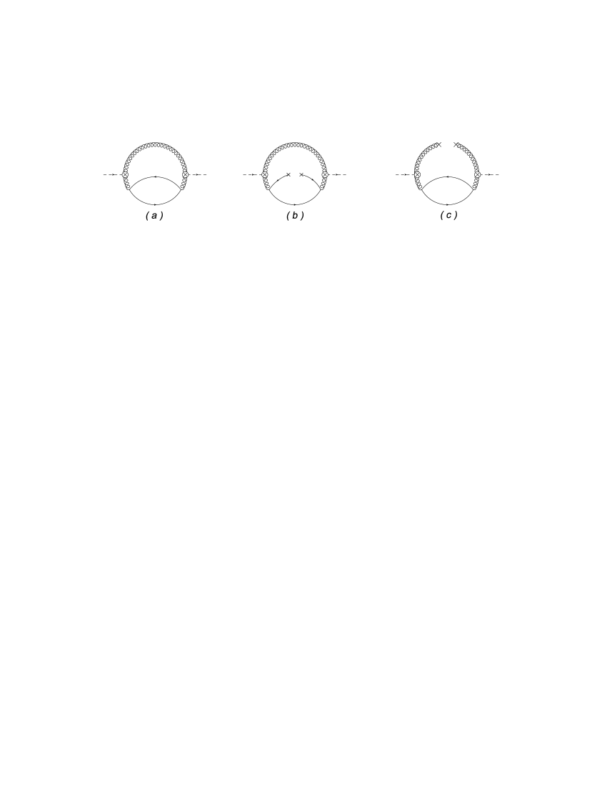
Figure 1: (a) the pertubative part; (b) the quark condensation part; (c) the gluon condensation part

With the fermion contributions containing the fermion propagators and the quark condensations, the correlation function $\Pi(q^{2})$ can be divided as:

$$\Pi(q^{2}) = \Pi^{1}(q^{2})+\Pi^{f}(q^{2})$$ (9)

where, the $\Pi^{1}(q^{2})$ is the correlation function without fermion contributions, and was given by Bagan and SteeleBagan:1990plb . The $\Pi^{f}(q^{2})$ stands for the fermion part. With OPE, we have

$$\Pi^{f}(q^{2}) = C^{f}_{0}\langle\hat{O}_{0}\rangle+C^{f}_{3}\langle\hat{O}_{3}\rangle+C^{f}_{4}\langle\hat{O}_{4}\rangle+...,$$ (10)

where, $\hat{O}_{n}$ is defined above. $C^{f}_{0}$ is the Wilson coefficient for the unit operator $\hat{O}_{0}$ in Fig 1-a, and in $\overline{\emph{MS}}$ scheme, we have:

$$C^{f}_{0}(q^{2}) = ({\alpha_{s}\over\pi})^{3}(Q^{2})^{2}(5\log{Q^{2}\over\nu^{2}}-2\log^{2}{Q^{2}\over\nu^{2}}).$$ (11)

$C^{f}_{3}$ is the Wilson coefficient for operators with quark condensate. From Fig(1-b), we have:

$$C^{f}_{3}(q^{2})\langle\hat{O}_{3}\rangle = {\alpha_{s}\over\pi}[{56\over 9}m_{q}^{3}(E_{1}(m_{q}^{2}\tau)-E_{1}(s_{0}\tau)+\log{m_{q}^{2}}(1-\rho_{0}(0)))+{8m_{q}\over\tau}(\rho_{0}(\tau s_{0})$$ (12)

$$- \rho_{0}(m_{q}^{2}\tau))+{80\over 9\tau^{3}m_{q}^{3}}(\rho_{2}(m_{q}^{2}\tau)-1)]\langle q\bar{q}\rangle+{\alpha_{s}\over\pi}[{10m_{q}\over 9}(-E_{1}(m_{q}^{2}\tau)+E_{1}(\tau s_{0})$$

$$- \log{m_{q}^{2}}(1-\rho_{0}(0)))+{2\over\tau^{2}m_{q}^{3}}(\rho_{1}(m_{q}^{2}\tau)-1)+{40\over 9m_{q}^{5}\tau^{3}}(1-\rho_{2}(m_{q}^{2}\tau))]$$

$$\times \langle g_{s}q\bar{q}G\rangle+{\alpha_{s}^{2}}[{32\over 243}(-(E_{1}(m_{q}^{2}\tau)-E_{1}(\tau s_{0}))-\log{m_{q}^{2}}(1-\rho_{0}(0)))$$

$$+ {32\over 27m_{q}^{4}\tau^{2}}(1-\rho_{1}(m_{q}^{2}\tau))+{1024\over 243m_{q}^{6}\tau^{3}}(\rho_{2}(m_{q}^{2}\tau)-1)]\langle q\bar{q}q\bar{q}\rangle,$$

where, $\rho_{k}(x)$ and $E_{1}(x)$ are defined in Eq (7), and $q$ stands for the u, d and s quarks. Later, we will show that, the contributions from the parts with quark condensates are less than 1%, so in general, can be safely ignored.

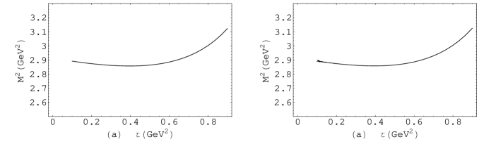
Figure 2: (a) the mass without $C^{f}_{3}$ at $s_{0}=3.8\emph{GeV}^{2}$; (b) the mass with $C^{f}_{3}$ at $s_{0}=3.8\emph{GeV}^{2}$

$C^{f}_{4}(q^{2})$ is the Wilson coefficient for the operators with gluon condensates. Generally, there are two ways to calculate the Wilson coefficientsreinders:1985pr , one is the plane wave method, by which $\Pi^{1}(q^{2})$ is given (See Eq (9)). The another is the fixed-point gauge technique, by which we have:

$$C^{f}_{4}(q^{2})\langle\hat{O}_{4}\rangle = {\alpha_{s}^{2}\over\pi}(-{13\over 3}+2\log{-q^{2}\over\nu^{2}})\langle\alpha_{s}G^{2}\rangle.$$ (13)

Substituting all the corrections ((11), (12), and (13)) back into Eq (9), we have the correlation function $\Pi(q^{2})$ and the various functions $\mathcal{R}_{k}$ with corrections from fermions. The result is shown in fig(2): We choose the reasonable platform at $\tau\in\{0.4,0.6\}$ in the region $3.6~{}\mathrm{GeV}^{2}<s_{0}<4.2~{}\mathrm{GeV}^{2}$. Within the platform, the ratio of the contribution of the unit operator term $C_{0}(q^{2})\hat{O}_{0}$, which stands for the pertubative part, to the mass determined by $\mathcal{R}_{k}$ is more than $90\%$, it enables the OPE expansion to converge sufficiently fast. Besides, in the region, the ratio of the contribution of the continuum part to the mass is less than $30\%-40\%$. It implies that this value of $s_{0}$ is appropriate for the quark-hardron duality. Within this platform we have obtained the $0^{++}$ glueball mass as: $1.721\pm 0.065~{}\mathrm{GeV}^{2}$, where the error is caused by the variable of the $s_{0}$ in the region, meanwhile, the error caused by the variable of the Borel parameter $\tau$ is very tiny so that it can be ignored. Fig (2-a) and Fig (2-b) show that, the quark condensate contributes little to the mass of the glueball, since the $C^{f}_{3}$ given in Eq (12) turns to zero at $mq\rightarrow 0$. That is why we could directly determine the mass of glueball by neglecting $C^{f}_{3}$ as long as the mass of light quarks is small.

IV Conclusion and discussion

In this paper, we analyze the contribution of the diagrams involving internal fermion lines and quark condensates. Following the traditional way, we determinate the mass of the $0^{++}$ scalar glueball as $1.728\pm 0.132~{}\mathrm{GeV}^{2}$. Comparing the result of Huang ($m\sim 1.66\mathrm{GeV}^{2}$), a little shift of the mass is resulted in by taking the fermion condensation into accout.

References

- (1) Hai-Yang. Zheng Int. J. Mod. Phys. A 24, 3392 (2009).
- (2) G. S. Bali, et al. [UKQCD Collaboration], Phys. Lett. B 309, 378 (1993);
- (3) H. Chen, J. Sexton, A. Vaccarino and D. Weingarten, Nucl. Phys. Proc. Suppl. 34, 357 (1994);
- (4) C. J. Morningstar and M. J. Peardon, Phys. Rev. D 60, 034509 (1999) ;
- (5) A. Vaccarino and D. Weingarten, Phys. Rev. D 60, 114501 (1999) [arXiv:hep-lat/9910007] ;
- (6) C. Liu, Chin. Phys. Lett. 18, 187 (2001);
- (7) D. Q. Liu, J. M. Wu and Y. Chen, High Energy Phys. Nucl. Phys. 26, 222 (2002) ;
- (8) N. Ishii, H. Suganuma and H. Matsufuru, Phys. Rev. D 66, 014507 (2002) ;
- (9) M. Loan, X. Q. Luo and Z. H. Luo, Int. J. Mod. Phys. A 21, 2905 (2006) ;
- (10) Y. Chen et al., Phys. Rev. D 73, 014516 (2006) ;
- (11) V. A. Novikov, M. A. Shifman, A. I. Vainshtein, and V. I. Zakharov Nucl. Phys. B 165, 67 (1980);
- (12) P. Pascual and R. Tarrach Phys. Lett. B 113 495 (1982);
- (13) S. Narison, Z. Phys. C, 26 209 (1984).
- (14) E. Bagan and T. G. Steele, Phys. Lett. B. 243, 413 (1990).
- (15) T. Huang, H. Jin and A. Zhang, Phys. Rev. D. 59 034026 (1999).
- (16) P. Colangelo and A. Khodjamirian [arXiv: hep-ph/0010175 ].
- (17) L. J. Reinders, H. Rubinstein and S. Yazaki Phys. Rept. 127 1 (1985).