Abstract

Inference problems with incomplete observations often aim at estimating population properties of unobserved quantities. One simple way to accomplish this estimation is to impute the unobserved quantities of interest at the individual level and then take an empirical average of the imputed values. We show that this simple imputation estimator can provide partial protection against model misspecification. We illustrate imputation estimators’ robustness to model specification on three examples: mixture model-based clustering, estimation of genotype frequencies in population genetics, and estimation of Markovian evolutionary distances. In the final example, using a representative model misspecification, we demonstrate that in non-degenerate cases, the imputation estimator dominates the plug-in estimate asymptotically. We conclude by outlining a Bayesian implementation of the imputation-based estimation.

Key words: exponential family, imputation, incomplete observations, model misspecification, robustness

1 Introduction

We are interested in robustness to model misspecification in problems with incomplete observations. Semiparametric approaches have enjoyed a lot of success in this area but these methods lack universality and so need to be fine-tuned for each problem at hand [Tsiatis, 2006, Little and An, 2004, Kang and Schafer, 2007, Chen et al., 2009]. Consequently, when practitioners are faced with nonstandard problems with incomplete observations, they are often left to their own devices. As a first step to ameliorating this deficiency, we propose a general imputation-based estimation method that provides partial protection against model misspecification for incomplete data problems.

The idea of using imputation techniques to combat model misspecification is not new. Consider the standard missing data problem of estimating population mean $\mu$ given a sample $(z_{1},y_{1}z_{1},\mathbf{x}_{1}),\dots,(z_{n},y_{n}z_{n},\mathbf{x}_{n})$, where $y_{i}$ is a response variable, $z_{i}$ is a response indicator taking value 1 if $y_{i}$ is observed and 0 otherwise, and $\mathbf{x}_{i}$ is a vector of covariates. Assuming strong ignorability, meaning that $y_{i}$ and $z_{i}$ are independent given $\mathbf{x}_{i}$, we use only those individuals for which the response variable is available to fit a response model with $m_{i}=\text{E}(y_{i}\,|\,x_{i})$ to obtain $\hat{m}_{i}$ [Rosenbaum and Rubin, 1983]. Intuitively, we can combine the empirical estimate of the mean of respondents with model-based predictions of missing $y_{i}$s for non-respondents to arrive at $\hat{\mu}=(1/n)\sum_{i:z_{i}=1}^{n}y_{i}+(1/n)\sum_{i:z_{i}=0}^{n}\hat{m}_{i}$. This estimator, called an imputation estimator by Tsiatis and Davidian [2007], will be biased if the response model is misspecified. However, the bias vanishes as the number of non-respondents decreases to zero. Using conditioning on the observed data, we can rewrite Tsiatis and Davidian [2007]’s imputation estimator as $\hat{\mu}=(1/n)\sum_{i=1}^{n}\text{E}(y_{i}\mid z_{i},y_{i}z_{i},\mathbf{x}_{i})$. In a completely unrelated missing data setting, O’Brien et al. [2009] also use expectations of complete data conditional on the observed data to arrive at novel estimators of evolutionary distances. Although O’Brien et al. [2009] used imputation by conditional expectations explicitly, these authors did not recognize the full generality of their approach.

In this paper, we investigate the behavior of imputation estimators when they are applied to general problems with incomplete observations. After formulating the generalized imputation estimator, we consider three problems with incomplete observations. We start with a mixture model and demonstrate that imputation is useful for estimating densities of mixture components. Moreover, this imputation density estimation improves accuracy of mixture model-based clustering. Next, we turn to a statistical genetics problem of estimating genotype frequencies. To keep the genetic-specific intricacies to a minimum, we construct an artificial but representative example. In spite of the introduced simplification, our results are directly applicable to a topical problem of multilocus haplotype/genotype frequency estimation, where model misspecification occurs due to a failure to account for population structure [Allen and Satten, 2008, Kraft et al., 2005]. In our last example, we consider imputation estimators of evolutionary distances between DNA sequences with partially observed continuous-time Markov chains introduced in O’Brien et al. [2009]. We fill some theoretical gaps in their work. First, we identify situations where imputation estimators are not helpful. In doing so, we - for the first time to our knowledge - use the fact that so called group-based Markov models belong to the regular exponential family [Evans and Speed, 1993]. Next, we compute almost sure limits of imputation and plug-in estimators for a particular model misspecification. Although we make several simplifying assumptions in this derivation, we believe that qualitatively our results are portable to more realistic applications considered by O’Brien et al. [2009]. We conclude by outlining a Bayesian implementation of the imputation-based estimation.

2 Generalized imputation estimators

Assume that complete data $\mathbf{x}=(\mathbf{x}_{1},\dots,\mathbf{x}_{n})$ are independent and identically distributed with each $\mathbf{x}_{i}$ distributed according to a parametric family of sampling densities $p_{T}(\mathbf{x};\boldsymbol{\theta}_{T})$ with parameters $\boldsymbol{\theta}_{T}\in\boldsymbol{\Theta}_{T}$. We observe each $\mathbf{x}_{i}$ through a transformed vector $\mathbf{y}_{i}=\mathbf{y}(\mathbf{x}_{i})$. We further assume that the true sampling density $p_{T}(\mathbf{x}_{1};\boldsymbol{\theta}_{T})$ is unknown to us and we have to erroneously postulate a misspecified model $p_{F}(\mathbf{x}_{1};\boldsymbol{\theta}_{F})$, where $\boldsymbol{\theta}_{F}\in\boldsymbol{\Theta}_{F}$ with parameter spaces $\boldsymbol{\Theta}_{T}$ and $\boldsymbol{\Theta}_{F}$ of possibly different dimensions. Despite this model misspecification, we would like to estimate $\boldsymbol{\mu}=\text{E}_{\boldsymbol{\theta}_{T}}[\mathbf{s}(\mathbf{x}_{1})]=\int\mathbf{s}(\mathbf{x}_{1})p_{T}(\mathbf{x}_{1};\boldsymbol{\theta}_{T})\text{d}\mathbf{x}_{1}$, where $\mathbf{s}$ is an arbitrary measurable function that maps complete data to an $m$-dimensional vector of summary statistics. Assuming that $\boldsymbol{\theta}_{F}$ is identifiable from incomplete data $\mathbf{y}=(\mathbf{y}_{1},\dots,\mathbf{y}_{n})$, one can simply maximize the likelihood of the observed data $\prod_{i=1}^{n}p_{F}(\mathbf{y}_{i};\boldsymbol{\theta}_{F})$ to arrive at the maximum likelihood estimate $\hat{\boldsymbol{\theta}}_{F}=\operatorname*{arg\,max}_{\boldsymbol{\theta}_{F}\in\boldsymbol{\Theta}_{F}}p_{F}(\mathbf{y};\boldsymbol{\theta}_{F})$. Then, ignoring model misspecification, we use $\hat{\boldsymbol{\theta}}_{F}$ to get the plug-in estimate of the complete-data summaries

$$\hat{\boldsymbol{\mu}}_{n}^{pi}=\text{E}_{\hat{\boldsymbol{\theta}}_{F}}[\mathbf{s}(\mathbf{x}_{1})]=\int\mathbf{s}(\mathbf{x}_{1})p_{F}(\mathbf{x}_{1};\hat{\boldsymbol{\theta}}_{F})\text{d}\mathbf{x}_{1}.$$ (1)

This estimator is destined to be biased and asymptotically inconsistent in nearly all situations due to the model misspecification.

Consider an imputation estimator

$$\hat{\boldsymbol{\mu}}_{n}^{im}=\frac{1}{n}\sum_{i=1}^{n}\text{E}_{\hat{\boldsymbol{\theta}}_{F}}\left[\mathbf{s}(\mathbf{x}_{i})\,|\,\mathbf{y}_{i}\right]=\frac{1}{n}\sum_{i=1}^{n}\int\mathbf{s}(\mathbf{x}_{i})p_{F}(\mathbf{x}_{i}\,|\,\mathbf{y}_{i};\hat{\boldsymbol{\theta}}_{F})\text{d}\mathbf{x}_{i}.$$ (2)

The motivation behind this new estimator is quite simple: in order to offer protection against model misspecification, we would like to use the empirical measure based on $\mathbf{y}_{1},\dots,\mathbf{y}_{n}$. To accomplish this, we write $\text{E}_{\boldsymbol{\theta}_{T}}\left[\mathbf{s}(\mathbf{x}_{1})\right]=\text{E}_{\boldsymbol{\theta}_{T}}\left\{\text{E}_{\boldsymbol{\theta}_{T}}\left[\mathbf{s}(\mathbf{x}_{1})\,|\,\mathbf{y}_{1}\right]\right\}\approx\mathbb{P}_{n}\text{E}_{\boldsymbol{\theta}_{T}}\left[\mathbf{s}(\mathbf{x}_{1})\,|\,\mathbf{y}_{1}\right]$ where $\mathbb{P}_{n}f=\frac{1}{n}\sum_{i=1}^{n}f(\mathbf{y}_{i})$ for any measurable function $f$. In the absence of a good alternative, we plug-in $\hat{\boldsymbol{\theta}}_{F}$ for $\boldsymbol{\theta}_{T}$ in the conditional expectations of $\mathbf{s}(\mathbf{x}_{i})$ to arrive at our imputation estimator, $\hat{\boldsymbol{\mu}}_{n}^{im}$.

If the family of distributions $\{p_{F}(\mathbf{y};\boldsymbol{\theta}_{F})\}$ satisfies usual regularity conditions we have $\hat{\boldsymbol{\theta}}_{F}\overset{\text{a.s.}}{\rightarrow}\boldsymbol{\theta}_{0}$. For example, if our model is not misspecified, i.e. $\boldsymbol{\Theta}_{F}\equiv\boldsymbol{\Theta}_{T}$, we would have $\boldsymbol{\theta}_{0}=\boldsymbol{\theta}_{T}$. Consider the family of functions $\mathcal{F}$ which consists of conditional expectations: $\mathcal{F}=\{f(\mathbf{y}_{1};\boldsymbol{\theta})=\text{E}_{\boldsymbol{\theta}}\left[\mathbf{s}(\mathbf{x}_{1})\,|\,\mathbf{y}_{1})\right],\boldsymbol{\theta}\in\boldsymbol{\Theta}_{0}\}$ for some bounded open neighborhood $\boldsymbol{\Theta}_{0}$ of the limiting value $\boldsymbol{\theta}_{0}$. If we assume that $\mathcal{F}$ has finite bracketing number $N_{[]}(\varepsilon,\mathcal{F},L_{1}(P))$ for each $\varepsilon>0$ and is pointwise continuous in $\boldsymbol{\theta}$, then one can show that $\mathbb{P}_{n}\text{E}_{\hat{\boldsymbol{\theta}}_{F}}\mathbf{s}\left[\mathbf{x}_{1})\,|\,\mathbf{y}_{1}\right]\overset{\text{a.s.}}{\rightarrow}\text{E}_{\boldsymbol{\theta}_{T}}\left\{\text{E}_{\boldsymbol{\theta}_{0}}\left[\mathbf{s}(\mathbf{x}_{1})\,|\,\mathbf{y}_{1}\right]\right\}$ using standard empirical processes machinery [van der Vaart and Wellner, 2000]. Assuming model misspecification almost inevitably leads to $\boldsymbol{\theta}_{0}\neq\boldsymbol{\theta}_{T}$. Therefore, our imputation estimator has little chance of achieving asymptotic consistency. However, if the fraction of missing information is relatively small, our new estimator can be quite close to the true value both for finite sample sizes and asymptotically.

Assume that a misspecified complete-data sampling density belongs to the regular exponential family so that $p_{F}(\mathbf{x}_{1};\boldsymbol{\theta}_{F})=a(\mathbf{x}_{1})\exp\left[\boldsymbol{\theta}_{F}^{T}\mathbf{t}(\mathbf{x}_{1})\right]/b(\boldsymbol{\theta}_{F})$, where $\mathbf{t}(\mathbf{x}_{1})=(t_{1}(\mathbf{x}_{1}),\dots,t_{r}(\mathbf{x}_{1}))$ is an $r$-dimensional vector of minimal sufficient statistics and $\boldsymbol{\theta}_{F}=(\theta_{F1},\dots,\theta_{Fr})$ is a natural parameter vector of the same dimension. Then, as noted by Sundberg [1974], the likelihood equations based on the observed data $\mathbf{y}$ can be written as $(1/n)\sum_{i=1}^{n}\text{E}_{\boldsymbol{\theta}_{F}}\left[\mathbf{t}(\mathbf{x}_{i})\,|\,\mathbf{y}_{i}\right]=\text{E}_{\boldsymbol{\theta}_{F}}\left[\mathbf{t}(\mathbf{x}_{1})\right]$. Therefore, if the complete-data summary $\mathbf{s}(\mathbf{x}_{1})$ can be expressed as a linear transformation of the sufficient statistics $\mathbf{t}(\mathbf{x}_{1})$, imposed by the falsely assumed regular exponential family model, then the plug-in estimator (1) and imputation estimator (2) coincide exactly regardless of the true sampling density of $\mathbf{x}_{1}$.

3 Mixture models and model-based clustering

Consider a mixture model with $k$ components. Let $\mathbf{h}=(h_{1},\dots,h_{n})$ be iid discrete random variables taking values in $\{1,\dots,k\}$ with probabilities $\text{Pr}\left(h_{1}=j\right)=\alpha_{j}$, $\sum_{j=1}^{k}\alpha_{j}=1$. Event $h_{i}=j$ indicates that the observed $\mathbf{y}_{i}$ is sampled from the density $p_{Fj}(\mathbf{y};\theta_{Fj})$. The complete-data sampling density becomes

$$p_{F}(h_{i},\mathbf{y}_{i};\boldsymbol{\theta}_{F})=\prod_{j=1}^{k}\left[\alpha_{j}p_{Fj}(\mathbf{y}_{i};\theta_{Fj})\right]^{1_{\{h_{i}=j\}}}$$

We obtain parameter estimates $\hat{\boldsymbol{\alpha}}=(\hat{\alpha}_{1},\dots,\hat{\alpha}_{k})$ and $\hat{\boldsymbol{\theta}}_{F}=(\hat{\theta}_{F1},\dots,\hat{\theta}_{Fk})$ by maximizing $\prod_{i=1}^{n}p_{F}(\mathbf{y}_{i};\boldsymbol{\theta}_{F})$, where $p_{F}(\mathbf{y}_{i};\boldsymbol{\theta}_{F})=\sum_{j=1}^{k}\boldsymbol{\alpha}_{j}p_{Fj}(\mathbf{y}_{i};\theta_{Fj})$. If we further assume regular exponential family sampling densities of mixture components sharing the same normalizing constant $a(\mathbf{y})$, $p_{Fj}(\mathbf{y};p_{F})=a(\mathbf{y})\exp\left[\mathbf{t}_{j}(\mathbf{y})^{T}\theta_{Fj}\right]/b_{j}(\theta_{Fj})$, then the density of the $i$th completely observed sampling unit also belongs to the regular exponential family,

$$p_{F}(h_{i},\mathbf{y}_{i};\boldsymbol{\theta}_{F})=a(\mathbf{y}_{i})\exp\left\{\sum_{j=1}^{k}1_{\{h_{i}=j\}}\mathbf{t}_{j}(\mathbf{y}_{i})^{T}\theta_{Fj}+\sum_{j=1}^{k}1_{\{h_{i}=j\}}\left[\ln\frac{\alpha_{j}}{b_{j}(\theta_{Fj})}\right]\right\}.$$

From our discussion of regular exponential family complete-data likelihoods, it is clear that plug-in and imputation estimators of mean complete-data summaries,

$$\text{E}_{\boldsymbol{\theta}_{T}}\left[1_{\{h_{i}=j\}}\mathbf{t}_{j}(\mathbf{y}_{1})\right]\text{ and }\text{E}_{\boldsymbol{\theta}_{T}}\left[1_{\{h_{i}=j\}}\right],$$ (3)

will coincide exactly regardless of the true complete-data sampling model $p_{T}(\mathbf{y}_{1},\mathbf{h}_{1};\boldsymbol{\theta}_{T})$. In fact, plug-in and imputation estimators of the second mean complete-data summary, $\text{E}_{\boldsymbol{\theta}_{T}}\left[1_{\{h_{i}=j\}}\right]$, will coincide even if densities $p_{Fj}(\mathbf{y}_{i};\boldsymbol{\theta}_{F})$ do not belong to the regular exponential family. To see this, note that the plug-in estimator in this context is $\hat{\alpha}^{pi}_{j}=\text{E}_{\hat{\alpha}_{j}}\left[1_{\{h_{i}=j\}}\right]=\text{Pr}(h_{i}=j)=\hat{\alpha}_{j}$. The estimated probability that observation $i$ belongs to component $j$ is

$$\hat{z}_{ij}=\text{E}\left(1_{\{h_{i}=j\}}\,|\,\mathbf{y}_{i}\right)=\frac{\hat{\alpha}p_{Fj}(\mathbf{y}_{i},\hat{\theta}_{Fj})}{\sum_{j=1}^{k}\hat{\alpha}p_{Fj}(\mathbf{y}_{i},\hat{\theta}_{Fj})}.$$

The imputation estimate of the $j$th mixing proportion becomes $\hat{\alpha}_{j}^{im}=(1/n)\sum_{i=1}^{n}\text{E}\left(1_{\{h_{i}=j\}}\,|\,\mathbf{y}_{i}\right)=(1/n)\sum_{i=1}^{n}\hat{z}_{ij}$. The likelihood equations for the mixture model can be rearranged to show that $\hat{\alpha}^{pi}_{j}=\hat{\alpha}^{im}_{j}$ [Redner and Walker, 1984]. Notice that estimating all of the above complete-data expectations requires unambiguously identifying mixture component $j$, which we assume is possible by imposing constraints on mixture component parameters $\theta_{F1},\dots,\theta_{Fk}$.

To make our discussion of mixture models more concrete, we simulate $n=1000$ realizations from a mixture of two log-normal distributions with the log-scale means $\mu_{1}=1.5$ and $\mu_{2}=2.5$ and standard deviations $\sigma_{1}=0.2$ and $\sigma_{2}=0.25$ respectively. The mixing proportion, $\alpha$, was set to $0.3$, completing the set of true model parameters $\boldsymbol{\theta}_{T}=(\mu_{1},\mu_{2},\sigma_{1},\sigma_{2},\alpha)$. Now, we assume a two-component normal mixture model with means $\nu_{1}$, $\nu_{2}$, possibly unequal standard deviations $\delta_{1}$, $\delta_{2}$, and a mixing proportion $\beta$. We estimate parameters $\boldsymbol{\theta}_{F}=(\nu_{1},\nu_{2},\delta_{1},\delta_{2},\beta)$ of this misspecified model using maximum likelihood via the EM algorithm [Dempster et al., 1977, Fraley and Raftery, 2003]. We show a histogram of simulated data with a normal mixture model fit in the left plot of Figure 1.

Figure 1: Mixture model example. The upper left plot shows a histogram of 1000 simulated realizations of the two-component log-normal model, described in the text. The solid line depicts the normal mixture density estimated from these simulated data. The dashed vertical lines indicate four values of threshold $c$, for which we estimate $\mu(c)=\text{E}_{\boldsymbol{\theta}_{T}}\left(1_{\{h_{1}=1\}}1_{\{y>c\}}\right)$. Results of conventional and robust estimation of these quantities are shown in the upper right plot of the figure. We repeat simulation and estimation 1000 times and plot box-plots of relative errors, $\frac{\hat{\mu}^{pi}(c)-\mu(c)}{\mu(c)}$ and $\frac{\hat{\mu}^{im}(c)-\mu(c)}{\mu(c)}$, for $c=5.0,5.5,6.0,6.5$. The bottom row shows results of mixture component density estimation and classification errors during model based clustering.

To avoid the label switching problem, we define mixture component labels by the inequality $\nu_{1}<\nu_{2}$. Equation (3) says that if we try to estimate $\text{E}_{\boldsymbol{\theta}_{T}}\left(1_{\{h_{1}=1\}}y_{1}\right)$, $\text{E}_{\boldsymbol{\theta}_{T}}\left(1_{\{h_{1}=1\}}y_{1}^{2}\right)$ or $\text{E}_{\boldsymbol{\theta}_{T}}\left(1_{\{h_{1}=1\}}\right)$, it does not matter whether we use the plug-in or imputation approach. Instead, we choose to estimate the proportion of samples from the first mixture component that fall to the right of some threshold $c$, $\mu(c)=\text{E}_{\boldsymbol{\theta}_{T}}\left(1_{\{h_{1}=1\}}1_{\{y_{1}>c\}}\right)$. The plug-in estimate of this quantity is

$$\hat{\mu}^{pi}(c)=\text{E}_{\hat{\boldsymbol{\theta}}_{F}}\left(1_{\{h_{1}=1\}}1_{\{y_{1}>c\}}\right)=\left[1-\Phi\left(\frac{c-\hat{\nu}_{1}}{\hat{\delta}_{1}}\right)\right]\hat{\beta},$$ (4)

where $\Phi$ is the standard normal cdf. Our imputation estimator becomes

$$\hat{\mu}^{im}(c)=\frac{1}{n}\sum_{i=1}^{n}\text{E}_{\hat{\boldsymbol{\theta}}_{F}}\left(1_{\{h_{i}=1\}}1_{\{y_{i}>c\}}\,|\,y_{i}\right)=\frac{1}{n}\sum_{i=1}^{n}\hat{z}_{ij}1_{\{y_{i}>z\}}.$$

Since tails of mixture components can be estimated via imputation, it should be possible to devise an imputation estimator of mixture components’ densities. Indeed, if we use a nonparametric kernel density estimator, where each observed point $i$ is weighted by $z_{ij}$, we arrive at an imputation estimate of the $j$th component density. This is potentially useful, because more accurate estimation of component densities may lead to more accurate model-based clustering [Fraley and Raftery, 2002].

The right plot of Figure 1 demonstrates results of estimating $\mu(c)$ for threshold values $c=5.0,5.5,6.0,6.5$, depicted in the left plot of the figure by the dashed vertical lines. We consider these values of $c$, because they fall into the region where sampled points can not be easily assigned to either of the two mixture components. We simulate $1000$ test data sets using already described settings. For each of the simulated data set, we compute plug-in estimates of $\mu(c)$ using the fitted correct log-normal and the misspecified normal model and the imputation under the misspecified normal model. We show box plots of the corresponding relative errors in the upper right plot of Figure 1. Although, the performance of the plug-in and imputation estimators under model misspecification is disappointingly similar, imputation density estimates, plotted in the bottom row, look more promising. We used plug-in density estimates under the correct and misspecified model and imputation density estimates to assign simulated points to two clusters. We then computed clustering classification error using R package MCLUST [Fraley and Raftery, 2003]. As shown in the lower bottom plot, clustering accuracy improves significantly under imputation estimates of mixture component densities and approaches the accuracy of clustering under the correct mixture model.

4 Estimating genotype frequencies

Here, we turn to a classical problem in statistical genetics: estimating allele and genotype frequencies from incomplete observations [Ceppelini et al., 1955]. Suppose that we measure some observable characteristic, called a phenotype, in $n$ individuals and record them in a vector $\mathbf{y}=(y_{1},\dots,y_{n})$, where each $y_{i}$ takes one of $M$ possible values in $\mathcal{C}=\{c_{1},\dots,c_{M}\}$. We further assume that each individual $i$ has an unobserved genotype $\mathbf{x}_{i}=(x_{i1},x_{i2})$, defined as an unordered pair of gene variants, called alleles, on two paired chromosomes of this individual. Suppose there are $R$ possible alleles, $\mathcal{G}=(g_{1},\dots,g_{R})$. Genotypes are assumed to determine observed phenotypes via a deterministic function $h:\mathcal{G}\times\mathcal{G}\rightarrow\mathcal{C}$ such that $h(g_{k},g_{l})=h(g_{l},g_{k})$. Making certain population genetics assumptions allows us to assume that unobserved genotypes are iid with

$$p_{T}((g_{k},g_{l});\mathbf{p},f)=\begin{cases}p_{k}^{2}(1-f)+fp_{k}&\text{ if }k=l\\ 2p_{k}p_{l}(1-f)&\text{ if }k\neq l,\end{cases}$$ (5)

where $\mathbf{p}=(p_{1},\dots,p_{R})$ are population allele frequencies and $f$ is called an inbreeding coefficient. We erroneously assume that $f=0$, reducing the model for genotype probabilities to the celebrated Hardy-Weinberg equilibrium [Hardy, 1908, Weinberg, 1908]. The falsely misspecified complete-data likelihood for datum 1 becomes

$$p_{F}(\mathbf{x}_{1};\mathbf{p})=\prod_{k>l}\left(2p_{k}p_{l}\right)^{1_{\{\mathbf{x}_{1}=(g_{k},g_{l})\}}}\prod_{k=1}^{R}(p_{i})^{2\times 1_{\{\mathbf{x}_{1}=(g_{k},g_{k})\}}}\propto\prod_{k=1}^{R}p_{k}^{t_{k}},$$

where $t_{k}=2\times 1_{\{\mathbf{x}_{1}=(g_{k},g_{k})\}}+\sum_{l=1}^{R}1_{\{\mathbf{x}_{1}=(g_{k},g_{l})\}}$. The misspecified observed-data likelihood for datum 1 is $p_{F}(y_{1};\mathbf{p})=\sum_{\mathbf{x}_{1}:h(\mathbf{x}_{1})=y_{1}}p_{F}(\mathbf{x}_{1};\mathbf{p})$.

Since the complete-data likelihood is in the regular exponential family with sufficient statistics $(t_{1},\dots,t_{R})$, the plug-in and imputation estimates of $\text{E}(\sum_{i=1}^{R}c_{i}t_{i})$ will coincide exactly. Suppose our objective is to estimate genotype frequencies $\mu_{kl}=\text{E}\left(1_{\{\mathbf{x}_{1}=(g_{k},g_{l})\}}\right)=\text{Pr}\left(\mathbf{x}_{1}=(g_{k},g_{l})\right)$. The complete-data summary $1_{\{\mathbf{x}_{1}=(g_{k},g_{l})\}}$ can not be expressed as a linear combination of the sufficient statistics, so plug-in and imputation estimation will not necessarily produce identical results. After obtaining maximum likelihood estimates of allele frequencies, $\hat{\mathbf{p}}$, the plug-in approach yields

$$\hat{\mu}_{kl}^{pi}=\hat{p}_{i}^{2}1_{\{k=l\}}+2\hat{p}_{k}\hat{p}_{l}1_{\{k\neq l\}}.$$

The imputation estimator becomes

$$\hat{\mu}_{kl}^{im}=\frac{1}{n}\sum_{i=1}^{n}\text{Pr}\left(\mathbf{x}_{i}=(g_{k},g_{l})\,|\,y_{i}=c_{j}\right)1_{\{y_{i}=c_{j}\}}=\frac{n_{j}\hat{p}_{k}^{2}}{np_{F}(c_{j};\hat{\mathbf{p}})}1_{\{k=l\}}+\frac{n_{j}2\hat{p}_{k}\hat{p}_{l}}{np_{F}(c_{j};\hat{\mathbf{p}})}1_{\{k\neq l\}},$$

where $h(g_{k},g_{l})=c_{j}$ and $n_{j}=\sum_{i=1}^{n}1_{\{y_{i}=c_{j}\}}$.

Table 1: Mappings of complete to observed data during genotype frequencies estimation. Ambiguous phenotypes are highlighted in bold.

$(g_{k},g_{l})$	$(A,A)$	$(A,B)$	$(A,C)$	$(A,D)$	$(B,B)$	$(B,C)$	$(B,D)$	$(C,C)$	$(C,D)$	$(D,D)$
$h_{1}(g_{k},g_{l})$	$aa$	$ab$	$ac$	$ad$	$bb$	$\boldsymbol{bdc}$	$\boldsymbol{bdc}$	$cc$	$cd$	$dd$
$h_{2}(g_{k},g_{l})$	$aa$	$ab$	$ac$	$ad$	$\boldsymbol{bd}$	$\boldsymbol{bdc}$	$\boldsymbol{bdc}$	$cc$	$cd$	$\boldsymbol{bd}$

Consider a particular case of the above model with four alleles: $\mathcal{G}=\{A,B,C,D\}$. Table 1 defines two mappings from genotypes to phenotypes, $h_{1}:\mathcal{G}\times\mathcal{G}\rightarrow\mathcal{C}_{1}$ and $h_{2}:\mathcal{G}\times\mathcal{G}\rightarrow\mathcal{C}_{2}$, where $\mathcal{C}_{1}=\{aa,ab,ac,ad,bb,bdc,cc,cd,dd\}$ and $\mathcal{C}_{2}=\{aa,ab,ac,ad,bd,bdc,cc,cd\}$. Notice that $\mathcal{C}_{1}$ has 9 phenotypes and $\mathcal{C}_{2}$ has 8 phenotypes. Therefore, the fraction of missing data is larger under mapping $h_{2}$ than under $h_{1}$. We simulate 1000 observed phenotypes under both mappings using complete-data model (5) with $p_{A}=0.3$, $p_{B}=0.2$, $p_{C}=0.2$, $p_{D}=0.3$ nd $f=$ 0, 0.125, 0.25, 0.375, 0.5. For each of these 10 simulated data sets, we estimate allele frequencies $\hat{p}_{A}$, $\hat{p}_{B}$, $\hat{p}_{C}$, and $\hat{p}_{D}$ using the EM algorithm and assuming that $f=0$.

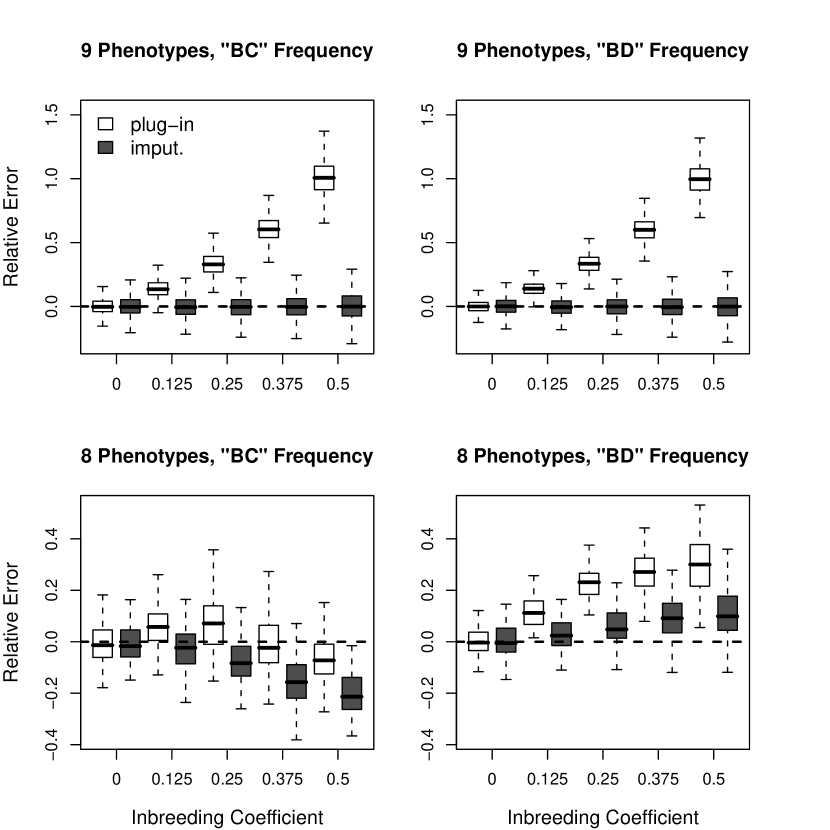
Figure 2: Genotype frequency estimation. We plot box plots of relative errors, of plug-in and imputation estimates of genotype frequencies ($\mu_{BC}$ and $\mu_{BD}$) for two incomplete data mappings, with 9 and 8 observed phenotypes. Each pair of white and grey box plots corresponds to an inbreeding coefficient that ranges from 0 to 0.5.

For phenotypes that unambiguously correspond to exactly one genotype, the empirical phenotype frequency can be used to estimate the corresponding genotype frequency. Therefore, it only makes sense to compare plug-in and imputation estimation for genotypes that correspond to ambiguously defined phenotypes. For example, under both $h_{1}$ and $h_{2}$ genotypes $(B,C)$ and $(B,D)$ correspond to the phenotype $bcd$. Suppose our goal is to estimate these genotype frequencies: $\mu_{BC}=\text{Pr}\left(\mathbf{x}_{1}=(B,C)\right)\quad\text{ and }\quad\mu_{BD}=\text{Pr}\left(\mathbf{x}_{1}=(B,D)\right)$. Plug-in estimates of these population-level quantities are

$$\hat{\mu}_{BC}^{pi}=2\hat{p}_{B}\hat{p}_{C}\quad\text{ and }\quad\hat{\mu}_{BD}^{pi}=2\hat{p}_{B}\hat{p}_{D}.$$

Imputation estimates are obtained as

$$\hat{\mu}_{BC}^{im}=\frac{n_{bcd}}{n}\frac{\hat{p}_{B}\hat{p}_{C}}{\hat{p}_{B}\hat{p}_{C}+\hat{p}_{B}\hat{p}_{D}}\quad\text{ and }\quad\hat{\mu}_{BD}^{im}=\frac{n_{bcd}}{n}\frac{\hat{p}_{B}\hat{p}_{D}}{\hat{p}_{B}\hat{p}_{C}+\hat{p}_{B}\hat{p}_{D}},$$

where $n_{bcd}=\sum_{i=1}^{n}1_{\{y_{i}=bcd\}}$ and $n=1000$. Figure 2 shows box plots of relative errors of plug-in and imputation estimators, obtained by repeating the above simulation and estimation steps 1000 times. In the case of 9 phenotypes, corresponding to $h_{1}$ mapping, the imputation estimation offers remarkable protection against model misspecification. Decreasing the number of observed phenotypes from 9 to 8 results in the imputation estimators outperforming the plug-in one only for $f=0.125$ and $f=0.25$. For the rest of inbreeding coefficient values, plug-in estimation produces better estimates of $\mu_{BC}$, while imputation estimation offers better estimates of $\mu_{BD}$. However, overall imputation relative errors are still smaller than plug-in errors.

5 Labeled evolutionary distances

Imputation estimation was proposed by O’Brien et al. [2009] in the context of estimation of evolutionary distances between molecular sequences, a standard problem in molecular evolutionary biology [Gu and Li, 1998, Yang, 2006]. Consider a $2\times n$ matrix $\mathbf{y}=\{y_{ij}\}$, where each $y_{ij}$ takes values in the $\mathcal{S}=\{1,\dots,s\}$. We assume that all columns in $\mathbf{y}$ are independently generated by the same reversible and irreducible continuous-time Markov chain (CTMC) $\{X_{t}\}$, defined on the finite state-space $\mathcal{S}$ by infinitesimal generator $\boldsymbol{\Lambda}(\boldsymbol{\theta}_{T})$. This Markov process models the evolution of DNA sequences so that the state space $\mathcal{S}$ usually consists of 4 nucleotide bases, however, a couple of alternative state-spaces are also often used. Each column $\mathbf{y}_{i}$ in $\mathbf{y}$ is produced by first drawing $y_{1i}$ from the stationary distribution of $\{X_{t}\}$, $\boldsymbol{\pi}(\boldsymbol{\theta}_{T})=(\pi_{1}(\boldsymbol{\theta}_{T}),\dots\pi_{s}(\boldsymbol{\theta}_{T}))$, running the chain for an unknown time $t$ and setting $y_{2i}=X_{t}$. For each realization $i$, we observe only the starting and ending states of the Markov chain on the time interval $[0,t]$. Here, model misspecification usually manifests itself through an incorrect parameterization of the infinitesimal generator, $\boldsymbol{\Lambda}(\boldsymbol{\theta}_{F})$. The misspecified likelihood of the observed data is $p_{F}(\mathbf{y};\boldsymbol{\theta}_{F})=\prod_{i=1}^{n}\pi_{y_{1i}}(\boldsymbol{\theta}_{T})p_{y_{1i}y_{2i}}\left(\boldsymbol{\theta}_{F},t\right)$, where $\mathbf{P}(\boldsymbol{\theta}_{F},t)=e^{\boldsymbol{\Lambda}(\boldsymbol{\theta}_{F})t}=\{p_{ij}(\boldsymbol{\theta}_{F},t)\}$ and $p_{ij}(\boldsymbol{\theta}_{F},t)=\text{Pr}\left(X_{t}=j\,|\,X_{0}=i\right)$ are finite-time transition probabilities of $\{X_{t}\}$. Notice that transition probabilities depend on $\boldsymbol{\Lambda}$ and $t$ only through their product. Therefore, we require the identifiability constraint $t=1$.

In this example, complete data consist of the full Markov chain trajectory $\mathbf{x}_{i}=\{X_{ri}:0<r<t\}$. A complete-data summary of scientific interest is $s(\mathbf{x}_{1})=N_{\mathcal{L}}$, the number of transitions of $X_{t}$ during the time interval $[0,1]$, labeled by the set of ordered state pairs $\mathcal{L}$. In the absence of complete Markov trajectories, we are interested in the mean number of labeled transitions of the stationary Markov chain, available analytically via

$$\mu=\text{E}_{\boldsymbol{\theta}_{T}}\left[s(\mathbf{x}_{1})\right]=\text{E}_{\boldsymbol{\theta}_{T}}\left(N_{\mathcal{L}}\right)=\boldsymbol{\pi}(\boldsymbol{\theta}_{T})^{T}\boldsymbol{\Lambda}_{\mathcal{L}}(\boldsymbol{\theta}_{T})\mathbf{1},$$ (6)

where $\mathbf{1}$ is an s-dimensional column vectors of 1s and $\boldsymbol{\Lambda}_{\mathcal{L}}=\{\lambda_{uv}\times 1_{\{(u,v)\in\mathcal{L}\}}\}$. In molecular evolution, this expected number of labeled Markov transitions translates into mean number of labeled mutations, allowing evolutionary biologists to measure molecular sequence similarity in a flexible manner [O’Brien et al., 2009].

The plug-in approach for estimating $\mu$ proceeds by first fitting a possibly misspecified Markov model, $\boldsymbol{\Lambda}(\boldsymbol{\theta}_{F})$ and then using the resulting parameter estimates to compute complete-data summary expectations. More specifically, we obtain $\hat{\boldsymbol{\theta}}_{F}=\operatorname*{arg\,max}_{\boldsymbol{\theta}_{F}}p(\mathbf{y};\boldsymbol{\theta}_{F})$ and obtaining plug-in and imputation estimators

$$\hat{\mu}^{pi}=\boldsymbol{\pi}(\hat{\boldsymbol{\theta}}_{F})^{T}\boldsymbol{\Lambda}(\hat{\boldsymbol{\theta}}_{F})\mathbf{1}\qquad\text{ and }\qquad\hat{\mu}^{im}=\frac{1}{n}\sum_{i=1}^{n}\text{E}_{\hat{\boldsymbol{\theta}}_{F}}\left[N^{\mathcal{L}}_{1}\,|\,X_{0}=y_{1i},X_{1}=y_{2i}\right].$$

O’Brien et al. [2009] execute two extensive simulation studies that demonstrate that the imputation estimator offers remarkable protection against misspecification of a Markovian mutational model.

5.1 Complete-data likelihood

After falsely assuming a misspecified model parameterization $\boldsymbol{\Lambda}(\boldsymbol{\theta}_{F})$ (and $\boldsymbol{\pi}(\boldsymbol{\theta}_{F})$ as a result) we condition on the initial Markov chain states and write the misspecified conditional complete-data likelihood

$$p_{F}(X_{[0,1]};\boldsymbol{\theta}_{F})\propto\left[\prod_{u\neq v}\lambda_{uv}^{n_{uv}}(\boldsymbol{\theta}_{F})\right]\times e^{\sum_{u=1}^{s}T_{u}\lambda_{uu}(\boldsymbol{\theta}_{F})},$$ (7)

where $n_{uv}$ is the number of times $X_{t}$ instantaneously jumped from $u$ to $v$ and $T_{u}$ is the total time $X_{t}$ spent in state $u$ during the time interval $[0,1]$, both summed over all $n$ realizations of the Markov chain [Guttorp, 1995]. The complete-data likelihood belongs to the curved exponential family with sufficient statistics $\mathbf{n}=\{n_{uv}\}_{u\neq v}$ and $\mathbf{T}=(T_{1},\dots,T_{s})$.

Nearly all Markov infinitesimal generators used in molecular evolutionary biology fall into the set $\mathcal{A}=\{\boldsymbol{\Lambda}=\{\lambda_{uv}\}:\lambda_{uv}=\pi_{v}\alpha_{uv}\text{ for }u\neq v\}$, where $\boldsymbol{\alpha}=\{\alpha_{uv}\}$ is a symmetric matrix. Such parameterization ensures reversibility of the Markov chain, a common assumption in the field of molecular evolution [Yang, 2006].

5.2 Group-based models

Notice that the likelihood (7) simplifies significantly if we assume a reversible model with equal diagonal entries of $\boldsymbol{\Lambda}$:

$$p_{F}(X_{[0,1]};\boldsymbol{\alpha})\propto\prod_{u<v}\alpha_{uv}^{n_{uv}+n_{vu}},$$ (8)

because $\sum_{u=1}^{s}T_{u}=1$ is the length of the observational time interval. It turns out that in molecular evolution, only so called group-based models satisfy these properties [Evans and Speed, 1993]. Group-based Markov evolutionary models can be defined as continuous-time random walks on Abelian groups. If we define an Abelian group on a Markov chain state space $\mathcal{S}$ with algebraic operation “$+$”, then entries of the corresponding group-based CTMC generator $\boldsymbol{\Lambda}$ must satisfy $\lambda_{uv}=g(u-v)$ for some function $g:\mathcal{S}\rightarrow[0,\infty)$. For example, the most general group-based model on the state space of DNA bases $\{A,G,C,T\}$ is a Kimura three-parameter model with

$$\boldsymbol{\Lambda}^{\text{K3P}}(\alpha,\beta,\gamma)=\begin{pmatrix}-&\alpha&\beta&\gamma\\ \alpha&-&\gamma&\beta\\ \beta&\gamma&-&\alpha\\ \gamma&\beta&\alpha&-\end{pmatrix},$$ (9)

corresponding to the Klein group $\mathbb{Z}_{2}\oplus\mathbb{Z}_{2}$ [Evans and Speed, 1993].

Group-based models, constructed with algebraic symmetry in mind, find extensive use in statistical phylogenetics [Sturmfels and Sullivant, 2005, Steel et al., 1998]. For us, these models are appealing because they turn the completed-data CTMC likelihood into the regular exponential family form. If we break all possible DNA mutations into three classes and define their corresponding counts $N_{AG,CT}=n_{AG}+n_{GA}+n_{CT}+n_{TC}$, $N_{AC,GT}=n_{AC}+n_{CA}+n_{GT}+n_{TG}$, and $N_{AT,GC}=n_{AT}+n_{TA}+n_{GC}+n_{CG}$, then these counts form the sufficient statistics for the Kimura three-parameter model. From our discussion of the regular exponential family it follows that plug-in and imputation estimates of $\text{E}_{\alpha,\beta,\gamma}\left(c_{1}N_{AG,CT}+c_{2}N_{AC,GT}+c_{3}N_{AT,GC}\right)$ will coincide exactly regardless of the true sampling model and of the choice of constants $c_{1}$, $c_{2}$, and $c_{3}$. This fact was not noticed by O’Brien et al. [2009], because the authors did not consider group-based models explicitly in their work.

5.3 A closer look at observed data likelihood equations

Instead of invoking properties of the regular exponential family, one can find more general conditions under which imputation and plug-in estimates of labeled evolutionary distances coincide, as demonstrated by the theorem below.

Theorem 1.

Let $\mathbf{y}=\{y_{ij}\},i=1,2,j=1,\dots,n$, be a pairwise sequence alignment generated by a CTMC with an unknown infinitesimal generator $\boldsymbol{\Lambda}(\boldsymbol{\theta}_{T})$ as described at the beginning of this section. We take $\boldsymbol{\Lambda}(\boldsymbol{\theta}_{F})$ to be a misspecified model and $\hat{\boldsymbol{\theta}}_{F}=(\hat{\theta}_{F1},\dots,\hat{\theta}_{Fr})$ to be the corresponding maximum likelihood estimator obtained from the observed data $\mathbf{y}$. If

$$\boldsymbol{\Lambda}_{\mathcal{L}}(\hat{\boldsymbol{\theta}}_{F})-\mathbf{I}\times\boldsymbol{\pi}^{T}(\hat{\boldsymbol{\theta}}_{F})\boldsymbol{\Lambda}_{\mathcal{L}}(\hat{\boldsymbol{\theta}}_{F})\mathbf{1}\in\left<\frac{\partial\boldsymbol{\Lambda}(\boldsymbol{\theta}_{F})}{\partial\theta_{F1}}\Big{|}_{\boldsymbol{\theta}_{F}=\hat{\boldsymbol{\theta}}_{F}},\dots,\frac{\partial\boldsymbol{\Lambda}(\boldsymbol{\theta}_{F})}{\partial\theta_{Fd}}\Big{|}_{\boldsymbol{\theta}_{F}=\hat{\boldsymbol{\theta}}_{F}}\right>,$$ (10)

where $\mathcal{L}\subset S^{2}\setminus\{(i,i):i\in S\}$ is a set of ordered Markov state pairs and $\boldsymbol{\Lambda}_{\mathcal{L}}=\{\lambda_{uv}\times 1_{\{(u,v)\in\mathcal{L}\}}\}$, then

$$\text{E}_{\hat{\boldsymbol{\theta}}_{F}}\left(N_{\mathcal{L}}\right)=\frac{1}{n}\sum_{i=1}^{n}\text{E}_{\hat{\boldsymbol{\theta}}_{F}}\left(N_{\mathcal{L}}\,|\,X_{0}=y_{1i},X_{1}=y_{2i}\right),$$

where $N_{\mathcal{L}}$ is the unobserved number of Markov chain transitions labeled by the set $\mathcal{L}$.

To illustrate the above theorem, consider a Kimura two-parameter model $\boldsymbol{\Lambda}^{\text{K2P}}(\alpha,\beta)=\boldsymbol{\Lambda}^{\text{K3P}}(\alpha,\beta,\beta)$, obtained by setting $\gamma=\beta$ in matrix (9) [Kimura, 1980]. For both of these models, the stationary distribution is $\boldsymbol{\pi}^{T}=(0.25,0.25,0.25,0.25)$. Let

$$\mathcal{L}_{1} =\{(A,G),(G,A),(C,T),(T,C)\}\text{ and }$$ (11)

$$\mathcal{L}_{2} =\{(A,C),(C,A),(A,T),(T,A),(C,G),(G,C),(T,G),(G,T)\}$$ (12)

be two mutational classes of interest. The partial derivatives of the Kimura two-parameter generator,

$$\frac{\partial}{\partial\alpha}\boldsymbol{\Lambda}^{\text{K2P}}(\alpha,\beta) =\frac{1}{\alpha}\left[\boldsymbol{\Lambda}_{\mathcal{L}_{1}}-\mathbf{I}\times\boldsymbol{\pi}^{t}\boldsymbol{\Lambda}_{\mathcal{L}_{1}}\mathbf{1}\right]\text{ and}$$

$$\frac{\partial}{\partial\beta}\boldsymbol{\Lambda}^{\text{K2P}}(\alpha,\beta) =\frac{1}{\beta}\left[\boldsymbol{\Lambda}_{\mathcal{L}_{1}}-\mathbf{I}\times\boldsymbol{\pi}^{t}\boldsymbol{\Lambda}_{\mathcal{L}_{2}}\mathbf{1}\right],$$

satisfy condition (10). Therefore, Theorem 1 says that plug-in and imputation estimators of $\text{E}_{\alpha,\beta}\left(N_{\mathcal{L}_{1}}\right)$ and $\text{E}_{\alpha,\beta}\left(N_{\mathcal{L}_{2}}\right)$ coincide exactly. Of course this example reiterates the fact that complete-data likelihood of the Kimura two-parameter model belongs to the regular exponential family with sufficient statistics $N_{\mathcal{L}_{1}}$ and $N_{\mathcal{L}_{2}}$.

5.4 Misspecified Kimura model: asymptotic behavior

Studying asymptotic properties of our imputation estimator is challenging in general even for the specific problem of the evolutionary distance estimation. Therefore, we turn to an elementary example to obtain some basic asymptotic results. First, we introduce the simplest group-based model on the nucleotide state space, known as a Jukes-Cantor model. The infinitesimal generator of this Markov chain is obtained by setting $\alpha=\beta$ in the Kimura two-parameter model, $\boldsymbol{\Lambda}^{\text{JC}}(\gamma)=\boldsymbol{\Lambda}^{\text{K2P}}(\gamma,\gamma)$ [Jukes and Cantor, 1969].

Theorem 2.

Assume that observed sequence data $\mathbf{y}$ was generated from the Kimura two-parameter model with generator $\boldsymbol{\Lambda}^{\text{K2P}}(\alpha,\beta)$. Let $\hat{\gamma}$ be the maximum likelihood estimate, obtained by fitting a Jukes-Cantor model with generator $\boldsymbol{\Lambda}^{\text{JC}}(\gamma)$ to $\mathbf{y}$. Then as the number of columns in $\mathbf{y}$, $n$, approaches infinity,

$$\text{E}_{\hat{\gamma}}\left(N_{\mathcal{L}_{1}}\right) \overset{\text{a.s.}}{\rightarrow}\beta-\frac{1}{4}\ln\left(\frac{1+2e^{2(\beta-\alpha)}}{3}\right)$$

$$\begin{split}\frac{1}{n}\sum_{i=1}^{n}\text{E}_{\hat{\gamma}}\left(N_{\mathcal{L}_{1}}\,|\,X_{0}=y_{1i},X_{1}=y_{2i}\right)&\overset{\text{a.s.}}{\rightarrow}\left[\beta-\frac{1}{4}\ln\left(\frac{1+2e^{2(\beta-\alpha)}}{3}\right)\right]\\ &\times\left[1+\frac{4(e^{-4\beta}+2e^{-2(\alpha+\beta)})(e^{-4\beta}-e^{-2(\alpha+\beta)})}{3(3-e^{-4\beta}-e^{-2(\alpha+\beta)})}\right],\end{split}$$

where $\mathcal{L}_{1}$ is defined by equation (11).

Figure 3: Estimator limits in the Kimura model. In both panels of the figure we plot the true value of the mean number of labeled mutations $\mu=\text{E}\left(N_{\mathcal{L}}\right)$ (solid line), the a.s. limits of the plug-in (dotted line) and imputation (dashed line) estimators.

Corollary 1.

Under the conditions of Theorem 2, define

$$\mu=\text{E}_{\alpha,\beta}\left(N_{\mathcal{L}_{1}}\right),\qquad\mu^{pi}_{\infty}=\lim_{n\rightarrow\infty}\text{E}_{\hat{\gamma}}\left(N_{\mathcal{L}_{1}}\right),\qquad\mu^{im}_{\infty}=\lim_{n\rightarrow\infty}\frac{1}{n}\sum_{i=1}^{n}\text{E}_{\hat{\gamma}}\left(N_{\mathcal{L}_{1}}\,|\,X_{0}=y_{1i},X_{1}=y_{2i}\right).$$

Then $|\mu^{im}_{\infty}-\mu|<|\mu^{pi}_{\infty}-\mu|$ when $\alpha\neq\beta$. In other words, the imputation estimator asymptotically is always better than the plug-in one.

To illustrate the above theorem and its corollary we plot the true value ($\mu$) and a.s. limits of the plug-in ($\mu^{pi}_{\infty}$) and imputation ($\mu^{im}_{\infty}$) estimators as function of $\beta$ in Figure 3. We fix $\alpha=0.01$ in the left panel and $\alpha=0.1$ in the right panel. Roughly speaking, the left panel shows the behavior of the estimators when the overall mutation rate is low, while the right panel corresponds to a high mutation rate scenario. The lower the mutation rate, the better our imputation estimator behaves asymptotically. This property of the imputation estimation is expected, because low mutation rate translates into lower fraction of missing data, which in turn makes the imputation estimation more powerful. We have already seen this behavior of the imputation estimator in the previous examples.

6 Bayesian implementation

6.1 General recipe

Although all examples so far were analyzed from the maximum likelihood perspective, one can easily perform imputation-based estimation in a Bayesian framework. To accomplish this, we first need to assign a prior distribution $p(\boldsymbol{\theta}_{F})$ to the parameters of our misspecified model $p_{F}(\mathbf{y};\boldsymbol{\theta}_{F})$. We assume that it is possible to obtain either the posterior distribution $p_{F}(\boldsymbol{\theta}_{F}\,|\,\mathbf{y})$ or the augmented posterior $p_{F}(\boldsymbol{\theta}_{F},\mathbf{x}\,|\,\mathbf{y})$, possibly approximating these distributions via Markov chain Monte Carlo (MCMC) [Tanner and Wong, 1987]. Using these posterior distributions, we define plug-in and two imputation predictive distributions

$$p\left(\text{E}_{\boldsymbol{\theta}_{F}}[\mathbf{s}(\mathbf{x}_{1})]\,\big{|}\,\mathbf{y}\right),\qquad p\left(\frac{1}{n}\sum_{i=1}^{n}\mathbf{s}(\mathbf{x}_{i})\,\Big{|}\,\mathbf{y}\right),\qquad\text{ and }\qquad p\left(\frac{1}{n}\sum_{i=1}^{n}\text{E}_{\boldsymbol{\theta}_{F}}[\mathbf{s}(\mathbf{x}_{i})\,|\,\mathbf{y}_{i}]\,\Big{|}\,\mathbf{y}\right).$$

As before, we hope that the latter two will provide us some protection against model misspecification. These last two predictive distributions have the same mean, but conditioning reduces the variance of the third distribution. This is similar to Rao-Blackwellization in Monte Carlo sampling [Casella and Robert, 1996], but since we are working under the assumption of model misspecification, smaller variance is not necessary a desirable property of a predictive distribution.

6.2 Bayesian estimation of genotype frequencies

To illustrate the Bayesian implementation of our procedure, we revisit the genotype frequency estimation example. We generate 10 phenotype samples using the two genotype-to-phenotype mappings defined in Table 1 and setting the inbreeding coefficient $f$ and true allele frequencies to the values we used in the original example. We place $\text{Dirichlet}(1,1,1,1)$ prior on allele frequencies and approximate the posterior distribution of complete data (genotype counts) and allele frequencies via Gibbs sampling.

Recall that our goal is to estimate genotype frequency $\mu_{k,l}=\text{Pr}\left(\mathbf{x}_{1}=(g_{k},g_{l})\right)$. For $(g_{k},g_{l})=(B,C)$ and $(g_{k},g_{l})=(B,D)$, we report posterior distributions of

$$2p_{k}p_{l},\qquad\frac{1}{n}\sum_{i=1}^{n}1_{\{\mathbf{x}_{i}=(g_{k},g_{l})\}}=\frac{m_{kl}}{n},\quad\text{ and }\quad\frac{1}{n}\sum_{i=1}^{n}\text{E}\left(\mathbf{x}_{i}=(g_{k},g_{l})\,|\,y_{i}\right)=\frac{n_{j}2p_{k}p_{l}}{n(2p_{B}p_{C}+2p_{B}p_{D})},$$

where $m_{kl}=\sum_{i=1}^{n}1_{\{\mathbf{x}_{i}=(g_{k},g_{l})\}}$ and $n_{j}=\sum_{i=1}^{n}1_{\{y_{i}=BCD\}}$. We report box plots of these posterior distributions in Figure 4. These box plots are not directly comparable to results in Figure 2, because our Bayesian analysis is based only on ten data sets, while the maximum analysis was done on 10,000 simulated data sets, one thousand for each value of $f$ and for each genotype-to-phenotype mapping. To make these analyses comparable, one can study frequentist properties of Bayesian plug-in and imputation estimators based, for example, on the posterior median-based estimators of allele frequencies and genotype counts. Our Bayesian results are nonetheless consistent with the maximum likelihood analysis: imputation estimators outperform the plug-in estimate in the case of nine phenotypes, none of the estimators have a uniform advantage across all values of the inbreeding coefficient in the eight phenotype case.

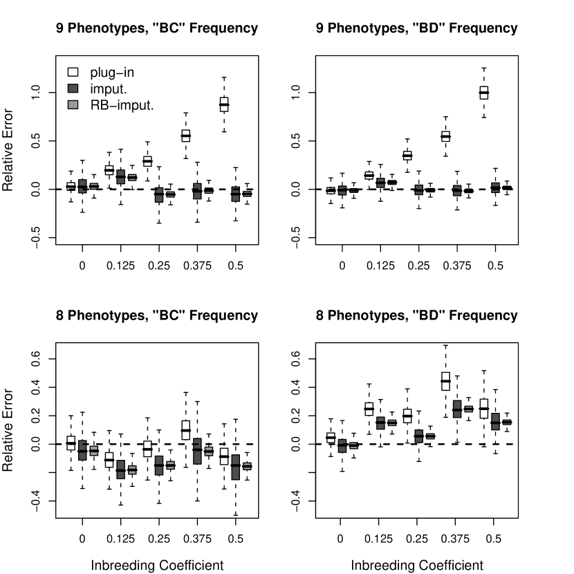
Figure 4: Genotype frequency estimation. We plot box plots of relative errors of plug-in, imputation, and Rao-Blackwellized imputation estimates of genotype frequencies ($\mu_{BC}$ and $\mu_{BD}$) for two incomplete data mappings, with 9 and 8 observed phenotypes. Each trio of white, dark grey, and light grey box plots corresponds to an inbreeding coefficient that ranges from 0 to 0.5.

We end our discussion of the Bayesian implementation of our imputation estimation by pointing out that this inferential framework is already being used in evolutionary biology, albeit somewhat informally [Zhai et al., 2007, Minin and Suchard, 2008b]. These methods extend the idea of imputation evolutionary distance estimation to multiple sequences.

7 Discussion

We generalize the notion of imputation estimators and demonstrate that such estimators can be useful in a variety of incomplete data problems under model misspecification. We use simulations as our main tool in the first two examples and provide some simple asymptotic results in our last example. So far, our experience suggests that imputation estimators perform very well under mild model misspecification and when the fraction of missing data is reasonably small. Intuitively, it is clear that imputation estimators should be more successful as the amount of missing data decreases, because in the absence of missing information these estimators turn into sample means, which are model-free and consistent estimates of appropriate population-level quantities. However, to make this intuition useful, we need to connect formally efficiency of imputation estimators with the amount of missing data and degree of model misspecification. We hope to be able to make these connections in our future work.

Studying sampling properties of imputation estimators proved to be difficult in general, especially since in practice the true sampling density of the observed data is unknown. In fact, in all our examples, we do not discuss how to compute the variance of the maximum likelihood-based imputation estimators. We recommend to use nonparametric bootstrap to explore sampling properties of imputation estimators. However, one should interpret bootstrap results with care, because imputation estimators remain biased even asymptotically. Similar care needs to be applied to the interpretation of predictive distributions in the Bayesian context.

Although we have not emphasized this throughout the paper, imputation estimators are usually easy to compute, which makes them particularly useful when a compromise between model complexity and computational efficiency results in an intentionally misspecified model. In our examples of model misspecification, we considered Gaussian mixture components, Hardy-Weinberg genotype frequencies, and parametric Markov models of DNA mutation. All these highly popular models owe a large portion of their success to their computational tractability. We argue that imputation estimators can take these and many other simple and computationally efficient models one step further outside of their usual domain of application.

Appendix

Proof of Theorem 1.

Defining $m_{kl}=\sum_{i=1}^{n}1_{\{y_{1i}=k,y_{2i}=l\}}$, the misspecified complete-data log-likelihood takes the following form:

$$l(\mathbf{y},\boldsymbol{\theta}_{F})=\sum_{k\in S}\sum_{l\in S}m_{kl}\ln p_{kl}(\boldsymbol{\theta}_{F},1),$$ (A-1)

where $p_{kl}(\boldsymbol{\theta}_{F},1)$ is the probability of $X_{1}=l$ conditional on starting $X_{0}=k$. Recall that $\mathbf{P}(\boldsymbol{\theta}_{F},1)=e^{\Lambda(\boldsymbol{\theta}_{F})}=\{p_{ij}(\boldsymbol{\theta}_{F},1)\}$. Differentiating (A-1) with respect model parameters, we arrive at the likelihood equations

$$\begin{split}\sum_{k\in E}\sum_{l\in E}\frac{m_{kl}}{p_{kl}(\boldsymbol{\theta}_{F},1)}\frac{\partial p_{kl}(\boldsymbol{\theta}_{F},1)}{\partial\theta_{Fj}}=0,j=1,\dots,r.\end{split}$$ (A-2)

From backward Kolmogorov equation $\frac{\text{d}\mathbf{P}(\boldsymbol{\theta}_{F},t)}{\text{d}t}=\Lambda(\boldsymbol{\theta}_{F})\mathbf{P}(\boldsymbol{\theta}_{F},t)$ with initial condition $\mathbf{P}(\boldsymbol{\theta}_{F},0)=\mathbf{I}$, we derive the following integral expression for the partial derivatives of transition probabilities:

$$\frac{\partial}{\partial\theta_{Fj}}\text{P}\left(\boldsymbol{\theta}_{F},1\right)=\int_{0}^{1}e^{\boldsymbol{\Lambda}(\boldsymbol{\theta}_{F})}\frac{\partial}{\partial\theta_{Fj}}\boldsymbol{\Lambda}(\boldsymbol{\theta}_{F})e^{\boldsymbol{\Lambda}(\boldsymbol{\theta}_{F})(1-\tau)}\text{d}\tau.$$

Next, we write the imputation estimator in terms of $m_{kl}$,

$$\frac{1}{n}\sum_{i=1}^{n}\text{E}_{\hat{\boldsymbol{\theta}}_{F}}\left(N_{\mathcal{L}}\,|\,X_{0}=y_{1i},X_{1}=y_{2i}\right)=\frac{1}{n}\sum_{k\in S}\sum_{l\in S}\frac{m_{kl}}{p_{kl}(\hat{\boldsymbol{\theta}}_{F},1)}\text{E}_{\hat{\boldsymbol{\theta}}_{F}}\left(N_{\mathcal{L}}1_{\{X_{1}=l\}}\,|\,X_{0}=k\right),$$

where

$$\text{E}_{\hat{\boldsymbol{\theta}}_{F}}\left(N_{\mathcal{L}}1_{\{X_{1}=l\}}\,|\,X_{0}=k\right)=\left\{\int_{0}^{1}e^{\boldsymbol{\Lambda}(\hat{\boldsymbol{\theta}}_{F})}\boldsymbol{\Lambda}_{\mathcal{L}}(\hat{\boldsymbol{\theta}}_{F})e^{\boldsymbol{\Lambda}(\hat{\boldsymbol{\theta}}_{F})(1-\tau)}\text{d}\tau\right\}_{kl}.$$ (A-3)

Derivation of the formula (A-3) can be found in [Ball and Milne, 2005] or [Minin and Suchard, 2008a]. Condition (10) says that there exist real constants $c_{1},\dots,c_{r}$ such that

$$\boldsymbol{\Lambda}_{\mathcal{L}}(\hat{\boldsymbol{\theta}}_{F})-\mathbf{I}\times\boldsymbol{\pi}^{T}(\hat{\boldsymbol{\theta}}_{F})\boldsymbol{\Lambda}_{\mathcal{L}}(\hat{\boldsymbol{\theta}}_{F})\mathbf{1}=\sum_{i=1}^{r}c_{i}\frac{\partial\boldsymbol{\Lambda}(\boldsymbol{\theta}_{F})}{\partial\theta_{Fi}}\Big{|}_{\boldsymbol{\theta}_{F}=\hat{\boldsymbol{\theta}}_{F}}.$$

Therefore, the difference between the plug-in and imputation estimators becomes

$$\begin{split}&\frac{1}{n}\sum_{i=1}^{n}\text{E}_{\hat{\boldsymbol{\theta}}_{F}}\left(N_{\mathcal{L}}\,|\,X_{0}=y_{1i},X_{1}=y_{2i}\right)-\text{E}_{\hat{\boldsymbol{\theta}}_{F}}\left(N_{\mathcal{L}}\right)=\\ &\frac{1}{n}\sum_{k\in S}\sum_{l\in S}\frac{m_{kl}}{p_{kl}(\hat{\boldsymbol{\theta}}_{F},1)}\left\{\int_{0}^{1}e^{\boldsymbol{\Lambda}(\hat{\boldsymbol{\theta}}_{F})}[\boldsymbol{\Lambda}_{\mathcal{L}}(\hat{\boldsymbol{\theta}}_{F})-\mathbf{I}\times\boldsymbol{\pi}^{T}(\hat{\boldsymbol{\theta}}_{F})\boldsymbol{\Lambda}_{\mathcal{L}}(\hat{\boldsymbol{\theta}}_{F})\mathbf{1}]e^{\boldsymbol{\Lambda}(\hat{\boldsymbol{\theta}}_{F})(1-\tau)}\text{d}\tau\right\}_{kl}=\\ &\frac{1}{n}\sum_{i=1}^{r}c_{i}\sum_{k\in S}\sum_{l\in S}\frac{m_{kl}}{p_{kl}(\hat{\boldsymbol{\theta}}_{F},1)}\left\{\int_{0}^{1}e^{\boldsymbol{\Lambda}(\hat{\boldsymbol{\theta}}_{F})}\frac{\partial\boldsymbol{\Lambda}(\boldsymbol{\theta}_{F})}{\partial\theta_{Fi}}\Big{|}_{\boldsymbol{\theta}_{F}=\hat{\boldsymbol{\theta}}_{F}}e^{\boldsymbol{\Lambda}(\hat{\boldsymbol{\theta}}_{F})(1-\tau)}\text{d}\tau\right\}_{kl}=\\ &\frac{1}{n}\sum_{i=1}^{r}c_{i}\sum_{k\in S}\sum_{l\in S}\frac{m_{kl}}{p_{kl}(\hat{\boldsymbol{\theta}}_{F},1)}\frac{\partial p_{kl}\left(\boldsymbol{\theta}_{F},1\right)}{\partial\theta_{Fi}}\Big{|}_{\boldsymbol{\theta}_{F}=\hat{\boldsymbol{\theta}}_{F}}=0,\end{split}$$

because $\hat{\boldsymbol{\theta}}_{F}$ satisfies likelihood equations (A-2). ∎

Proof of Theorem 2.

As before, let $m_{kl}=\sum_{i=1}^{n}1_{\{y_{1i}=k,y_{2i}=l\}}$. Using these site counts, define

$$m_{\mathcal{L}_{1}}=\sum_{(k,l)\in\mathcal{L}_{1}}m_{kl},\ m_{\mathcal{L}_{2}}=\sum_{(k,l)\in\mathcal{L}_{2}}m_{kl},\ m_{D}=\sum_{k=l}m_{kl},\ f_{\mathcal{L}_{1}}=\frac{m_{\mathcal{L}_{1}}}{n},\ f_{\mathcal{L}_{2}}=\frac{m_{\mathcal{L}_{2}}}{n},\ f_{D}=\frac{m_{D}}{n},$$

where $\mathcal{L}_{2}$ is defined by equation (12). Transition probabilities of the Kimura two-parameter model are obtained as

$$p_{kl}(\alpha,\beta,t)=\begin{cases}\frac{1}{4}+\frac{1}{4}e^{-4\beta t}-\frac{1}{2}e^{-2(\alpha+\beta)t}&\text{ if }(k,l)\in\mathcal{L}_{1},\\ \frac{1}{4}-\frac{1}{4}e^{-4\beta t}&\text{ if }(k,l)\in\mathcal{L}_{2},\\ \frac{1}{4}+\frac{1}{4}e^{-4\beta t}+\frac{1}{2}e^{-2(\alpha+\beta)t}&\text{ if }k=l.\end{cases}$$ (A-4)

Since the stationary distribution of the Kimura two-parameter model is uniform, $(m_{\mathcal{L}_{1}},m_{\mathcal{L}_{2}},m_{D})\sim\text{Multinomial}(p_{\mathcal{L}_{1}},p_{\mathcal{L}_{2}},p_{D})$, where

$$\begin{split}p_{\mathcal{L}_{1}}&=\sum_{(k,l)\in\mathcal{L}_{1}}\frac{1}{4}p_{kl}(\alpha,\beta,1)=\frac{1}{4}+\frac{1}{4}e^{-4\beta}-\frac{1}{2}e^{-2(\alpha+\beta)},\\ p_{\mathcal{L}_{2}}&=\sum_{(k,l)\in\mathcal{L}_{2}}\frac{1}{4}p_{kl}(\alpha,\beta,1)=\frac{1}{2}-\frac{1}{2}e^{-4\beta},\quad p_{D}=\sum_{k=l}\frac{1}{4}p_{kl}(\alpha,\beta,1)=\frac{1}{4}+\frac{1}{4}e^{-4\beta}+\frac{1}{2}e^{-2(\alpha+\beta)}.\end{split}$$

Therefore,

$$f_{\mathcal{L}_{1}}\overset{\text{a.s.}}{\rightarrow}p_{\mathcal{L}_{1}},f_{\mathcal{L}_{2}}\overset{\text{a.s.}}{\rightarrow}p_{\mathcal{L}_{2}},\text{ and }f_{D}\overset{\text{a.s.}}{\rightarrow}p_{D}$$ (A-5)

by the strong law of large numbers. We will need these a.s. limits when we express both plug-in and imputation estimators in terms of $f_{\mathcal{L}_{1}}$, $f_{\mathcal{L}_{2}}$, and $f_{D}$.

The mle of $\gamma$,$\hat{\gamma}=-\frac{1}{4}\ln\left[1-\frac{4}{3}(1-f_{D})\right]$, exists only if $1-f_{D}<3/4$. Since we know that $1-f_{D}\overset{\text{a.s.}}{\rightarrow}\frac{3}{4}-\frac{1}{4}e^{-4\beta}-\frac{1}{2}e^{-2(\alpha+\beta)}<\frac{3}{4}$, we can safely assume that $\hat{\gamma}$ is well defined for large enough $n$. The plug-in estimator

$$\text{E}_{\hat{\gamma}}(N_{\mathcal{L}_{1}})=\hat{\gamma}\overset{\text{a.s.}}{\rightarrow}\frac{1}{4}\ln\left[1-\frac{4}{3}\left(\frac{3}{4}-\frac{1}{4}e^{-4\beta}-\frac{1}{2}e^{-2(\alpha+\beta)}\right)\right]=\beta-\frac{1}{4}\ln\left(\frac{1+2e^{2(\beta-\alpha)}}{3}\right).$$

To derive the limit of the imputation estimator we start with

$$\frac{1}{n}\sum_{i=1}^{n}\text{E}_{\hat{\gamma}}\left(N_{\mathcal{L}_{1}}\,|\,X_{0}=y_{1i},X_{1}=y_{2i}\right)=\sum_{k\in S}\sum_{l\in S}\frac{f_{kl}}{p_{kl}(\hat{\gamma},1)}\text{E}_{\hat{\gamma}}\left(N_{\mathcal{L}_{1}}1_{\{X_{1}=l\}}\,|\,X_{0}=k\right).$$ (A-6)

Setting $\alpha=\beta$ in (A-4), we obtain transition probabilities for the Jukes-Cantor model:

$$p_{kl}(\gamma,t)=\left(\frac{1}{4}-\frac{1}{4}e^{-4\gamma}\right)1_{\{k\neq l\}}+\left(\frac{1}{4}+\frac{3}{4}e^{-4\gamma}\right)1_{\{k=l\}}.$$ (A-7)

To get the functional form $\text{E}_{\hat{\gamma}}\left(N_{\mathcal{L}_{1}}1_{\{X_{1}=l\}}\,|\,X_{0}=k\right)$, we first notice that $\boldsymbol{\Lambda}^{\text{JC}}$ and $\boldsymbol{\Lambda}^{\text{JC}}_{\mathcal{L}_{1}}$ commute, leading to

$$\int_{0}^{1}e^{\boldsymbol{\Lambda}^{\text{JC}}(\gamma)\tau}\boldsymbol{\Lambda}^{\text{JC}}_{\mathcal{L}_{1}}(\gamma)e^{\boldsymbol{\Lambda}^{\text{JC}(\gamma)}(1-\tau)}\text{d}\tau=\boldsymbol{\Lambda}^{\text{JC}}_{\mathcal{L}_{1}}(\gamma)e^{\boldsymbol{\Lambda}^{\text{JC}}(\gamma)}\int_{0}^{1}\text{d}\tau=\boldsymbol{\Lambda}^{\text{JC}}_{\mathcal{L}_{1}}(\gamma)e^{\boldsymbol{\Lambda}^{\text{JC}}(\gamma)}.$$

Hence,

$$\text{E}_{\hat{\gamma}}\left(N_{\mathcal{L}_{1}}1_{\{X_{1}=l\}}\,|\,X_{0}=k\right)=\hat{\gamma}\left(\frac{1}{4}+\frac{3}{4}e^{-4\hat{\gamma}}\right)1_{\{(k,l)\in\mathcal{L}_{1}\}}+\hat{\gamma}\left(\frac{1}{4}-\frac{1}{4}e^{-4\hat{\gamma}}\right)1_{\{(k,l)\notin\mathcal{L}_{1}\}}.$$ (A-8)

Plugging (A-7) and (A-8) to (A-6), we arrive at

$$\begin{split}&\frac{1}{n}\sum_{i=1}^{n}\text{E}_{\hat{\gamma}}\left(N_{\mathcal{L}_{1}}\,|\,X_{0}=y_{1i},X_{1}=y_{2i}\right)=\hat{\gamma}\left[1+4e^{-4\hat{\gamma}}\left(\frac{f_{\mathcal{L}_{1}}}{1-e^{-4\hat{\gamma}}}-\frac{f_{D}}{1+3e^{-4\hat{\gamma}}}\right)\right]\\ &=-\frac{1}{4}\ln\left[1-\frac{4}{3}(1-f_{D})\right]\times\left[1+\left(1-\frac{4}{3}(1-f_{D})\right)\left(\frac{3f_{\mathcal{L}_{1}}}{1-f_{D}}-1\right)\right].\end{split}$$

Plugging in limits (A-5) in the above formula produces the desired result. ∎

Proof of Corollary 1.

Defining $A=(e^{-4\beta}+2e^{-2(\alpha+\beta)})/3$, we write the limiting difference of the imputation and plug-in estimates as

$$\mu^{im}_{\infty}-\mu^{pi}_{\infty}=-\frac{A\ln A}{3(1-A)}e^{-4\beta}(1-e^{-2(\alpha-\beta)}).$$ (A-9)

Since $0<A\leq 1$, $\mu^{im}_{\infty}-\mu^{pi}_{\infty}$ and $\alpha-\beta$ always have the same sign. Moreover, using $e^{x}\geq 1+x$, we can show that

$$0<-\frac{A\ln A}{1-A}=\frac{\ln(1/A)}{1/A-1}<1,$$ (A-10)

when $\alpha\neq\beta$. Recall that $\mu=\boldsymbol{\pi}^{T}\boldsymbol{\Lambda}^{K2P}(\alpha,\beta)\mathbf{1}=\alpha$. leading to

$$\mu^{pi}_{\infty}-\mu=\beta-\frac{1}{4}\ln\left(\frac{1+2e^{2(\beta-\alpha)}}{3}\right)-\alpha=-\frac{1}{4}\ln\left(\frac{e^{4(\alpha-\beta)}+2e^{2(\alpha-\beta)}}{3}\right).$$

Hence, $\mu^{pi}_{\infty}-\mu$ and $\alpha-\beta$ always have opposite signs.

Case 1: $\alpha>\beta$.

We have $0<e^{-4\beta}(1-e^{-2(\alpha-\beta)})<2(\alpha-\beta)$, which together with A-10 imply $0<\mu^{im}_{\infty}-\mu^{pi}_{\infty}<\frac{2}{3}(\alpha-\beta)$. Next, we use concavity of logarithm and arrive at $\mu^{pi}_{\infty}-\mu<(\alpha-\beta)/3$. Combining these last two inequalities, we have $\mu^{im}_{\infty}-\mu<0$. Therefore,

$$\mu^{pi}_{\infty}-\mu=\mu^{pi}_{\infty}-\mu^{im}_{\infty}+\mu^{im}_{\infty}-\mu<\mu^{im}_{\infty}-\mu<0,$$

which proves the desired inequality.

Case 2: $\alpha<\beta$.

Recall that $\mu^{pi}_{\infty}>\mu$. Plugging in $0>e^{-4\beta}\left(1-e^{-2(\alpha-\beta)}\right)=e^{-2(\alpha+\beta)}\left(e^{2(\alpha-\beta)}-1\right)>e^{2(\alpha-\beta)}-1$ to (A-9) we arrive at $\frac{1}{3}\left(e^{2(\alpha-\beta)}-1\right)<\mu^{im}_{\infty}-\mu^{p}_{\infty}<0$. So

$$\mu^{im}_{\infty}-\mu=\mu^{im}_{\infty}-\mu^{pi}_{\infty}+\mu^{pi}_{\infty}-\mu>\frac{1}{3}\left(e^{2(\alpha-\beta)}-1\right)-\frac{1}{4}\ln\left(\frac{e^{4(\alpha-\beta)}+2e^{2(\alpha-\beta)}}{3}\right).$$

Defining the function on the right-hand side of the above inequality as $w(\alpha-\beta)$, we show that $w(0)=0$ and

$$w^{\prime}(\delta)=\frac{2}{3}e^{2\delta}-\frac{3\left(e^{2\delta}+1\right)}{e^{2\delta}+2}=\frac{\left(e^{2\delta}-1\right)\left(2e^{2\delta}+3\right)}{3\left(e^{2\delta}+2\right)}<0$$

for $\delta<0$. Therefore, we have $\mu^{im}_{\infty}-\mu>w(\alpha-\beta)>0$ and

$$\mu^{pi}_{\infty}-\mu=\mu^{pi}_{\infty}-\mu^{im}_{\infty}+\mu^{im}_{\infty}-\mu>\mu^{im}_{\infty}-\mu>0.$$

∎

References

- Allen and Satten [2008] A.S. Allen and G.A. Satten. Robust estimation and testing of haplotype effects in case-control studies. Genetic Epidemiology, 32:29–40, 2008.
- Ball and Milne [2005] F. Ball and R.K. Milne. Simple derivations of properties of counting processes associated with Markov renewal processes. Journal of Applied Probability, 42:1031–1043, 2005.
- Casella and Robert [1996] G. Casella and C. Robert. Rao-Blackwellisation of sampling schemes. Biometrika, 83:81–94, 1996.
- Ceppelini et al. [1955] R. Ceppelini, M. Siniscalco, and C.A.B. Smith. The estimation of gene frequencies in a random mating population. Annals of Human Genetics, 20:97–115, 1955.
- Chen et al. [2009] Y.-H. Chen, N. Chatterjee, and R.J. Carroll. Shrinkage estimators for robust and efficient inference in haplotype-based case-control studies. Journal of the American Statistical Association, 104:220–233, 2009.
- Dempster et al. [1977] A.P. Dempster, N.M. Laird, and D.B. Rubin. Maximum likelihood from incomplete data via the EM algorithm. Journal of the Royal Statistical Society, Series B, 39:1–38, 1977.
- Evans and Speed [1993] S.N. Evans and T.P. Speed. Invariants of some probability models used in phylogenetic inference. The Annals of Statistics, 21:355–377, 1993.
- Fraley and Raftery [2002] C. Fraley and A.E. Raftery. Model-based clustering, discriminant analysis, and density estimation. Journal of the American Statistical Association, 97:611–631, 2002.
- Fraley and Raftery [2003] C. Fraley and A.E. Raftery. Enhanced software for model-based clustering, density estimation, and discriminant analysis: Mclust. Journal of Classification, 20:263–286, 2003.
- Gu and Li [1998] X. Gu and W.H. Li. Estimation of evolutionary distances under stationary and nonstationary models of nucleotide substitution. Proceedings of the National Academy of Sciences, USA, 95:5899–5905, 1998.
- Guttorp [1995] P. Guttorp. Stochastic Modeling of Scientific Data. Chapman & Hall, Suffolk, Great Britain, 1995.
- Hardy [1908] G.H. Hardy. Mendelian proportions in a mixed population. Science, 28:49–50, 1908.
- Jukes and Cantor [1969] T.H Jukes and C.R. Cantor. Evolution of protein molecules, pages 21–32. Academic Press, New York, 1969.
- Kang and Schafer [2007] J.D.Y. Kang and J.L. Schafer. Demystifying double robustness: a comparison of alternative strategies for estimating a population mean from incomplete data. Statistical Science, 22:523–539, 2007.
- Kimura [1980] M. Kimura. A simple method for estimating evolutionary rates of base substitutions through comparative studies of nucleotide sequences. Journal of Molecular Evolution, 16:111–120, 1980.
- Kraft et al. [2005] P. Kraft, D.G. Cox, R.A. Paynter, D. Hunter, and I. De Vivo. Accounting for haplotype uncertainty in matched association studies: a comparison of simple and flexible techniques. Genetic Epidemiology, 28:261–272, 2005.
- Little and An [2004] R. Little and H. An. Robust likelihood-based analysis of multivariate data with missing values. Statistica Sinica, 14:949–968, 2004.
- Minin and Suchard [2008a] V.N. Minin and M.A. Suchard. Counting labeled transitions in continuous-time Markov models of evolution. Journal of Mathematical Biology, 56:391–412, 2008a.
- Minin and Suchard [2008b] V.N. Minin and M.A. Suchard. Fast, accurate and simulation-free stochastic mapping of discrete traits. Philosophical Transactions of the Royal Society B: Biological Sciences, 363:3985–3995, 2008b.
- O’Brien et al. [2009] J.D. O’Brien, V.N. Minin, and M.A. Suchard. Learning to count: Robust estimates for labeled distances between molecular sequences. Molecular Biology and Evolution, 26:801–814, 2009.
- Redner and Walker [1984] R.A. Redner and H.F. Walker. Mixture densities, maximum likelihood and the EM algorithm. SIAM Review, 26:195–239, 1984.
- Rosenbaum and Rubin [1983] P.R. Rosenbaum and D.B. Rubin. The central role of the propensity score in observational studies for causal effects. Biometrika, 70:41–55, 1983.
- Steel et al. [1998] M. Steel, M.D. Hendy, and D. Penny. Reconstructing phylogenies from nucleotide pattern probabilities: A survey and some new results. Discrete Applied Mathematics, 88:367–396, 1998.
- Sturmfels and Sullivant [2005] B. Sturmfels and S. Sullivant. Toric ideals of phylogenetic invariants. Journal of Computational Biology, 12:204–228, 2005.
- Sundberg [1974] R. Sundberg. Maximum likelihood theory for incomplete data from an exponential family. Scandinavian Journal of Statistics, 1:49–58, 1974.
- Tanner and Wong [1987] M.A. Tanner and W.H. Wong. The calculation of posterior distributions by data augmentation. Journal of the American Statistical Association, 82:528–540, 1987.
- Tsiatis and Davidian [2007] A. Tsiatis and M. Davidian. Comment: Demystifying double robustness: a comparison of alternative strategies for estimating a population mean from incomplete data. Statistical Science, 22:569–573, 2007.
- Tsiatis [2006] A.A. Tsiatis. Semiparametric Theory and Missing Data. Springer, New York, 2006.
- van der Vaart and Wellner [2000] A.W. van der Vaart and J.A. Wellner. Weak convergence and empirical processes. Springer-Verlag, New York, corrected second printing edition, 2000.
- Weinberg [1908] W. Weinberg. Über den nachweis der vererbung beim menschen. Jahreshefte des Vereins für vaterländische Naturkunde in Wüttemberg, 64:368–382, 1908.
- Yang [2006] Z. Yang. Computational Molecular Evolution. Oxford University Press, USA, 2006.
- Zhai et al. [2007] W. Zhai, M. Slatkin, and R. Nielsen. Exploring variation in the ratio among sites and lineages using mutational mappings: applications to the influenza virus. Journal of Molecular Evolution, 65:340–348, 2007.