Nanomechanical Mass Measurement using Nonlinear Response of a Graphene Membrane

Abstract

We propose a scheme to measure the mass of a single particle using the nonlinear response of a 2D nanoresonator with degenerate eigenmodes. Using numerical and analytical calculations, we show that by driving a square graphene nanoresonator into the nonlinear regime, simultaneous determination of the mass and position of an added particle is possible. Moreover, this scheme only requires measurements in a narrow frequency band near the fundamental resonance.

1 Introduction

Nanoelectromechanical (NEM) resonators hold promise as ultrasensitive mass detectors [1, 2]. NEM mass sensors (NEM-MS) rely on a resonant frequency shift $\Delta\omega$ due to an added mass $\Delta M$. However, as opposed to detecting a single adsorbed particle, to actually measure its mass $\Delta M$ from $\Delta\omega$, the position of the particle must be known. Proposed position determination schemes [3, 4, 5, 6] rely on detectors to measure the frequency shifts of several vibration modes. While this poses no problems in principle, it causes practical difficulties for NEM-MS operating in the GHz regime.

We propose a detection scheme that only requires measurements in a single narrow band centered at the fundamental mode resonance frequency of a square 2D resonator. Our method uses the nonlinear response of the resonator by exploiting the interaction between vibration modes to make information about higher modes available at the fundamental frequency. We illustrate by showing, analytically and numerically, how the nonlinear response of micrometer-size graphene resonators [8, 7] can be used for single particle mass measurements with zeptogram precision at room temperatures.

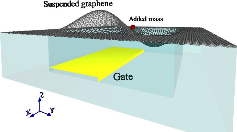
Figure 1: Possible realisation of a NEM mass spectrometer using a suspended square graphene sheet with all edges clamped. Below the graphene an electrostatic gate for actuation and transduction is placed symmetrically with respect to the X-axis and asymmetrically with respect to the Y - axis. By electrostatic actuation of vibration modes, a mass $\Delta$M located at an arbitrary position ${\bf X}_{M}=(X_{M},Y_{M})$ can be determined.

Several other technology tracks are being considered for NEM-MS devices. One is downscaling of Si-MEMS [11, 12, 13, 14, 9] where the present state-of-the-art give a minimum detectable mass of $\sim 10$ zg [9]. Another track relies on carbon nanotubes (CNTs) [15] and has already reached sub-zg levels [16, 17, 18, 10]. However, after the discovery of graphene [19], novel 2D NEMS devices have been explored [20, 21, 22, 23], including mass detectors with zg sensitivity [7]. Apart from increasing the adsorbtion cross-section, 2D-NEMS can also have degenerate flexural modes. As we show, this degeneracy makes possible to distinguish single-particle from multi-particle adsorption. Graphene also represents the ultimate material for 2D-NEMS through its combination of large strength and low mass.

2 System

We consider a square graphene sheet with mass $M$ and side length $L_{0}$ suspended in the $XY$-plane above an actuation gate (See Figure 1). The sheet is simply clamped at all edges. The gate geometry, which has a symmetry line parallel to the Y-axis, is chosen such that the fundamental and higher order modes can be excited. The transverse deflection $w({\bf X},t)$ of the membrane is given by [8]

$$\rho\ddot{w}+c\dot{w}-\sum_{\xi=X,Y}\partial_{\xi}(T_{\xi}\partial_{\xi}w)=P_{z}({\bf X},t).$$ (1)

Here $P_{z}$ is the external pressure on the sheet. This pressure comes from the electric biasing on the gate electrode. The exact geometry of the gate, and the exact ${\bf X}$-dependence of $P_{z}$ need not be known. It suffices that $P_{z}$ has the proper symmetry. And, $T_{X}=T_{Y}=T_{0}+T_{1}|\nabla w|^{2}$ are sheet tension components where $T_{0}$ is an initial tension and $T_{1}\approx 112$ N/m. Equation (1) is nonlinear due to stretching-induced tension [8]. For a particle with relative mass $\epsilon\equiv\Delta M/M$ adsorbed at ${\bf X}_{M}$, the density is $\rho({\bf X})=\rho_{0}+\Delta M\delta({\bf X}-{\bf X}_{M})$, where $\delta({\bf X})$ is the 2D delta function and $\rho_{0}$ is the density of graphene.

For future convenience, we begin by rescaling Eq.(1) into a dimensionless form. We do this by introducing the length and time scales $h_{0}=L_{0}\sqrt{T_{0}/T_{1}}$ and $t_{0}=L_{0}\sqrt{\rho_{0}/T_{0}}$, we write the deflection as $u({\bf x},\tau)=w(L_{0}{\bf x},t_{0}\tau)/h_{0}$. Equation (1) then becomes

$$[1+\epsilon\delta({\bf x}-{\bf x}_{M})]\ddot{u}+\gamma\dot{u}-\nabla^{2}u-\sum_{\xi=x,y}\partial_{\xi}(|\nabla u|^{2}\partial_{\xi}u)=p_{z}$$ (2)

where $\gamma=ct_{0}/\rho_{0}$ and $p_{z}=P_{z}t_{0}^{2}/(\rho_{0}h_{0})$.

3 Linear response

We consider first small deflections where $T_{X,Y}\approx T_{0}$, and the resonator is in the linear regime. The eigenmodes are then determined from

$$-\omega^{2}[1+\epsilon\delta({\bf x}-{\bf x}_{M})]u-\nabla^{2}u=0,\quad{\bf x}\in[0,1]^{2}.$$ (3)

Without adsorbed particles $\epsilon=0$, the first three mode shapes are $\phi_{10}=2\sin\left({\pi x}\right)\sin\left({\pi y}\right)$, $\phi_{20}=2\sin\left({2\pi x}\right)\sin\left({\pi y}\right)$, $\phi_{30}=2\sin\left({\pi x}\right)\sin\left(2{\pi y}\right)$, with eigenfrequencies $\omega_{10}^{2}=2\pi^{2}$ and $\omega_{20}^{2}=\omega_{30}^{2}=5\pi^{2}$. To linear order in $\epsilon$, adding a mass at ${\bf x}_{M}$ leads to $\omega_{1}^{2}=\omega_{10}^{2}(1-\epsilon\bar{\phi}_{1}^{2})$, $\omega_{2}^{2}=\omega_{20}^{2}(1-\epsilon{\cal N}^{2})$, and $\omega_{3}=\omega_{30}$. Here $\bar{\phi}_{m}\equiv\phi_{m0}({\bf x}_{M})$ and ${\cal N}\equiv[\bar{\phi}_{2}^{2}+\bar{\phi}_{3}^{2}]^{1/2}$. To zeroth order in $\epsilon$, $\phi_{1}=\phi_{10}$, $\phi_{2}=[\bar{\phi}_{2}\phi_{20}+\bar{\phi}_{3}\phi_{30}]/{\cal N}$ and $\phi_{3}=[{\bar{\phi}_{2}\phi_{30}-\bar{\phi}_{3}\phi_{20}}]/{\cal N}$. These solutions are illustrated in Fig. 2.

For a two-fold degenerate mode, the frequency of one mode is lowered due to particle adsorbtion. The other mode will not change frequency since it has a nodal line passing through the location $\textbf{x}_{M}$. This allows a simple test to see if more than one particle has been adsorbed. A multi-particle adsorption results in frequency shifts for both the initially degenerate modes.

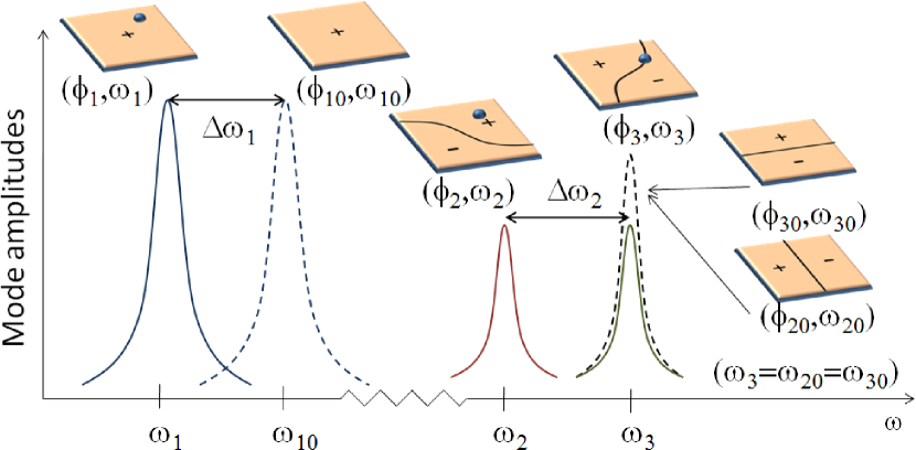
Figure 2: Amplitudes for the three lowest flexural eigenmodes as functions of drive frequency $\omega$ for weak driving. Dashed lines: Linear response without added mass. The unperturbed mode shapes $\phi_{10}$, $\phi_{20}$ and $\phi_{30}$ are indicated on the plaquettes where the locations of nodelines antinodes are shown. The modes $\phi_{20}$ and $\phi_{30}$ are degenerate. Solid lines: Linear response in the presence of an added mass. The mode functions are $\phi_{1}$, $\phi_{2}$ and $\phi_{3}$ with shapes indicated on the plaquettes. The blue dots show the position of the added mass.

4 Nonlinear response

To study the nonlinear dynamics of the system, we expand the scaled deflection $u$ in Eq.(1) in the eigenmodes $\phi_{m}({\bf x})$ of the linear problem [Eq.(3) with $\epsilon\neq 0$] as $u({\bf x},\tau)=\sum_{m=1}^{\infty}u_{m}(\tau)\phi_{m}({\bf x})$. This yields a system of coupled Duffing equations for the mode amplitudes $u_{m}$

$$D_{m}(\ddot{u}_{m}+\omega_{m}^{2}u_{m})+\gamma\dot{u}_{m}+\sum_{rst=1}^{\infty}A_{mrst}u_{r}u_{s}u_{t}=p_{m}.$$ (4)

Here $D_{m}=1+\epsilon\phi_{m}({\bf x}_{M})^{2}=1+\epsilon\tilde{\phi}_{m}^{2}$, $A_{mrst}=\int d{\bf x}\,(\nabla\phi_{m}\cdot\nabla\phi_{r})(\nabla\phi_{s}\cdot\nabla\phi_{t})$, and $p_{m}=\int d{\bf x}\,\phi_{m}p_{z}$. As $\epsilon\ll 1$ we have to lowest order in $\epsilon$, $D_{m}^{-1}\approx 1-\epsilon\tilde{\phi}_{m}^{2}\approx\omega_{m}^{2}/\omega_{m0}^{2}$.

$$(\ddot{u}_{m}+\omega_{m}^{2}u_{m})+\gamma[1-\epsilon\tilde{\phi}_{m}^{2}]\dot{u}_{m}$$

$$+\sum_{rst=1}^{\infty}A_{mrst}[1-\epsilon\tilde{\phi}_{m}^{2}]u_{r}u_{s}u_{t}=p_{m}[1-\epsilon\tilde{\phi}_{m}^{2}].$$ (5)

In what follows we will consider the weakly nonlinear regime. The cubic nonlinearities in Eq. (4) can be then be treated using the method of averaging (Krylov-Bogoliubov method). In this method, both the damping $\gamma\dot{u}$, the driving $p_{m}$, and the terms of order $u^{3}$ are of the same order and small (see for instance Ref. [28]). Formally, $\gamma$ can in this method be treated as a small parameter of a perturbation expansion. To simplify the analysis, terms of order $\cal{O}(\epsilon\gamma)$ can then be considered as higher order terms and omitted. Further, only drive frequencies close to $\omega_{10}$ and $\omega_{20}=\omega_{30}$ are used and equations for the three lowest modes suffice. These approximations give

$$\ddot{u}_{1}+\gamma\dot{u}_{1}+(\omega_{1}^{2}+5[Au_{2}^{2}+Au_{3}^{2}])u_{1}+Au_{1}^{3}=p_{1}$$

$$\ddot{u}_{2}+\gamma\dot{u}_{2}+(\omega_{2}^{2}+5[Au_{1}^{2}+Cu_{3}^{2}])u_{2}+Bu_{2}^{3}=p_{2}$$

$$\ddot{u}_{3}+\gamma\dot{u}_{3}+(\omega_{3}^{2}+5[Au_{1}^{2}+Cu_{2}^{2}])u_{3}+Bu_{3}^{3}=p_{3}$$ (6)

where $A=5\pi^{4}$, $B={161\pi^{4}}/4+{3\pi^{4}}\bar{\phi}_{2}^{2}\bar{\phi}_{3}^{2}/(2{\cal N}^{4})$ and $C\approx 41\pi^{4}/5$. The ultimate justification for the approximations leading up to Eq. (6) are the comparisons of the theoretical treatment of the system (6) with the numerical simulations of the full equations (4).

For the external force of the form $p_{z}({\bf x},\tau)=p(\tau)g({\bf x})$ where $g$ obeys the symmetry relation $g({\bf x})=g(|x-0.5|,y)$, the source terms can be written as

$$p_{1}(\tau)=D_{1}p(\tau)$$

$$p_{2}(\tau)=D_{2}p(\tau)\cos(\pi y_{M})$$

$$p_{3}(\tau)=D_{2}p(\tau)\cos(\pi x_{M}).$$

Here

$$D_{1}=2\int d{\bf x},\sin(\pi x)\sin(\pi y)g({\bf x})$$

and

$$D_{2}=2\frac{\int d{\bf x}\,\sin(\pi x)\sin(2\pi y)g({\bf x})}{\sqrt{\cos^{2}\pi x_{M}+\cos^{2}\pi y_{M}}}.$$

In the expressions for for the source terms $p_{n}$, the form of the driving force, $g({\bf x})$ is included in the coefficients $D_{1,2}$. We again stress that the exact form of $g({\bf x})$ is not important, and need not be known, as long as it has the symmetry property $g({\bf x})=g(|x-0.5|,y)$. It is this symmetry property which causes the same coeffecient $D_{2}$ to appear in both the source terms $p_{2}$ and $p_{3}$. Hence, any measurable quantity which depends only on the ratio $p_{2}/p_{1}$ will thus be a function of only the particle position ${\bf x_{M}}$. This will be used in the mass measurment scheme presented below.

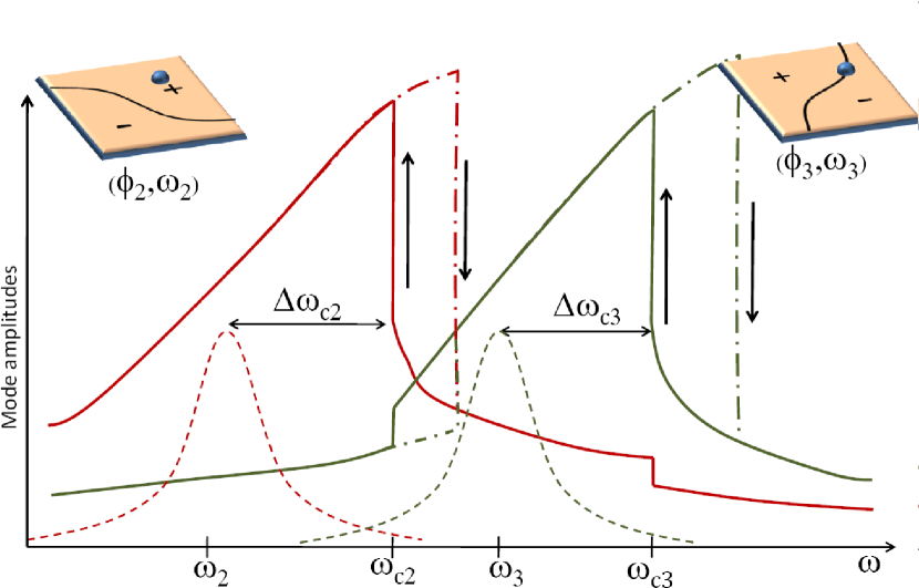
Figure 3: Amplitudes for modes 2 and 3 as functions of drive frequency $\omega$ for a square membrane with an added mass. Solid lines: Nonlinear response. Dashed lines: Linear response (see Fig. 2). By driving both modes into the nonlinear regime, the parameter $r$ [see Eq. 11] can be obtained from the frequency shifts $\Delta\omega_{c2}$ and $\Delta\omega_{c3}$. The parameter $r$ defines the nodal line of mode 3. Both $\omega_{c2}$ and $\omega_{c3}$ are measured by sweeping $\omega$ downwards. Solid curves were obtained by numerical integration of Eq. (4) with a mass fraction $\Delta M/M=0.08$% located at $(x_{M},y_{M})=(0.81,0.20)$ (quality factor $Q_{1}=3000$). Dash-dotted line: Above the frequencies $\omega_{c2,c3}$ hysteretic behavior can be observed by sweeping $\omega$ upwards.

5 Mass measurement

To determinine the position of the adsorbed mass we will use the parameters $r$ and $s$ defined as

$$r \equiv \cos(\pi y_{M})^{2}/\cos(\pi x_{M})^{2}$$ (7)

$$s \equiv 1-[\cos^{2}\left({\pi x_{M}}\right)+\cos^{2}\left({\pi y_{M}}\right)].$$ (8)

The quantity $s$ is related to the frequency shifts in the linear response regime through

$$1-s\approx\frac{1}{10}\frac{\omega_{20}^{2}-\omega_{2}^{2}}{\omega_{10}^{2}-\omega_{1}^{2}}.$$ (9)

This parameter can thus be determined by applying a weak harmonic drive of the form $p(\tau)=\cos(\omega\tau)$ and monitoring the location of resonances. Driving the system harder, still with a single frequency, puts it in the non-linear regime. However, for a single frequency excitation in the weakly non-linear regime, the coupling between the equations in (6) can be ignored and the system turns into three uncoupled Duffing equations.

$$\ddot{u}_{1}+\gamma\dot{u}_{1}+\omega_{1}^{2}u_{1}+Au_{1}^{3}=p_{1}$$

$$\ddot{u}_{2}+\gamma\dot{u}_{2}+\omega_{2}^{2}u_{2}+Bu_{2}^{3}=p_{2}$$

$$\ddot{u}_{3}+\gamma\dot{u}_{3}+\omega_{3}^{2}u_{3}+Bu_{3}^{3}=p_{3}$$ (10)

Characteristic for a driven Duffing oscillator in the nonlinear regime is the bistability region in parameter space where the system oscillates with either small or large amplitude depending on the initial conditions. This leads to the characteristic hysteresis loops seen in figure 3.

The parameter $r$ can be related to the frequency shifts by noting that the ratio of the forces $p_{2}(\tau)$ and $p_{3}(\tau)$ in Eq. (6) is given by $\sqrt{r}$. As shown in appendix, the edges of the hysteresis loops depend on the applied forces as $(\omega_{cn}^{2}-\omega_{n}^{2})^{3}\approx(9/4)^{2}Bp_{n}^{2}$ ($n$ = 2, 3) so that

$$r=\left(\frac{\omega_{c2}^{2}-\omega_{2}^{2}}{\omega_{c3}^{2}-\omega_{3}^{2}}\right)^{3}.$$ (11)

Hence, frequency measurements in the linear and nonlinear regimes can be used to determine $r$ and $s$. From $r$ and $s$ the position of the adsorbed particle can be deduced (up to symmetry of the structure). Knowing the position (in terms of $r$ and $s$) allows calculation of the mass responsivity ${\cal R}_{1}$ of the fundamental mode $\phi_{1}$ by calculating the linear frequency shift

$${\cal R}_{1}({\bf x}_{M})\approx-2{\omega_{10}}\frac{(s+r)(1+rs)}{(1+r)^{2}}$$ (12)

which gives the added mass $\Delta M=\epsilon M={\cal R}_{1}^{-1}M\Delta\omega_{1}$.

The result presented here rests on three main equations (9), (11) and (12). To obtain this result we have made two crucial assumptions relating to the symmetry of the system; the symmetry leading to mode degeneracy and the symmetry of the gate. In any real situation, these symmetries will not be exact and it is relevant to question to what extent these symmetries will need to be fulfilled. For a complete error-analysis, one must analyze the detailed reasons for lifting the degeneracies. While such a detailed analysis is beyond the scope of the present work, some observations can be readily made. Firstly, the most crucial symmetry is that of the membrane. For the scheme presented here to be relevant thus puts constraints on the intrinsic mode splitting $\Delta\omega_{23}\equiv\omega_{30}-\omega_{20}$. The first of these constraints is $\Delta\omega_{23}\ll\omega_{20}-\omega_{2}.$ When this inequality is fulfilled, the effect of an adsorbed particle on the nearly degeneraty modes is larger than the effect of imperfections leading to the intrinsic splitting. A second criterion, which is less obvious, is that

$$\Delta\omega_{23}\ll\omega_{3}-\omega_{2}$$

This criterion means that mode 3 does not shift appreciably when the particle is added.

6 Narrowband scheme

Above, we have demonstrated that frequency measurements can be used to determine the position and mass of the adsorbed particle. We now show that, by exploiting the nonlinearities in the system, this information can be obtained by measuring only in a narrow frequency band near the fundamental mode frequency $\omega_{1}$.

Equations (6) represent a system of three coupled Duffing oscillators for the modes amplitudes $u_{n}$ [$n=1,2,3$]. Here, the effective resonant frequency of a mode depends not only on the oscillation amplitude of the mode itself but also on the amplitudes of other modes so that for instance $\omega_{1}^{2}$ increase by approximately $5A\sum_{2,3}\langle u_{k}^{2}\rangle$ where $\langle\cdot\rangle$ denotes time-average over an oscillation period. This allows us to choose to use the fundamental mode to monitor the amplitudes of modes 2 and 3 as follows: In the first step, the system is excited with a single frequency signal $p(\tau)=p_{A}\cos(\omega\tau)$ and the frequency $\omega_{1}$ of the fundamental mode in the linear regime is determined. The frequency of this excitation, and detection, is henceforth kept fixed at $\omega_{1}$. A second excitation signal $p_{B}\cos(\omega\tau)$ is superimposed on the signal at frequency $\omega_{1}$. When the amplitude $p_{B}$ is low, the excitation of mode 2 in the linear regime for $\omega=\omega_{2}$ can be detected as a reduction of the oscillation amplitude of the fundamental mode. This is because the effective frequency of the fundamental mode is shifted away from $\omega_{1}$ due to the excitation of mode 2. Finally, when $p_{B}$ is increased, the mode 2 is driven into the nonlinear regime and $\omega_{c2}$ can be determined. Similarly, $\omega_{3}$ and $\omega_{c3}$ can be obtained. The effect of the mode interaction between the fundamental mode and modes 2 and 3 are shown in Fig. 4.

At first hand one may object to this scheme by noting that when the fundamental mode is strongly excited, it affects the frequencies $\omega_{2}$ and $\omega_{c2}$. However, since both $\omega_{2}^{2}$ and $\omega_{c2}^{2}$ shift by the same amount, these shifts cancel out (to first order) in the expression for $r$. The cancellation occurs also in the expression for $s$ if the resonant frequencies $\omega_{n0}$ before mass adsorption are determined through the same narrowband scheme.

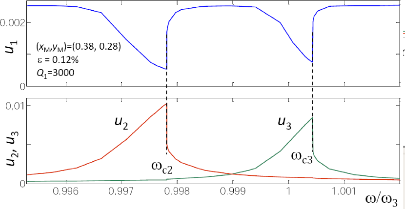
Figure 4: Mode amplitudes obtained by numerical integration of the system (4) using a gate signal $p_{A}\cos(\omega_{1}t)+p_{B}\cos(\omega t)$. Upper panel: Amplitude of mode 1 as function of variable drive frequency $\omega$. Lower panel: Amplitudes for modes 2 and 3 as functions of drive frequency $\omega$. The frequency $\omega_{1}$ is fixed at the resonance of mode 1 while $\omega$ is varied. Due to nonlinearity the modes couple. This causes the resonant frequency of mode 1 to depend on the amplitudes of modes 2 and 3. It will thus shift away from $\omega_{1}$ for finite amplitudes of modes 2 and 3. Hence, by measuring the response of mode 1, the responses of modes 2 and 3 can be probed by measuring only in a narrow frequency band around $\omega_{1}$.

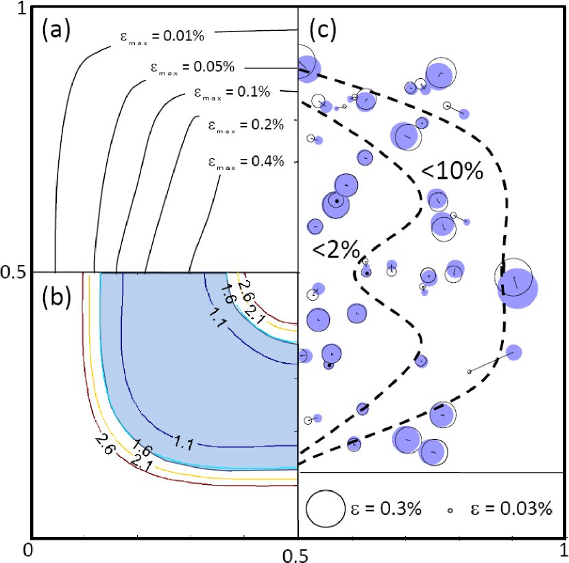
Figure 5: (a) Maximal values of $\epsilon\equiv\Delta M/M$ due to limitations of first order perturbation theory. Within each contour, mass fractions up to $\epsilon_{\rm max}$ can be determined with a 5% accuracy. (b) Contours of minimum $\epsilon Q_{1}$ where Eq. (11) is applicable. E.g., in the shaded area Eq. (11) is valid for $\epsilon>1.6/Q_{1}$. (c) Determination of randomly deposited masses using numerical integration of Eq. (4) for a membrane with $Q_{1}=3000$. The masses were uniformly distributed in the range $0.02\%<\epsilon<0.35\%$. Frequencies were determined using an accuracy of $|\Delta\omega/\omega|\approx 0.5\cdot 10^{-4}$. The positions of the deposited masses are shown by shaded symbols. The open symbols were obtained using Eqs. (9) and (11). The size of the markers are proportional to $\epsilon$. The dashed lines indicate regions where $|(\epsilon-\epsilon_{\rm exact)}/{\epsilon_{\rm exact}}|$ is less than 2% or 10%.

7 Mesurement sensitivity and range

We now consider sensitivity and range. In the NEM-MS experiments reported in the literature [11, 12, 13, 14, 9, 15, 16, 17, 18, 10], the sensitivity is usually taken as the smallest detectable mass. In our case this occurs when the particle is adsorbed at the sweet spot of the resonator at ${\bf x}_{M}=(0.5,0.5)$. This leads to $\Delta M_{\rm min}=0.5(\Delta\omega_{1}/\omega_{10})_{\rm min}M$. The intrinsic limitation on $|\Delta\omega/\omega|$ comes from thermomechanical noise that determines how small resonance shift can be reliably detected. If the detector bandwidth $\Delta\omega$ is narrower than the resonance at $\omega_{1}$ we have $|\Delta\omega/\omega|>Q_{1}^{-1}10^{-{\rm DR_{n}}/20}$ [12]. Here ${\rm DR}_{n}$ is the dynamic range of mode $n$ and $Q_{1}$ the quality factor of the fundamental mode. For modes $n=1,2,3$ we find

$${\rm DR}_{n}=10\log_{10}\left[\frac{R_{n}}{Q_{1}}\left(\frac{T_{0}}{T_{1}}\right)\frac{T_{0}L_{0}^{2}}{k_{B}T}\right],$$

where $R_{1}\approx 0.6$ and $R_{2}=R_{3}\approx 0.3$. For a device with $L_{0}=1\,\mu$m, $Q_{1}=3000$ and $\omega_{1}/(2\pi)=2$ GHz we find $\Delta M_{\rm min}\approx\frac{1}{2}MQ_{1}^{-1}10^{-2.5}\approx 0.5$ zg at $T=300$ K. At lower temperatures the sensitivity improves as $T^{1/2}$.

Thermal fluctuations also influence the determination of the frequencies $\omega_{c2,c3}$. If the system performs low-amplitude oscillations with $\omega$ close to $\omega_{c}$, thermal fluctuations can cause transitions to the high-amplitude state before $\omega_{c}$ is reached. To accurately determine $\omega_{c}$ we must have $W\ll\omega_{c}$ where $W$ is the rate for transitions to the high amplitude state. This rate obeys $W\propto e^{-RE_{T}/(k_{B}T)}$ where $E_{T}\equiv{T_{0}^{2}L_{0}^{2}}/T_{1}$ [27]. As demonstrated in Ref. [24], the strong exponential dependence of $W$ on system parameters can for NEMS lead to an enhanced sensitivity in the measurements of $\omega_{c2,c3}$ compared to the frequency measurements in the linear regimes.

We now consider the range of masses that can be reliably measured with the nonlinear mass determination scheme presented above. This must not be confused with the sensitivity discussed above which only considers the minimum detectable mass change. The range includes both upper and lower bounds on $\epsilon\equiv\Delta M/M$. The upper bound arises from omitting terms of ${\cal O}(\epsilon^{2})$ and higher in the relation $\Delta\omega_{1}={\cal R}_{1}\epsilon+{\cal O}(\epsilon^{2})$. Fig. 5a shows contours on a quadrant of the unit square corresponding to the membrane. Each contour encloses a region where the relative error due to omitting terms of ${\cal O}(\epsilon^{2})$ is less than 5%. For instance, masses with $\epsilon$ up to $\epsilon_{\rm max}=0.1\%$ can only be determined with a relative error less than 5% if they are located inside the $\epsilon_{\rm max}=0.1\%$-contour. The upper bound can be improved upon by using numerically calculated values of $\Delta\omega_{1}(\epsilon,{\bf x}_{M})$ instead of perturbation theory.

Specific to this scheme is that to determine $r$ in Eq. (11), the regions of multivalued response for modes 2 and 3 must not overlap. Not only will an overlap lead to frequency shifts (the jump in amplitude of mode 3 at $\omega=\omega_{c2}$ in Fig. 3 comes from such a shift), but we have also observed that it leads to richer dynamics, including Hopf bifurcations with limit cycles [26]. The necessary criterion for non-overlap can be shown [using Eq. (6)] to give a lower bound $\epsilon_{\rm min}\gtrsim 2.2[{\cal N}({\bf x}_{M})]^{-2}Q_{1}^{-1}$. Fig. 5b shows contours of constant values of $\epsilon_{\rm min}Q_{1}$. There, regions close to the edges and the center are excluded. Because the responsivity ${\cal R}_{1}(r,s)\rightarrow 2\omega_{10}s+{\cal O}([1-s]^{2})$ as $s\rightarrow 1$, the exclusion of the central area is superficial. For example, if we want to use the part of the membrane with $0.1<x,y<0.9$, we have approximately the lower bound $\epsilon\gtrsim 3Q^{-1}$. For a square membrane of 1 $\mu$m side ($M\approx 760$ ag), the present scheme is applicable to masses larger than $\Delta M_{\textrm{min}}\approx 0.76$ ag (assuming $Q=3000$).

8 Numerical simulations

To test the scheme we implemented an automated mass measurment algorithm which numerically integrated the system (4) with a randomly deposited mass on the membrane. The algorithm then determined the frequencies $\omega_{1,2,3}$ and $\omega_{c2,c3}$ and calculated $\epsilon$ using Eqs. (9),(11), and (12). The results are shown in Fig. 5c. The relative error in $\epsilon$ ranges from 0.1% to 98% with the larger errors near the edges where $\epsilon$ is highly sensitive to position. Masses close to the edges could be identified by overlapping responses for modes 2 and 3 in the nonlinear regimes and were discarded. As can be seen, the errors in position of the remaining particles are typically small.

9 Conclusions

In conclusion, we have proposed a scheme to determine both the position and mass of a single particle adsorbed on a vibrating graphene membrane. We have shown that by using bimodal excitation and exploiting the nonlinear response of the resonator, measurements can be restricted to a narrow frequency band near the fundamental frequency. Considering that the typical resonance frequencies of graphene membranes lie in the GHz range, this simplification offers significant experimental advantages. These measurements provide information about the resonance frequencies and the coefficients of the nonlinear terms of the dynamic equations (Kerr constants) of the high-order modes. In a resonator without special symmetries, the mass and position of the adsorbed particle can be determined using the resonance frequency shifts of three different modes —measured at a narrow frequency band near the fundamental frequency. If the resonator is square, it is possible to separate the single-particle adsorbtion events by watching out for changes of the resonance frequency of the third mode. Using a gate with a proper symmetry, it is possible to determine the mass and position of a adsorbed analyte on the membrane by using the resonance frequency shifts of modes 1 and 2 and the frequencies of the lower-edge bistability regions of modes 2 and 3.
As an example we have studied a square membrane with an area of 1 $\mu$m², eigenfrequency of 2 GHz and quality factor of $Q\approx 3000$. For this membrane the sensitivity at room temperature (minimum detectable mass change) is below 1 zeptogram with a practical operating range in the attogram region. This can be compared with, e.g., quartz crystal microbalances that have mass sensitivities in the nanogram range.

10 Appendix

We here present, for completeness, a brief derivation of the location of the bifurcation point on the so called backbone curve for the Duffing oscillator. Similar derivations can be found in most books on nonlinear systems (see for instance [28]).

Consider a harmonically driven Duffing oscillator $\ddot{x}+2\gamma\dot{x}+\omega_{0}^{2}x+\kappa x^{3}=p_{0}\cos(\omega t)$ and introduce slowly in time varying action-angle variables $r(t)$ and $\phi(t)$ such that $x=r\sin(\omega t+\phi)$ and $\dot{x}=r\omega\cos(\omega t+\phi)$. Substituting these expressions into the differential equation and averaging over the fast oscillations (see for instance [28]) gives the system

$$\dot{r}\omega = -\gamma\omega r-\frac{p_{0}}{2}\sin\phi$$

$$r\omega\dot{\phi} = \frac{\omega_{0}^{2}-\omega^{2}+(3\kappa/4)r^{2}}{2}r-\frac{p_{0}}{2}\cos\phi$$

The frequency response curve is found by solving for the stationary regime $\dot{r}=\dot{\phi}=0$. This amounts to solving the frequency response equation

$$4\gamma^{2}r^{2}\omega^{2}+r^{2}\left[(\omega_{0}^{2}-\omega^{2})+\frac{3}{4}\kappa r^{2}\right]^{2}=p_{0}^{2}.$$ (13)

We seek the solution when the bifurcation occur. This is exactly the point where $\frac{\partial\omega}{\partial r}=0$. Using this equality while taking the derivative with respect to $r$ in the frequency response equation (13), leads to an equation for the critical frequency $\omega_{c}$ (considering here the limit $\gamma\rightarrow 0$) for transition from the low to large amplitude solution

$$\left[(\omega_{0}^{2}-\omega_{c}^{2})+\frac{3}{4}\kappa r^{2}\right]+\frac{3}{2}r^{2}\kappa=0.$$

Inserting the solution for $r^{2}$ in Eq. (13) (still using $\gamma=0$) gives

$$p_{0}^{2}=\left(\frac{4}{9}\right)^{2}\frac{(\omega_{c}^{2}-\omega_{0}^{2})^{3}}{\kappa}.$$

References

- [1] K. L. Ekinci, and M. L. Roukes, Rev. Sci. Inst., 76 (2005) 061101.
- [2] A. Boisen, Nature Nanotech. 4, 404 (2009); R. G. Knobel, Nature Nanotech., 3 (2008) 525.
- [3] S. Dohn, R. Sandberg, W. Svendsen and A. Boisen. Appl. Phys. Lett., 86 (2005) 233501.
- [4] S. Dohn, W. Svendsen, A. Boisen and O. Hansen. Rev. of Sci. Inst. 78, (2007) 103303.
- [5] N. Lobontiu, I. Lupea, R. Ilic, an H. G. Craighead, J. Appl. Phys., 103 (2008) 064306.
- [6] P. S. Waggoner, and H. G. Craighead, J. Appl. Phys., 105 (2009) 054306.
- [7] C. Chen, et al., Nature Nanotech., 4 (2009) 861.
- [8] J. Atalaya, A. Isacsson, and J. M. Kinaret. Nano Lett., 8 (2008) 4196.
- [9] A. K. Naik, et al., Nature Nanotech., 4 (2009) 445.
- [10] K. Jensen, K. Kim and A. Zettl, Nature Nanotech., 3 (2008) 535 .
- [11] N. V. Lavrik, and P. G. Datskos, Appl. Phys. Lett. 82 (2003) 2697.
- [12] K. L. Ekinci, X. M. H. Huang, and M. L. Roukes, Appl. Phys. Lett., 84 (2004) 4469.
- [13] Y. T. Yang, et al., Nano. Lett., 6 (2006) 583.
- [14] X. L. Feng, R. He, P. Yang, and M. L. Roukes, Nano Lett., 7 (2007) 1953.
- [15] P. Poncharal, Z. L. Wang, D. Ugarte, and W. A. de Heer, Science, 283 (1999) 1513.
- [16] H. B. Peng, et al., Phys. Rev. Lett., 97 (2006) 087203.
- [17] B. Lassagne, D. Garcia-Sanchez, A. Aguasca and A. Bachtold, Nano Lett., 8 (2008) 3735.
- [18] H-Y. Chiu, P. Hung, H. W. Ch. Postma, and M. Bockrath, Nano.Lett., 8 (2008) 4342.
- [19] K. S. Novoselov, et al., Science, 306 (2004) 666.
- [20] J. S. Bunch et al., Science, 315 (2007) 490.
- [21] D. Garcia-Sanchez et al., Nano Lett., 8 (2008) 1399.
- [22] J. T. Robinson, et al., Nano Lett., 8 (2008) 3441.
- [23] J. S. Bunch, et al., Nano Lett., 8 (2008) 2458.
- [24] J. S. Aldridge, and A. N. Cleland, Phys. Rev. Lett., 94 (2005) 156403 .
- [25] H. W. Ch. Postma, I. Kozinsky, A. Husain, and M. L. Roukes, Appl. Phys. Lett., 86 (2005) 223105 .
- [26] J. Kozlowski, U. Parlitz and W. Lauterborn. Phys. Rev. E, 51 (1995) 1861 .
- [27] M. I. Dykman et al., Phys. Rev. E, 49 (1994) 1198 .
- [28] Ali H. Nayfeh, Dean T. Mook. Nonlinear Oscillations. Wiley-VCH 2004, p. 163-165.