Internal chaos in an open quantum system:
From Ericson to conductance fluctuations

Abstract

The model of an open Fermi-system is used for studying the interplay of intrinsic chaos and irreversible decay into open continuum channels. Two versions of the model are characterized by one-body chaos coming from disorder or by many-body chaos due to the inter-particle interactions. The continuum coupling is described by the effective non-Hermitian Hamiltonian. Our main interest is in specific correlations of cross sections for various channels in dependence on the coupling strength and degree of internal chaos. The results are generic and refer to common features of various mesoscopic objects including conductance fluctuations and resonance nuclear reactions.

1 Introduction

The problem of quantum transport is generic for all realistic quantum systems interacting with environment. A transmission of a signal through a many-body quantum aggregate of interacting particles is essentially the main instrument in studying such systems and using them for practical communication purposes. Currently this is one of the crucial lines of development of mesoscopic physics [1] with broad applications to quantum information, electronics and material science.

Historically, many ideas nowadays defining mesoscopic physics emerged in nuclear theory starting with Bohr’s concept of reactions proceeding through compound nucleus. Low-energy neutron resonances in heavy nuclei present a typical example of exceedingly complex quasistationary states in an open many-body system which serve as intermediaries in reaction processes. Later these states provided the statistical justification for the ideas of quantum chaos based on random matrix theory [2]. The detailed reviews of progressing knowledge on quantum chaos in complex atoms and nuclei can be found in [3, 4, 5, 6]; general features of mesoscopic systems of interacting fermions were stressed in [7]. The theoretical concepts of many-body quantum chaos are convincingly supported by the large-scale diagonalization of Hamiltonian matrices. Although in mesoscopic condensed matter systems one-body chaos often plays the main role, the interaction effects are also important and the analysis has many features parallel to the nuclear theory [8, 9].

When the lifetime of quasistationary states is getting small and the corresponding resonances overlap, the openness of the system becomes a decisive factor. In nuclear reactions this regime is called Ericson fluctuations [10], where certain fluctuations and correlations of cross sections are predicted. An open system can be studied by the effective non-Hermitian Hamiltonian [11, 12] that describes the intrinsic dynamics coupled to the continuum. It turns out [13] that transition from isolated to overlapping resonances implies the collectivisation of overlapped states interacting through continuum. For a small number $M$ of open channels, the restructuring of the widths leads to the segregation of $M$ short-lived states while the remaining states acquire narrow widths and long lifetime. This transition is similar to the optical super-radiance [14].

One of the brightest examples of quantum phenomena in open mesoscopic systems is given by the universal conductance fluctuations [15, 16]. There exist well pronounced similarities and some differences between them and nuclear Ericson fluctuations [17]. Some aspects of this interrelation were studied in our previous work [18]. Using the model of interacting fermions analogous to the nuclear continuum shell model [19], we analysed the behaviour of the system in function of the intrinsic interaction strength, coupling to the continuum, and number of open channels. Below we study in detail how many-body chaotic dynamics inside the system is translated into observable features of many-channel signal transmission.

2 Intrinsic chaos

Our model describes $n$ interacting fermions that occupy $m$ single-particle levels of energies $\epsilon_{s}$. The intrinsic many-body Hamiltonian can be written as

$$H_{\lambda}=H_{0}+\widetilde{\lambda}V,$$ (1)

where $H_{0}$ stands for the mean-field part describing non-interacting particles (or quasi-particles), and $V$ contains the two-body interaction between the particles with the variable strength $\tilde{\lambda}$. The matrix $H_{\lambda}$ of size $N=m!/[n!(m-n)!]$ is constructed in the many-particle basis $|k\rangle$ of the Slater determinants, $\left|k\right\rangle=a_{s_{1}}^{\dagger}\,.\,\,.\,\,.\,a_{s_{n}}^{\dagger}\left|0\right\rangle$, where $a_{s}^{\dagger}$ and $a_{s}$ are the creation and annihilation operators,

$$H_{0}=\sum_{s=1}^{m}\epsilon_{s}\,a_{s}^{\dagger}a_{s};\>\>\>\>\>\>\>\>\>\>\>\>\>\>\>\>\>\>\>V=\frac{1}{2}\sum\widetilde{V}_{s_{1}s_{2}s_{3}s_{4}}\,a_{s_{1}}^{\dagger}a_{s_{2}}^{\dagger}a_{s_{3}}a_{s_{4}}.$$ (2)

Each many-body matrix element $V_{lk}=\left<l|V|k\right>$ is a sum of a number of two-body matrix elements $\widetilde{V}_{s_{1}s_{2}s_{3}s_{4}}$ involving at most four single-particle states $|s\rangle$. For this reason, many matrix elements $V_{lk}$ vanish, and the matrix $V$ is very different from random matrices of the Gaussian orthogonal ensemble (GOE); for details, see, for example, [2, 7]. The ordered single-particle energies, $\epsilon_{s}$, are assumed to have a Poissonian distribution of spacings, with the mean level density $1/d_{\lambda}$, implying regular dynamics of the non-interacting system. The interaction $V$ belongs to an ensemble that is characterised by the variance of the normally distributed two-body random matrix elements, $\langle\widetilde{V}_{s_{1}s_{2}s_{3}s_{4}}^{2}\rangle$, and normalised in such a way that $\langle V_{l,k}^{2}\rangle=1$.

It is known [8, 9, 7] that chaotic properties of the two-body random interaction (TBRI) Hamiltonians of the type (2) are determined by the control parameter $\lambda=\widetilde{\lambda}/d_{f}$ where $d_{f}$ is the mean energy spacing between many-body states directly coupled by the two-body interaction. Note that $d_{f}\gg D_{0}$ where $D_{0}$ is the mean level spacing between many-body states. The properties of the spectra, eigenstates and observables in the model (1) have been thoroughly studied in [7]. In particular, it was shown that the critical value for the onset of strong many-body chaos is determined by the condition $\lambda>\lambda_{cr}\approx 2(m-n)/N_{f}$ where $N_{f}=n(m-n)+n(n-1)(m-n)(m-n-1)/4$.

To compare with the above model of many-body chaos, we also consider the standard random matrix model typically used to describe the onset of one-body chaos. The corresponding Hamiltonian has the form,

$$H_{\mu}=H^{\circ}+\widetilde{\mu}H_{GOE}.$$ (3)

Here $H^{\circ}$ is a diagonal matrix with the Poissonian distribution of spacings between its ordered eigenvalues, and $H_{GOE}$ is a $N\times N$ matrix belonging to the GOE. In such a description, the Hamiltonian $H_{\mu}$ can be treated as a generic model describing an electron in a quantum dot, or as a model of optical or electromagnetic waves in a closed cavity with bulk disorder. The control parameter, $\mu=\widetilde{\mu}/d_{\mu}\sqrt{N}$, determining degree of one-body chaos is the ratio of the variance of matrix elements of $H_{GOE}$ to the mean energy level spacing $d_{\mu}$ between the eigenstates of $H^{\circ}$. The transition to strong chaos occurs for $\mu>\mu_{cr}\approx 1$.

3 Coupling to continuum

Our aim is to study the statistical properties of open systems with internal dynamics described by above two Hamiltonians. According to the well developed formalism [12, 20, 21], scattering properties of an open system can be formulated with the effective non-Hermitian Hamiltonian ${\cal H}$,

$${\cal H}=H-\frac{i}{2}\,W\,;\,\,\,\,\,\,\,\,\,\,\,W_{ij}=\sum_{c=1}^{M}A_{i}^{c}A_{j}^{c},$$ (4)

where $H$ is either $H_{\lambda}$ or $H_{\mu}$. Here we neglect an additional Hermitian term (the principal value of the dispersion integral) that appears in the elimination of the continuum [22, 19]. We consider the middle of the energy spectrum, where this term vanishes. The non-Hermitian part, $W$, describes the coupling between $N$ intrinsic states $|i\rangle,|j\rangle,$ through $M$ open decay channels labelled as $a,b,c...$. The factorised structure of $W$ is dictated by the unitarity of the scattering matrix. We restrict ourselves by time-invariant systems, thus the transition amplitudes $A_{i}^{c}$ between intrinsic states $|i\rangle$ and channels $c$ are real.

The amplitudes $A_{i}^{c}$ are assumed to be random independent Gaussian variables with zero mean and variance

$$\langle A_{i}^{c}A^{c^{\prime}}_{j}\rangle=\delta_{ij}\delta_{cc^{\prime}}\,\frac{\gamma^{c}}{N}.$$ (5)

This is compatible with the GOE or TBRI models where generic intrinsic states coupled to continuum have a very complicated structure, while the decay probes specific simple components of these states related to a finite number of open channels (see discussion in [18]). Below we neglect a possible energy dependence of the amplitudes that is important near thresholds and is taken into account in realistic shell model calculations [19]. The effective parameter determining the strength of the continuum coupling can be written as

$$\kappa^{c}=\frac{\pi\gamma^{c}}{2ND},$$ (6)

and we consider $M$ equiprobable channels, $\gamma^{c}=\gamma,\,\kappa^{c}=\kappa$.

All scattering properties of the system with the non-Hermitian Hamiltonian (4) are determined by the scattering matrix, $S^{ab}=\delta_{ab}-i{\cal T}^{ab}$, with

$${\cal T}^{ab}(E)=\sum_{i,j}^{N}A_{i}^{a}\left(\frac{1}{E-{\cal H}}\right)_{ij}A_{j}^{b}.$$ (7)

The complex eigenvalues ${\cal E}$ of ${\cal H}$ coincide with the poles of the $S$-matrix and, for small $\gamma$, determine energies and widths of isolated resonances. In the critical region $\kappa\approx 1$ with crossover to overlapping resonances, the width distribution displays sharp segregation of broad short-lived (superradiant) states and very narrow long-lived (trapped) states [13, 23]. Correspondingly, the distribution of poles of the scattering matrix undergoes a transition from one to two “clouds” of poles in the complex plane of resonance energies [24]; the number of broad states coincides with the number $M$ of open channels (the rank of the matrix $W$). For the model (1), the statistical properties of resonances as a function of the interaction between particles and the coupling to continuum have been thoroughly studied in earlier papers [18, 25].

Our main interest is in the dependence of fluctuation and correlation properties of scattering on the degree of internal chaos and strength of continuum coupling. The average values of reaction cross sections, $\sigma^{ab}(E)$, are fully defined by the transition amplitudes ${\cal T}^{ab}(E)$,

$$\sigma^{ab}(E)=|{\cal T}^{ab}(E)|^{2}.$$ (8)

In our notations the cross sections are dimensionless since we omit the common factor $\pi/k^{2}$. We will use the terminology borrowed from nuclear physics referring to the $b=a$ process as “elastic” and $b\neq a$ as “inelastic” although all reactions are considered within the fixed energy window; in what follows we study both types of cross sections. We ignore the smooth potential phases irrelevant for our purposes leaving only properties due to the compound resonances and therefore to the intrinsic dynamics. According to the theory of Ericson fluctuations [10], the scattering amplitude of any process can be written as the sum of the average and fluctuating parts, ${\cal T}^{ab}(E)=\langle{\cal T}^{ab}(E)\rangle+{\cal T}^{ab}_{{\rm fl}}(E)$, with $\langle{\cal T}^{ab}_{{\rm fl}}(E)\rangle=0$. The average cross section, $\sigma=|{\cal T}|^{2}$, can be also divided into two contributions, $\langle\sigma\rangle=\langle\sigma_{{\rm dir}}\rangle+\langle\sigma_{{\rm fl}}\rangle$. Here the direct reaction cross section, $\langle\sigma_{{\rm dir}}\rangle$, is determined by the average scattering amplitude only, while $\langle\sigma_{{\rm fl}}\rangle$ is the fluctuational part also known as the compound nucleus cross section.

4 Cross section correlations

The fluctuations of both elastic and inelastic cross sections strongly depend on the coupling to the continuum. According to the standard Ericson theory, in the region of strongly overlapping resonances, $\kappa\approx 1$, the variance of both elastic and inelastic cross sections for large $M\gg 1$ can be expressed via the average cross sections, ${\rm Var}(\sigma)=\langle\sigma_{{\rm fl}}\rangle^{2}$. Our data for the many-body Hamiltonian (1) confirm this expectation for $M\geq 10$ for inelastic cross sections and any strength of interaction between particles. As for the elastic cross sections, a slight dependence on an internal chaos has been found and explained in [18].

Of special interest is the problem of correlations between different cross sections. The commonly used quantity that is discussed in nuclear and solid state physics, is the covariance $C_{{\rm fl}}$ of fluctuational cross sections,

$$C_{{\rm fl}}=\langle\sigma_{{\rm fl}}^{ab}\sigma_{{\rm fl}}^{a^{\prime}b^{\prime}}\rangle-\langle\sigma_{{\rm fl}}^{ab}\rangle\langle\sigma_{{\rm fl}}^{a^{\prime}b^{\prime}}\rangle.$$ (9)

In our case without direct processes we have $\langle\sigma\rangle=\langle\sigma_{{\rm fl}}\rangle$, therefore, below we omit the subscript “${\rm fl}$”. The analysis of the covariance $C$ shows that its value strongly depends on the type of correlations. Specifically, there are 5 types of correlations: $EE$ - elastic-elastic, when both cross sections are elastic, $EI_{1}$ and $EI_{0}$ - elastic-inelastic correlations with one and no common channels in the scattering, and $II_{1}$ and $II_{0}$ - inelastic-inelastic correlations with one and no common channels, respectively.

One should stress that the theoretical analysis of the covariance (9) encounters serious problems even for the GOE case in place of $H$ in Eq. (4) (see also Ref.[26] for different model). The second term in Eq. (9) is defined by the second moments of the scattering matrix. The corresponding expressions were obtained in Ref. [21] with the use of the super-symmetry method. In the limit $M\gg 1$, they are reduced to the Hauser-Feshbach formula, see in Ref. [2]. It is much more difficult to evaluate the first term that is determined by the four-point correlation function for matrix elements. The only analytical expressions for this term can be found in Ref. [27]. However, the result obtained there is inconsistent with our numerical data, as well as with the analysis of the universal conductance fluctuations performed in Ref. [28].

In order to understand how the cross section correlations depend on the strength of coupling to continuum and degree of internal chaos, we performed a detailed numerical study of the correlations (9) for two models (1) and (3). All data are obtained with averaging over energy $E$ at the band centre, $-0.4<E<0.4$, and over a large number of different cross sections belonging to one of the five groups defined above.

In Fig. 1 we show the correlations ($EE$) between two different elastic cross sections, $\sigma^{aa}$ and $\sigma^{bb}$ with $a\neq b$, as a function of the coupling parameter. We consider here two limiting cases, $\lambda,\mu=0.2;2.8$, for weak and strong internal chaos, respectively. A noticeable dependence on the degree of chaos is clearly seen for both models. There is an excellent agreement between $\lambda=2.8$ and $\mu=2.8$ for all values of $\kappa$. However, for weak coupling there is a small difference between the $\lambda$- and $\mu$-models. Still, the general trend of the $EE$ correlations is the same for both cases. It is interesting that the symmetry between weak and strong coupling that is known for the GOE models, and clearly seen here for strong chaos, is destroyed for weak chaos, the effect lacks an analytical explanation.

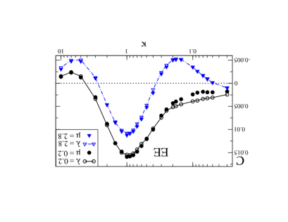
Figure 1: (colour online)Dependence of $EE$ correlations on the coupling strength, $\kappa$. Two limiting cases are shown for weak (circles) and strong (triangles) chaos. Lines and open symbols refer to the many-body model and full symbols to the one-body model, for $N=924$ and $M=4$ channels. The average was done over 1000 realisations of random matrices and the error bars (not shown) are of order of the symbol size.

Next, we consider the correlations $EI_{0}$ between different elastic-inelastic fluctuating cross sections with no common channel index, and the $II_{0}$ correlations between two different inelastic-inelastic cross sections. These are shown in Fig. 2 for the same limiting cases as above, $\lambda,\mu=0.2;2.8$. The $EI_{0}$ and $II_{0}$ correlations have a difference by a factor close to $2$ in amplitude but follow a similar trend for all three cases of internal chaos. Comparing the results for the two models we arrive at a similar result as before: an excellent agreement between $\lambda=2.8$ and $\mu=2.8$, and small deviations between the cases $\lambda\leq 1$ and $\mu\leq 1$ for weak coupling. This is more evident for the $EI_{0}$ than for the $II_{0}$ correlations.

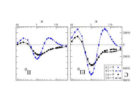
Figure 2: (colour online) Dependence of the $EI_{0}$ and $II_{0}$ correlations on $\kappa$ for the parameters of Fig. 1.

The analogous case, when there is one common channel index between the fluctuating cross sections involved in the correlation function, is shown in Fig. 3. Here the $EI_{1}$ and $II_{1}$ correlations differ by a factor close to $5$ in amplitude but behave similarly for both limiting cases of internal chaos, $\lambda,\mu=0.2$ and $2.8$. Furthermore, $EI_{1}$ correlations are independent of the degree of internal chaos whereas $II_{1}$ correlations become slightly smaller at stronger chaos. For the $EI_{1}$ correlations the correspondence between the two models is excellent for all values of $\kappa$.

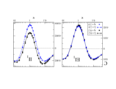
Figure 3: (colour online) Dependence of the $EI_{1}$ and $II_{1}$ correlations on $\kappa$ for the parameters of Fig. 1.

We have to stress that the correlations for strong chaos with $\lambda,\mu=2.8$, are in a good agreement if the Hermitian part of the Hamiltonian (4) is taken from the GOE.

From our data one can see that the strongest correlations occur at perfect coupling to continuum, $\kappa\approx 1$. Another remarkable property is that the correlations are either negative or positive depending on whether there is a common channel in the correlating cross sections or such channels are absent. Indeed, both $EI_{1}$ and $II_{1}$ correlations are negative around $\kappa=1$, whereas the $EI_{0}$ and $II_{0}$ correlations are positive.

For a large number of channels, $M\gg 1$, these correlations are very weak, and they are ignored in the standard Ericson theory. However, they turn out to be very important when considering the properties of conductance fluctuations, see below. Also, in nuclear physics there are situations when the number of open channels is relatively small, and one can expect that the effect of different signs of correlations can be observed experimentally. One of the new applications of such experiments can be the calibration of internal chaos with the use of scattering data.

Therefore, it is important to know the dependence of the correlations (9) on the number of channels. Our analysis has revealed that the value of the covariance $C$ is inversely proportional to the number ${\cal N}$ of terms in each group specified by the type of correlations, over which the averaging is performed in Eq. (9), see Table. Our extensive numerical data has confirmed this dependence, $C=X/{\cal N}$ with some constants $X$ that we extracted by fitting the data with the above dependence. This rule works perfectly starting from $M=2$ or $3$.

Number of Terms, ${\cal N}$
Elastic-Elastic ($EE$)	$M^{2}-M$
Elastic-Inelastic ($EI_{0}$)	$2(M^{3}-3M^{2}+2M)$
Elastic-Inelastic ($EI_{1}$)	$4(M^{2}-M)$
Inelastic-Inelastic ($II_{0}$)	$M^{4}-6M^{3}+11M^{2}-6M$
Inelastic-Inelastic ($II_{1}$)	$4(M^{3}-3M^{2}+2M)$

5 Conductance fluctuations

One of the most intriguing effects of mesoscopic physics is the universality of conductance fluctuations. In order to study this effect in the framework of our models (1) and (3), one should treat $M/2$ $b$-channels as left channels corresponding to incoming electron waves, and other $M/2$ $a$-channels, as right channels for outgoing waves. Then, we define the Landauer conductance $G$ in the standard way [15] omitting the common factor of $2e^{2}/h$),

$$G=\sum_{b=1}^{M/2}\sum_{a>M/2}^{M}\sigma^{ab}.$$ (10)

The properties of the conductance are entirely determined by the inelastic cross-sections, $b\neq a$, and for equivalent channels the average conductance (10) reads,

$$\langle G\rangle=\frac{M^{2}}{4}\langle\sigma^{ab}\rangle=\frac{M^{2}}{4}\frac{T}{F+M-1}\rightarrow\frac{MT}{4}.$$ (11)

Here $T=4\kappa/(1+\kappa)^{2}$ is the transmission coefficient, and $F=\langle\sigma_{{\rm fl}}^{aa}\rangle/\langle\sigma_{{\rm fl}}^{ab}\rangle$ is the elastic enhancement factor [29]. Our data show that the value of $F$ changes from $F=2$ to $F\approx 3$ when decreasing the strength of chaos from $\lambda,\mu=\infty$ to $\lambda,\mu=0$. The last expression in Eq. (11) is written for $M\gg 1$. As one can see, the influence of internal chaos is due to the enhancement factor $F$ only. Since there is no theory relating the enhancement factor to the degree of chaos, we used this factor as the fitting parameter. Our data manifest an excellent agreement with the expression (11) for various values of parameters $\lambda$ and $\mu$, as well as $M$. Note that for a very large number of channels the influence of internal dynamics on fluctuations disappears.

As for the variance ${\rm Var}(G)$, the analytical results are available for the GOE case only, corresponding to very large values of $\lambda$ and $\mu$. According to different approaches (see, for example, in Ref. [5]), for perfect coupling, $\kappa=1$, and very large number of channels, $M\gg 1$, this variance takes the famous values $2/15$ and $1/8$ for diffusive and ballistic transport, respectively. This result is commonly considered as a striking effect of universal conductance fluctuations. Our data reported in Fig. 4 clearly manifest that, in both models (1) and (3), for $\kappa=1$ and strong internal chaos the value of ${\rm Var}(G)$ is close to $1/8$. A small, however, clear difference from $1/8$ is explained by the correction due to a finite value $M=20$. A more general expression for a finite number of channels (for $\kappa=1$ and the GOE) can be found in Refs. [1, 15],

$${\rm Var}(G)=2\frac{(M/2)^{2}[(M/2)+1]^{2}}{M(M+3)(M+1)^{2}},$$ (12)

and our data perfectly agree with this result.

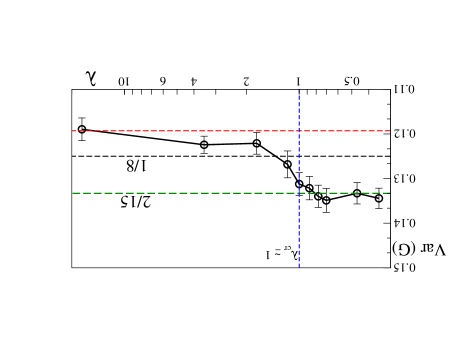
Figure 4: (colour online) ${\rm Var}(G)$ versus $\lambda$ for $n=7$, $m=14$, $N=3432$ and $M=20$ channels for the many-body model (1).

One can see from Fig. 4 that the variance ${\rm Var}(G)$ increases when $\lambda$ and $\mu$ decrease, and crosses the ballistic value $2/15$ close to the critical value at which the transition from weak to strong chaos occurs in closed models.

One of the most interesting and new results of our study is how the internal chaos influences the variance of the conductance, ${\rm Var}(G)$. As one can see from Fig. 5, in the region with small or moderate continuum coupling, $\kappa\approx 0.1-0.5$, the value of ${\rm Var}(G)$ strongly depends on the strength of inter-particle interaction, $\lambda$, in the model (1) of many-body chaos, and on the perturbation parameter $\mu$ in the model (3) of one-body chaos. The strongest influence of chaos occurs for $\kappa\approx 0.2$, and the results are practically the same for both models, provided the appropriate normalisation of $\lambda$ and $\mu$ is made. This important result may find various applications in theory of conductance fluctuations. In particular, one may try to extract information about internal dynamics from experimental data when changing the degree of coupling to continuum (for example, the degree of openness of quantum dots).

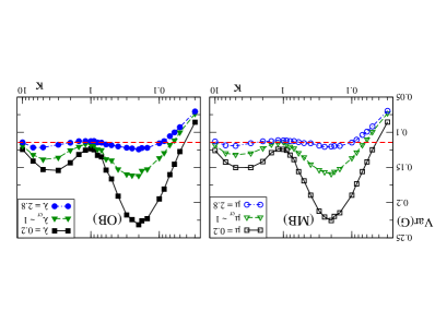
Figure 5: (colour online) Variance of the conductance for the many-body model (3), left panel, as compared to the one-body model, right panel. The average was done over 700 realisations of random matrices with $N=924$ and $M=10$.

An important feature of the data in Fig. 5 is that for $\kappa\approx 1$ the influence of intrinsic chaos is weak. This can be explained as follows. When coupling is perfect, an interaction with the continuum through forming broad states in various channels is very strong in comparison with an internal process of chaotization, therefore, the latter may be neglected. We found that for $\kappa\approx 1$ the sensitivity of the conductance fluctuations to the degree of chaos decreases with an increase of number of channels $M$.

It is instructive to show that the main properties of conductance fluctuations cannot be explained if one neglects cross section correlations discussed above. For the first time, the role of these correlations in application to conductance fluctuations has been discussed in Refs. [30, 31, 32]. The variance ${\rm Var}(G)$ can be rewritten as

$${\rm Var}(G)=\frac{M^{2}}{4}\left(\frac{T}{F+M-1}\right)^{2}+N_{1}C_{1}+N_{0}C_{0},$$ (13)

where $N_{1}=L(M-2),\,N_{0}=L(L-M+1),\,L=M^{2}/4$ and the terms $C_{1}$ and $C_{0}$ stand for the $II_{1}$ and $II_{0}$ correlation functions, respectively, see above. If one neglects the correlations, the first term gives $1/4$ (for $T=1$ and $M\gg 1$), instead of $1/8$. Our analysis shows that for the strong interaction and $M\gg 1$ one obtains $C_{1}\approx-M^{-3}$ and $C_{0}\approx 2M^{-4}$. Therefore, in the limit of a large number of channels, the first term in r.h.s. of Eq. (13) that equals $1/4$, is cancelled by the second term, and the third term tends to $1/8$ resulting in ${\rm Var}(G)=1/8$.

This result clearly demonstrates the crucial role of correlations determining the conductance fluctuations (see, also, Ref. [28]). Remarkably, the $II_{1}$-correlations cancel the first term $1/4$, and the value $1/8$ is due to the $II_{0}$-correlations (term $C_{0}$) only. A highly non-trivial role of the $C_{1}$ and $C_{0}$ terms can be also manifested in the correlations of speckle pictures [31].

6 Conclusions

To conclude, we studied the interplay of complicated intrinsic dynamics and coupling to the outside world for typical quantum systems with one-body or many-body intrinsic chaos, the first one coming from the disordered single-particle spectrum and the second one emerging as a result of inter-particle interactions. The openness of the system is described by the effective non-Hermitian Hamiltonian that fully respects the unitarity requirements and allows to calculate, in the same framework, cross sections of various processes, their fluctuations and correlations. As a manifestation of the general features of underlying physics, the models are equally valid for description of nuclear reactions with the transition from isolated to overlapping resonances and for conductance fluctuations in mesoscopic condensed matter devices. We found that the correlations of inelastic cross sections are very different for the processes with and without a common channel, being negative in the latter case in the region of perfect coupling when the typical decay widths and resonance spacings are of the same magnitude. Another important result is that for the conductance fluctuations the dependence on the degree of intrinsic chaos is strong at intermediate continuum coupling, in contrast with the region of perfect coupling, for which the continuum dominates, and the fluctuations are known to be independent of internal dynamics. Many results of the conductance theory are numerically confirmed being explained by the specific correlations of partial cross sections of very general origin.

- [1] \NameP.A. Mello N. Kumar \BookQuantum Transport in Mesoscopic Systems: Complexity and Statistical Fluctuations \PublOxford University Press, Oxford \Year2004.
- [2] \Name T.A. Brody, J. Flores, J.B. French, P.A. Mello, A. Pandey S.S.M. Wong \REVIEWRev. Mod. Phys.531981385.
- [3] \Name V.V. Flambaum, A.A. Gribakina, G.F. Gribakin, and M.G. Kozlov \REVIEWPhys. Rev. A501994267.
- [4] \NameV. Zelevinsky, B.A. Brown, N. Frazier, and M. Horoi \REVIEWPhys. Rep276199685.
- [5] \NameT. Guhr, A. Müller-Groeling, and H.A.Weidenmüller \REVIEWPhys. Rep.2991998189.
- [6] \NameT. Papenbrock and H.A. Weidenmüller \REVIEW Rev. Mod. Phys. 792007997.
- [7] \NameV.V. Flambaum and F.M. Izrailev \REVIEWPhys. Rev. E5619975144.
- [8] \NameS. Aberg \REVIEWPhys. Rev. Lett.2619903119.
- [9] \NameB.L. Altshuler, Y. Gefen, A. Kamenev and L.S. Levitov \REVIEWPhys. Rev. Lett.7819972803.
- [10] \NameT. Ericson \REVIEWAnn. Phys.231963390; \NameD. Brink and R. Stephen \REVIEWPhys. Lett.5196377; \NameT. Ericson and T. Mayer-Kuckuk \REVIEWAnn. Rev. Nucl. Sci.161966183.
- [11] \NameH. Feshbach \REVIEWAnn. Phys.51958357; \REVIEWAnn. Phys.191962287; \REVIEWRev. Mod. Phys. 3619641076.
- [12] \NameC. Mahaux and H.A. Weidenmüller \BookShell Model Approach to Nuclear Reactions \PublNorth Holland, Amsterdam \Year1969.
- [13] \NameV. V. Sokolov and V. G. Zelevinsky \REVIEWPhys. Lett. B 202199810; \REVIEWNucl. Phys.A5041989562 (1989); \REVIEWAnn. Phys. (N.Y.)2161992323.
- [14] \NameR.H. Dicke \REVIEWPhys. Rev.93195499.
- [15] \NameC.W.J. Beenakker \REVIEWRev. Mod. Phys.691997731.
- [16] \NameY. Imry R. Landauer \REVIEWRev. Mod. Phys.711999S306.
- [17] \NameH.A. Weidenmüller \REVIEWNucl. Phys.A51819901.
- [18] \NameG.L. Celardo, F.M. Izrailev, V.G. Zelevinsky G.P. Berman \REVIEWPhys. Rev. E762007031119; \REVIEWPhys. Lett. B6592008170.
- [19] \NameA. Volya V. Zelevinsky \REVIEWPhys. Rev. C742006064314; \REVIEWPhys. Rev. Lett.942005052501.
- [20] \NameD. Agassi, H.A. Weidenmüller, G. Mantzouranis \REVIEWPhys. Rep.31975145.
- [21] \NameJ.J.M. Verbaarschot, H.A. Weidenmüller, M.R. Zirnbauer \REVIEWPhys. Rep.1291985367.
- [22] \NameI. Rotter \REVIEWRep. Prog. Phys.541991635.
- [23] \NameF.M. Izrailev, D. Sacher V.V. Sokolov \REVIEWPhys. Rev. E491994130.
- [24] \NameF. Haake et al. \REVIEWZ. Phys. B 881992359.
- [25] \NameG.L. Celardo, F.M. Izrailev, S. Sorathia, V.G. Zelevinsky, G.P. Berman \BookNuclei and Mesoscopic Physics 2007 \EditorP. Danielewicz, P. Piecuch, V. Zelevinsky, \REVIEWAIP Conference Proceedings995200875.
- [26] \NameP.A.Mello A.D.Stone \REVIEWPhys. Rev. B4419913559.
- [27] \NameE.D. Davis D. Boose \REVIEWZ. Phys.A3321989427.
- [28] \NameA. García-Martín, F. Scheffold, M. Nieto-Vesperinas, J.J. Sáenz \REVIEWPhys. Rev. Lett.882002143901.
- [29] \NameH.L. Harney, A. Richter, H.A. Weidenmüller \REVIEWRev. Mod. Phys.581986607.
- [30] \NameP.A.Lee, A.S.Stone, H.Fukuyama \REVIEWPhys. Rev. B3519871039.
- [31] \NameS.Feng, C.Kane, P.A.Lee, A.D.Stone \REVIEWPhys. Rev. Lett.611988834; \NameI.Freud, M.Rosenbluth, S.Feng \REVIEWibid6119882328.
- [32] \NameP.A.Mello, E.Akkermans, B.Shapiro \REVIEWPhys. Rev. Lett.611988459.