Equatorial magnetic helicity flux in simulations with different gauges

Abstract

We use direct numerical simulations of forced MHD turbulence with a forcing function that produces two different signs of kinetic helicity in the upper and lower parts of the domain. We show that the mean flux of magnetic helicity from the small-scale field between the two parts of the domain can be described by a Fickian diffusion law with a diffusion coefficient that is approximately independent of the magnetic Reynolds number and about one third of the estimated turbulent magnetic diffusivity. The data suggest that the turbulent diffusive magnetic helicity flux can only be expected to alleviate catastrophic quenching at Reynolds numbers of more than several thousands. We further calculate the magnetic helicity density and its flux in the domain for three different gauges. We consider the Weyl gauge, in which the electrostatic potential vanishes, the pseudo-Lorenz gauge, where the speed of light is replaced by the sound speed, and the ‘resistive gauge’ in which the Laplacian of the magnetic vector potential acts as resistive term. We find that, in the statistically steady state, the time-averaged magnetic helicity density and the magnetic helicity flux are the same in all three gauges.

1 Introduction

The generation of magnetic fields on scales larger than the eddy scale of the underlying turbulence in astrophysical bodies has posed a major problem. Magnetic helicity is believed to play an important role in this process [(Brandenburg & Subramanian 2005a)]. The magnetic helicity density, defined by ${\bm{A}}\cdot{\bm{B}}$, where ${\bm{B}}={\bm{\nabla}}\times{\bm{A}}$ is the magnetic field and ${\bm{A}}$ is the corresponding magnetic vector potential, is important because at large scales it is produced in many dynamos. This has been demonstrated for dynamos based on the $\alpha$ effect ([Shukurov et al. 2006, Brandenburg et al. 2009]), the shear–current effect [(Brandenburg & Subramanian 2005b)], and the incoherent $\alpha$–shear effect [(Brandenburg et al. 2008)]. The volume integral of the magnetic helicity density over periodic domains (as well as domains with perfect-conductor boundary conditions or infinite domains where the magnetic field and the vector potential decays fast enough at infinity) is a conserved quantity in ideal MHD. This conservation is also believed to be recovered in the limit of infinite magnetic Reynolds number in non-ideal MHD [(Berger 1984)]. This implies that for finite (but large) magnetic Reynolds numbers magnetic helicity can decay only through microscopic resistivity. This would in turn control the saturation time and cycle periods of large-scale helical magnetic field which would be too slow to explain the observed variations of magnetic fields in astrophysical settings, such as for example the 11 year variation of the large-scale fields during the solar cycle.

A possible way out of this deadlock is provided by fluxes of magnetic helicity out of the domain ([Blackman & Field 2000, Kleeorin et al. 2000]). In the case of solar dynamo, such a flux could be out of the domain, mediated by coronal mass ejections, or it could be across the equator, mediated by internal fluxes within the domain. Several possible candidates for magnetic helicity fluxes have been proposed ([Kleeorin & Rogachevskii 1999, Vishniac & Cho 2001, Subramanian & Brandenburg 2004]).

In this paper we measure the diffusive flux across the domain with two different signs of magnetic helicity. This measurement however poses an additional difficulty, due to the fact that neither the flux nor the magnetic helicity density remain invariant under the gauge transformation ${\bm{A}}\rightarrow{\bm{A}}+\mbox{\boldmath$\nabla$}{}\Lambda$, up to which the vector potential is defined. This constitutes a gauge problem. This problem, however, does not arise in homogeneous (or nearly homogeneous) domains with periodic or perfect-conductor boundary conditions, or in infinitely large domains where both the magnetic field and vector potential decay fast enough at infinity. In these cases the volume integral of magnetic helicity is gauge-invariant, because surface terms vanish and $\mbox{\boldmath$\nabla$}{}\cdot{\bm{B}}=0$, so that $\int{\bm{B}}\cdot\mbox{\boldmath$\nabla$}{}\Lambda\,{\rm d}{}V=-\int\Lambda\mbox{\boldmath$\nabla$}{}\cdot{\bm{B}}\,{\rm d}{}V=0$. However, in practice we are often interested in finite or open domains with more realistic boundary conditions. Also, if we are to talk meaningfully about the exchange of magnetic helicity between two parts of the domain we need to evaluate changes in magnetic helicity densities locally even if the integral of the magnetic helicity density over the whole domain is gauge-invariant. An important question then is how to calculate this quantity across arbitrary surfaces in numerical simulations. Ideally one would like to have a gauge-invariant description of magnetic helicity. A number of suggestions have been put forward in the literature ([Berger & Field 1984, Subramanian & Brandenburg 2006]). In practice, however, calculating the gauge-invariant volume integral of magnetic helicity poses an awkward complication and may not be the quantity relevant for dynamo quenching ([Subramanian & Brandenburg 2006]). In this paper, to partially address this question, we take an alternative view and try to compare and contrast the magnetic helicity and its flux across the domain in three different gauges that are often used in numerical simulations.

2 Model and Background

The setup in this paper is inspired by the recent work of [Mitra et al. (2009)], who considered a wedge-shaped domain encompassing parts of both the southern and northern hemispheres. Direct numerical simulations (DNS) of the compressible MHD equations with an external force which injected negative (positive) helicity in the northern (southern) hemispheres shows a dynamo with polarity reversals, oscillations and equatorward migration of magnetic activity. It was further shown, using mean-field models, that such a dynamo is well described by an $\alpha^{2}$ dynamo, where $\alpha$ has positive (negative) sign in the northern (southern) hemisphere. However, the mean-field dynamo showed catastrophic quenching, i.e., the ratio of magnetic energy to the equipartition magnetic energy decreases as $R_{\rm m}^{-1}$, where $R_{\rm m}$ is the magnetic Reynolds number. Such catastrophic quenching could potentially be alleviated by a mean flux of small-scale magnetic helicity across the equator ([Brandenburg et al. 2009]). Diffusive flux of this kind has previously been employed in mean-field models on empirical grounds ([Covas et al. 1998, Kleeorin et al. 2000]). Using a one-dimensional mean-field model of an $\alpha^{2}$ dynamo with positive $\alpha$ in the north and negative in the south, it was possible to show that for large enough values of $R_{\rm m}$ catastrophic quenching is indeed alleviated ([Brandenburg et al. 2009]). However, three questions still remained:

1. Can such a diffusive flux result from DNS?

2. Is it strong enough to alleviate catastrophic quenching?

3. When is it independent of the gauge chosen?

In this paper we provide partial answers to these questions.

We proceed by simplifying our problem further, both conceptually and numerically, by considering simulations performed in a rectangular Cartesian box with dimensions $L_{x}\times L_{y}\times L_{z}$. The box is divided into two equal cubes along the $z$ direction, with sides $L_{x}=L_{y}=L_{z}/2$. We shall refer to the $xy$ plane at $z=0$ as the ‘equator’ and the regions with positive (negative) $z$ as ‘north’ and ‘south’ respectively. We shall choose the helicity of the external force such that it has negative (positive) helicity in the northern (southern) parts of the domain. All the sides of the simulation domain are chosen to have periodic boundary conditions. The slowest resistive decay rate of the mean magnetic field is $\eta k_{1}^{2}$, where $\eta$ is the microscopic magnetic diffusivity and $k_{1}=\pi/L_{z}$ is the lowest wavenumber of the domain.

We employ two different random forcing functions: one where the helicity of the forcing function varies sinusoidally with $z$ (Model A) and one where it varies linearly with $z$ (Model B). This also leads to a corresponding variation of the kinetic and small-scale current helicities in the domain. Model A minimizes the possibility of boundary effects, while Model B employs the same profile as that used in an earlier mean-field model ([Brandenburg et al. 2009]). The typical wavenumber of the forcing function is chosen to be $k_{\rm f}=20k_{1}$ in Model A and $k_{\rm f}=16k_{1}$ in Model B. An important control parameter of our simulations is the magnetic Reynolds number, $R_{\rm m}=u_{\rm rms}/\eta k_{\rm f}$, which is varied between 2 and 68, although we also present a result with a larger value of $R_{\rm m}$. This last simulation may not have run long enough and will therefore not be analyzed in detailed.

We perform DNS of the equations of compressible MHD for an isothermal gas with constant sound speed $c_{\rm s}$,

$$D_{t}{\bm{U}} = -c_{\rm s}^{2}{\bm{\nabla}}\ln\rho+\frac{1}{\rho}{\bm{J}}\times{\bm{B}}+\bm{F}_{\rm visc}+{\bm{f}},$$ (1)

$$D_{t}\ln\rho = -{\bm{\nabla}}\cdot{\bm{U}},$$ (2)

$$\partial_{t}{\bm{A}} = {\bm{U}}\times{\bm{B}}-\eta\mu_{0}{\bm{J}}-{\bm{\nabla}}\psi,$$ (3)

where $\bm{F}_{\rm visc}=(\mu/\rho)(\nabla^{2}{\bm{U}}+\frac{1}{3}{\bm{\nabla}}{\bm{\nabla}}\cdot{\bm{U}})$ is the viscous force when the dynamic viscosity $\mu$ is constant (Model A), and $\bm{F}_{\rm visc}=\nu(\nabla^{2}{\bm{U}}+\frac{1}{3}{\bm{\nabla}}{\bm{\nabla}}\cdot{\bm{U}}+2\mbox{\boldmath${\sf S}$}{}\ln\rho)$ is the viscous force when the kinematic viscosity $\nu$ is constant (Model B), ${\bm{U}}$ is the velocity, ${\bm{J}}={\bm{\nabla}}\times{\bm{B}}/\mu_{0}$ is the current density, $\mu_{0}$ is the vacuum permeability (in the following we measure the magnetic field in Alfvén units by setting $\mu_{0}=1$ everywhere), $\rho$ is the density, $\psi$ is the electrostatic potential, and $D_{t}\equiv\partial_{t}+{\bm{U}}\cdot{\bm{\nabla}}$ is the advective derivative. Here ${\bm{f}}({\bm{x}},t)$ is an external random white-in-time helical function of space and time. The simulations were performed with the Pencil Code, which uses sixth-order explicit finite differences in space and third order accurate time stepping method. We use a numerical resolution of $128\times 128\times 256$ meshpoints.

These simulations in a Cartesian box capture the essential aspects of the simulations of [Mitra et al. (2009)] in spherical wedge-shaped domains. In particular, in this case we also observe the generation of large-scale magnetic fields which show oscillations on dynamical time scales, reversals of polarity and equatorward migration, as can be seen from the sequence of snapshots in Fig. 1 for a run with $R_{\rm m}=68$. Here we express time in units of the expected turbulent diffusion time, $T=(\eta_{\rm t0}k_{1}^{2})^{-1}$, where $\eta_{\rm t0}=u_{\rm rms}/3k_{\rm f}$ is used as reference value [(Sur et al. 2008)].

Below we shall employ this setup to study the magnetic helicity and its flux. We shall discuss the issue of gauge-dependence in Sect. 5.

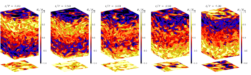
Figure 1: Visualization of the $B_{y}$ component of the magnetic field on the periphery of the domain at different times showing the migration of magnetic patterns from the top and bottom boundaries toward the equator. Time is measured in turbulent diffusion times, $T=(\eta_{\rm t0}k_{1}^{2})^{-1}$, where $\eta_{\rm t0}=u_{\rm rms}/3k_{\rm f}$ is used as reference

3 Magnetic helicity fluxes

Let us first summarize the role played by magnetic helicity and its fluxes in large-scale helical dynamos. The simplest case is that of a closed domain, i.e., one with periodic or perfect-conductor boundary conditions. In the spirit of mean-field theory, we define large-scale (or mean) quantities, denoted by an overbar, as a horizontal average taken over the $x$ and $y$ directions. In addition, we denote a volume average by angular brackets, $\langle\cdot\rangle$. The magnetic helicity density is denoted by

$$h^{\rm M}\equiv{\bm{A}}\cdot{\bm{B}},$$ (4)

and its integral over a volume $V$ is denoted by

$$H^{\rm M}\equiv\langle h^{\rm M}\rangle\equiv\frac{1}{V}\int_{V}{\bm{A}}\cdot{\bm{B}}\,{\rm d}{}V.$$ (5)

In general the evolution equation of $h^{\rm M}$ can be written down using the MHD equations, which yields

$$\partial_{t}h^{\rm M}=-2{\bm{E}}\cdot{\bm{B}}-{\bm{\nabla}}\cdot{\mbox{\boldmath${\cal F}$}}^{\rm H},$$ (6)

where

$${\mbox{\boldmath${\cal F}$}}^{\rm H}={\bm{E}}\times{\bm{A}}+\psi{\bm{B}}$$ (7)

is the magnetic helicity flux and ${\bm{E}}$ is the electric field, which is given by

$${\bm{E}}=-{\bm{U}}\times{\bm{B}}+\eta{\bm{J}}.$$ (8)

Given that our system is statistically homogeneous in the horizontal directions, we consider the evolution equation for the horizontally averaged magnetic helicity density,

$$\partial_{t}\overline{h}^{\rm M}=-2\eta\overline{{\bm{J}}\cdot{\bm{B}}}-{\bm{\nabla}}\cdot\overline{\mbox{\boldmath${\cal F}$}}^{\rm H},$$ (9)

where the contribution from the full electromotive force, ${\bm{U}}\times{\bm{B}}$, has dropped out after taking the dot product with ${\bm{B}}$. However, the mean electromotive force from the fluctuating fields, $\overline{\mbox{\boldmath${\cal E}$}}=\overline{{\bm{u}}\times{\bm{b}}}$, enters the evolution of the mean fields, so this contribution does not vanish if we consider separately the contributions to $\overline{h}^{\rm M}$ that result from mean and fluctuating fields, i.e.

$$\partial_{t}\overline{h}^{\rm M}_{\rm m}=2\overline{\mbox{\boldmath${\cal E}$}}\cdot{\overline{\bm{B}}}-2\eta{\overline{\bm{J}}}\cdot{\overline{\bm{B}}}-{\bm{\nabla}}\cdot\overline{\mbox{\boldmath${\cal F}$}}^{\rm H}_{\rm m},$$ (10)

$$\partial_{t}\overline{h}^{\rm M}_{\rm f}=-2\overline{\mbox{\boldmath${\cal E}$}}\cdot{\overline{\bm{B}}}-2\eta\overline{{\bm{j}}\cdot{\bm{b}}}-{\bm{\nabla}}\cdot\overline{\mbox{\boldmath${\cal F}$}}^{\rm H}_{\rm f},$$ (11)

where

$$\overline{\mbox{\boldmath${\cal F}$}}^{\rm H}_{\rm m} = {\overline{\bm{E}}}\times{\overline{\bm{A}}}+\overline{\Psi}\,\overline{{\bm{B}}},$$ (12)

$$\overline{\mbox{\boldmath${\cal F}$}}^{\rm H}_{\rm f} = \overline{{\bm{e}}\times{\bm{a}}}+\overline{\psi{\bm{b}}},$$ (13)

and $\Psi=\overline{\Psi}+\psi$.

In mean-field dynamo theory one solves the evolution equation for $\overline{{\bm{B}}}$, so $\overline{\mbox{\boldmath${\cal F}$}}^{\rm H}_{\rm m}$ is known explicitly from the actual mean fields. However, the evolution equation for $\overline{h}^{\rm M}_{\rm f}$ is not automatically obeyed in the usual mean-field treatment. This is the reason why in the dynamical quenching formalism this equation is added as an additional constraint equation. The terms $\overline{h}^{\rm M}_{\rm f}$ and $\overline{{\bm{j}}\cdot{\bm{b}}}\approx k_{\rm f}^{2}\overline{h}^{\rm M}_{\rm f}$ are coupled to the mean-field equations through an additional contribution to the $\alpha$ effect with a term proportional to $k_{\rm f}^{2}\overline{h}^{\rm M}_{\rm f}$. However, the coupling of the flux term $\overline{\mbox{\boldmath${\cal F}$}}^{\rm H}_{\rm f}$ is less clear, because there are several possibilities and their relative importance is not well established.

In this paper we are primarily interested in $\overline{\mbox{\boldmath${\cal F}$}}^{\rm H}_{\rm f}$ across the equator. We assume that this flux can be written in terms of the gradient of the magnetic helicity density via a Fickian diffusion law, i.e.,

$$\overline{\mbox{\boldmath${\cal F}$}}^{\rm H}_{\rm f}=-\kappa_{\rm f}{\bm{\nabla}}\overline{h}^{\rm M}_{\rm f},$$ (14)

where $\kappa_{\rm f}$ is an effective diffusion coefficient for the magnetic helicity density.

There are several points to note regarding Eq. (14). Firstly, both the magnetic helicity and its flux are gauge-dependent. Hence this expression should in principle depend on the gauge we choose. However, as catastrophic quenching is a physically observable phenomenon, it should not depend on the particular gauge chosen. Secondly, we recall that Eq. (14) is purely a conjecture at this stage, and it is the aim of this paper to test this conjecture. Thirdly, Eq. (14) is not the only form of flux of magnetic helicity possible. Two other obvious candidates are the advective flux and the Vishniac–Cho flux ([Vishniac & Cho 2001]). However, none of them can be of importance to the problem at hand, because we have neither a large-scale velocity (thus ruling out advective flux) nor a large-scale shear (thus ruling out Vishniac–Cho flux).

4 Diffusive flux and $R_{\rm m}$ dependence

Let us postpone the discussion of the complications arising from the choice of gauge until Sect. 5 and use the resistive gauge for the results reported in this section, i.e. we set

$$\psi=\eta{\bm{\nabla}}\cdot{\bm{A}}.$$ (15)

We then calculate ${\overline{\cal F}}^{\rm H}_{\rm f}$ and $\overline{h}^{\rm M}_{\rm f}$ as functions of $z$ from our simulations, time-average both of them and use Eq. (14) to calculate $\kappa_{\rm f}$ from a least-square fit of ${\overline{\cal F}}^{\rm H}_{\rm f}$ versus $-\mbox{\boldmath$\nabla$}{}\overline{h}^{\rm M}_{\rm f}$ within the range $-1.3\leq k_{1}z\leq 1.3$. The values of $\kappa_{\rm f}$ as a function of $R_{\rm m}$ is given in the last column of Table LABEL:TermsRHS.

In order to determine the relative importance of equatorial magnetic helicity fluxes, we now consider individually the three terms on the RHS of Eq. (11). Within the range $-1.3\leq k_{1}z\leq 1.3$, all three terms vary roughly linearly with $z$. We therefore determine the slope of this dependence. In Table LABEL:TermsRHS we compare these three terms at $k_{1}z=-1$, evaluated in units of $\eta_{\rm t0}k_{1}B_{\rm eq}^{2}$, as well as the value of $\kappa_{\rm f}/\eta_{\rm t0}$. In Fig. 2 we show the $z$ dependence of these three terms for Run B5, where $R_{\rm m}=68$. The values of $\kappa_{\rm f}$ as a function of $R_{\rm m}$ is given in the last column of Table LABEL:TermsRHS. The $z$ dependence of ${\overline{\cal F}}^{\rm H}_{\rm f}$ and $\overline{h}^{\rm M}_{\rm f}$ is shown in the last panel of Fig. 2. Note that the two profiles agree quite well.

Table 1: Dependence of ${\overline{\bm{B}}}^{2}$, normalized by $B_{\rm eq}^{2}$, the slopes of the three terms on the RHS of Eq. (11), normalized by $\eta_{\rm t0}B_{\rm eq}^{2}$, as well as the value of $\kappa_{\rm f}/\eta_{\rm t0}$.

Run $R_{\rm m}$ ${\overline{\bm{B}}}^{2}$ $2\overline{\mbox{\boldmath${\cal E}$}}\cdot\overline{\bm{B}}$ $2\eta\overline{{\bm{j}}\cdot{\bm{b}}}$ ${\bm{\nabla}}\cdot\overline{\mbox{\boldmath${\cal F}$}}^{\rm H}_{\rm f}$ $\kappa_{\rm f}/\eta_{\rm t0}$ B1 2 1.1 9.42 $-9.38$ $-0.04$ 0.41 B2 5 2.2 11.18 $-11.14$ $-0.04$ 0.34 B3 15 2.0 4.54 $-4.52$ $-0.02$ 0.27 B4 33 1.7 2.28 $-2.27$ $-0.01$ 0.31 B5 68 0.8 1.15 $-1.12$ $-0.03$ 0.34

Figure 2: $z$ dependence of the terms on the RHS of Eq. (11) in the first two panels and in Eq. (14) for Run B5.

We point out that, near $z=0$, all simulations show either a local reduction in the gradients of the terms on the RHS of Eq. (11) or even a local reversal of the gradient. This is likely to be associated with a local reduction in dynamo activity near $z=0$, where kinetic helicity is zero. The non-uniformity of the turbulent magnetic field also leads to transport effects [(Brandenburg & Subramanian 2005a)] that may modify the gradient. However, we shall not pursue this question further here.

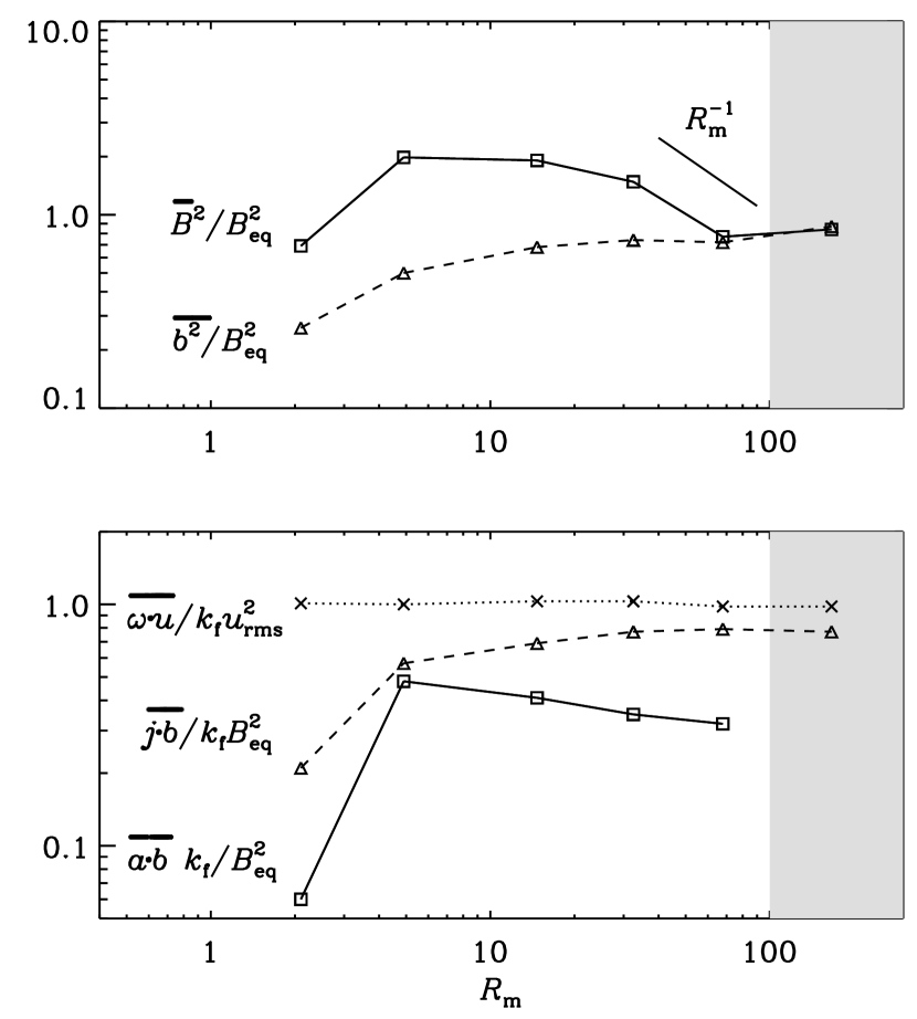
Figure 3: $R_{\rm m}$ dependence of the normalized magnetic energy of the mean field, $\langle\overline{\bm{B}}^{2}\rangle/B_{\rm eq}^{2}$, and the fluctuating field, $\langle{\bm{b}}^{2}\rangle/B_{\rm eq}^{2}$, in the upper panel together with the normalized helicities of the small-scale magnetic field, $\overline{{\bm{a}}\cdot{\bm{b}}}k_{\rm f}/B_{\rm eq}^{2}$, the small-scale current density, $\overline{{\bm{j}}\cdot{\bm{b}}}/k_{\rm f}B_{\rm eq}^{2}$, and the small-scale velocity, $\overline{\vec{\omega}\cdot{\bm{u}}}/k_{\rm f}u_{\rm rms}^{2}$, at $k_{1}z=-1$ (i.e. in the south) in the lower panel. (All three helicities are negative in the north and positive in the south.) The shaded ares indicates that the solutions are different in nature, and that the simulations may not have run for long enough.

Looking at Table LABEL:TermsRHS, we see that $2\overline{\mbox{\boldmath${\cal E}$}}\cdot\overline{\bm{B}}$ and $2\eta\overline{{\bm{j}}\cdot{\bm{b}}}$ balance each other nearly perfectly, and that only a small residual is then balanced by the diffusive flux divergence, ${\bm{\nabla}}\cdot\overline{\mbox{\boldmath${\cal F}$}}^{\rm H}_{\rm f}$. For the values of $R_{\rm m}$ considered here, the terms $2\overline{\mbox{\boldmath${\cal E}$}}\cdot\overline{\bm{B}}$ and $2\eta\overline{{\bm{j}}\cdot{\bm{b}}}$ scale with $R_{\rm m}$, while the dependence of ${\bm{\nabla}}\cdot\overline{\mbox{\boldmath${\cal F}$}}^{\rm H}_{\rm f}$ on $R_{\rm m}$ is comparatively weak. If catastrophic quenching is to be alleviated by the magnetic helicity flux, one would expect that at large values of $R_{\rm m}$ the terms $2\overline{\mbox{\boldmath${\cal E}$}}\cdot\overline{\bm{B}}$ and ${\bm{\nabla}}\cdot\overline{\mbox{\boldmath${\cal F}$}}^{\rm H}_{\rm f}$ should balance. At the moment our values of $R_{\rm m}$ are still too small by about a factor of 30-60 (assuming that the same scaling with $R_{\rm m}$ persists). This result is compatible with that of earlier mean field models ([Brandenburg et al. 2009]). Consequently, we see that the energy of the mean magnetic field decreases with increasing from $R_{\rm m}=33$ to 68; see Fig. 3. For larger values of $R_{\rm m}$ the situation is still unclear.

In Table LABEL:TermsRHS, we also give the approximate values of $\kappa_{\rm f}/\eta_{\rm t0}$. Note that this ratio is always around 0.3 and independent of $R_{\rm m}$. This is the first time that an estimate for the diffusion coefficient of the diffusive flux has been obtained. There exists no theoretical prediction for value of $\kappa_{\rm f}$ other than the naive expectation that such a term should be expected and that its value should be of the order of $\eta_{\rm t0}$. This now allows us to state more precisely the point where the turbulent diffusive helicity flux becomes comparable with the resistive term, i.e. we assume $\kappa_{\rm f}\nabla^{2}\overline{{\bm{a}}\cdot{\bm{b}}}$ to become comparable with $2\eta\overline{{\bm{j}}\cdot{\bm{b}}}$. Using the relation $\overline{{\bm{j}}\cdot{\bm{b}}}\approx k_{\rm f}^{2}\overline{{\bm{a}}\cdot{\bm{b}}}$ [(Blackman & Brandenburg 2002)], which is confirmed by the current simulations within a factor of about 2 (see the second panel of Fig. 3), we find that

$$\kappa_{\rm f}/2\eta>(k_{\rm f}/k_{1})^{2},$$ (16)

where we have assumed that the Laplacian of $\overline{{\bm{a}}\cdot{\bm{b}}}$ can be replaced by a $k_{1}^{2}$ factor. Using our empirical finding, $\kappa_{\rm f}\approx\eta_{\rm t0}/3$, together with the definition $\eta_{\rm t0}/\eta\approx u_{\rm rms}/3\eta k_{\rm f}=R_{\rm m}/3$, we arrive at the condition

$$R_{\rm m}>18(k_{\rm f}/k_{1})^{2}\approx 4600\quad\mbox{(for $\kappa_{\rm f}$ to be important)},$$ (17)

where we have inserted the value $k_{\rm f}/k_{1}=16$ for the present simulations. Similarly, large values of $R_{\rm m}$ for alleviating catastrophic quenching by turbulent diffusive helicity fluxes were also found using mean-field modelling ([Brandenburg et al. 2009]). Unfortunately, the computing resources are still not sufficient to verify this in the immediate future.

5 Gauge-dependence of helicity flux

Let us now consider the question of gauge-dependence of the helicity flux. Equation (11) is obviously gauge-dependent. However, if, in the statistically steady state, $\overline{h}^{\rm M}_{\rm f}$ becomes independent of time, we can average this equation and obtain

$${\partial{\overline{\cal F}}^{\rm H}_{\rm f}\over\partial z}=-2\overline{\mbox{\boldmath${\cal E}$}}\cdot\overline{\bm{B}}-2\eta\overline{{\bm{j}}\cdot{\bm{b}}},$$ (18)

where ${\overline{\cal F}}^{\rm H}_{\rm f}$ refers to the $z$ component of $\overline{\mbox{\boldmath${\cal F}$}}^{\rm H}_{\rm f}$. On the RHS of this equation the two terms are gauge-independent. Therefore ${\bm{\nabla}}\cdot{\overline{\cal F}}^{\rm H}_{\rm f}$ must also be gauge-independent. The same applies also to ${\overline{\cal F}}^{\rm H}_{\rm m}$ and $\overline{\cal F}^{\rm H}$; see Eq. (9). We have confirmed that, in the steady state, $\overline{h}^{\rm M}_{\rm f}$ is statistically steady and does not show a long-term trend; cf. Fig. 4 for the three gauges. We note that the fluctuations of $\overline{h}^{\rm M}_{\rm f}$ are typically much larger for the Weyl gauge than for the other two.

We now verify the expected gauge-independence explicitly for three different gauges: the Weyl gauge, defined by

$$\psi=0,$$ (19)

the Lorenz gauge (or pseudo-Lorenz gauge), defined by

$$\partial_{t}\psi=-c^{2}_{\psi}{\bm{\nabla}}\cdot{\bm{A}},$$ (20)

and the resistive gauge, defined by (15) above. We calculate the normalized magnetic helicity for both the mean and fluctuating parts and the respective fluxes for all the three gauges. These simulations are done for the Model A with low $R_{\rm m}$ ($R_{\rm m}\approx 1.9$).

We find the transport coefficient $\kappa_{\rm f}$ in the way described in the previous section. A snapshot of the mean flux ${\overline{\cal F}}^{\rm H}_{\rm f}$ is plotted in the top panel of Fig. 5. The flux is different in all the three gauges. However, when averaged over the horizontal directions as well as time the fluxes in the three different gauges agree with one another as shown in the bottom panel of Fig. 5. We find the transport coefficient $\kappa_{\rm f}$ as described in the previous section and obtain the same value in all the three gauges.

Figure 4: Plot of $\overline{h}^{\rm M}_{\rm f}$ as a function of time in the statistically stationary state for $k_{1}z=-1$ (south, top panel) and $k_{1}z=1$ (north, bottom panel) for the three different gauges, Weyl gauge (open circle), Lorenz gauge (line) and resistive gauge (broken line).

Figure 5: Comparison of the flux ${\overline{\cal F}}^{\rm H}_{\rm f}(z,t)$ at a randomly chosen instant (upper panel) and its time average ${\overline{\cal F}}^{\rm H}_{\rm f}(z)$ for the three different gauges. Lorenz gauge ($\circ$), Weyl gauge ($\diamond$) and the resistive gauge ($\cdot$). The instantaneous flux is plotted in the top panel and the time-averaged flux is plotted in the bottom panel.

6 Conclusion

In this paper we use a setup in which the two parts of the domain have different signs of kinetic and magnetic helicities. Using DNS we show that the flux of magnetic helicity due to small-scale fields can be described by Fickian diffusion down the gradient of this quantity. The corresponding diffusion coefficient is approximately independent of $R_{\rm m}$. However, in the range of $R_{\rm m}$ values we have considered here, the flux is not big enough to alleviate the catastrophic quenching. The critical value of $R_{\rm m}$ for the flux to become important is proportional to the square of the scale separation ratio. In the present case, where this ratio is 16, the critical value of $R_{\rm m}$ is estimated to be 4600. We have also calculated the flux and the diffusion coefficient in the three gauges discussed above and have found the fluxes to be independent of the choice of these gauges. This is explained by the fact that in the steady state the divergence of magnetic helicity flux is balanced by terms that are gauge-independent.

Several immediate improvements on this study spring to mind. One is to compare our results with the gauge-independent magnetic helicity of Berger & Field (1984) and the corresponding magnetic helicity flux. The second is to extend the present study to higher values of $R_{\rm m}$ to understand the asymptotic behavior of the flux. Finally, it may be useful to compare the results for different profiles of kinetic helicity to see whether or not our results depend on such details.