Hubbard fermions band splitting at the strong intersite Coulomb interaction

Abstract

The effect of the strong intersite Coulomb correlations on the formation of the electron structure of the $t-V$–model has been studied. A qualitatively new result has been obtained which consists in the occurrence of a split-off band of the Fermi states. The spectral intensity of this band increases with the enhancement of a doping level and is determined by the mean-square fluctuation of the occupation numbers. This leads to the qualitative change in the structure of the electron density of states.

PACS numbers

71.10.Fd, 71.18.+y, 71.27.+a, 71.28.+d, 71.70.-d

The key point of the theory of the strongly correlated electron systems is the statement on a principal role of the one-site Coulomb repulsion of two electrons with the opposite spin projections, e.g., the Hubbard correlations H63 , in the formation of the ground state and the elementary excitation spectrum Anderson . One of the brightest manifestations of the Hubbard correlations is splitting of the initial band of the energy spectrum into two Hubbard subbands when one-site energy of the Coulomb interaction $U$ exceeds the bandwidth $W$.

As was noted previously Rogdai1 ; Rogdai2 , when hole concentration in a system described by the Hubbard model is small and value $U$ is large the intersite Coulomb interaction starts playing an important role due to its relatively weak screening. In this case at distances close to interatomic the order of magnitude of characteristic value $V$ of the Coulomb interaction between electrons can be comparable with that of value $U$. Manifestation of the intersite correlations in the physical properties of systems has been considered in many works (see, for instance, Rogdai1 ; Rogdai2 ; Falicov ; Khomskii ; Matsukawa ; Littlewood ; Fedro ; Li ; Larsen ; Onishi ; Neudert ; Barreteau ; Miyake ). However, until recent time no attention has been paid to the fact that the strong intersite correlations (SIC) can cause splitting energy bands of the Fermi states into subbands VVMK .

Qualitatively, the physical origin of this phenomenon is similar to that of the occurrence of the Hubbard subbands due to the strong one-site correlations and is related to the fact that when the intersite Coulomb interactions are taken into account the energy of the electron located on site $f$ becomes dependent of the valence configuration of its nearest neighborhood. For example in the case of a lower Hubbard subband, if there is one electron on each of the $z$ nearest neighboring ions, the ”setting” energy of an electron is determined as a sum of one-site energy $\varepsilon$ and energy $zV$ of the interaction. If a hole appears in the nearest neighborhood, the ”setting” energy is $\varepsilon+(z-1)V$, i.e., its value is less than the previous one by $V$.

These simple arguments show that when configuration neighborhood deviates from nominal one, one should expect the occurrence of the states with the energies different by $V$ in the Fermi excitation spectrum. For the strongly correlated systems with a relatively narrow energy band of the Fermi states, the situation becomes possible when hopping parameter $t$ is commensurable with or less than $V$. Under these conditions splitting the initial band of the Fermi states is expected. Obviously, the more probable the deviation of the electron configuration of the neighborhood from the nominal one the higher is the spectral intensity of the split-off band. A quantitative measure of this deviation is a mean-square fluctuation of the occupation numbers. For this reason the split-off band was named the band of the fluctuation states (BFS) VVMK . For undoped Mott-Hubbard insulators the electron configuration of the neighborhood corresponds to the nominal one. Upon doping the deviation occurs and in the energy spectrum of the Fermi states the BFS appears whose spectral intensity increases with doping level. The aim of this Letter is to prove the presented qualitative interpretation.

In order to demonstrate the effect as brightly as possible we will consider the Hubbard model in the regime of the strong electron correlations ($U=\infty$) at electron concentrations $n\ll 1$. In this case the electron properties of the model are determined by the lower Hubbard subband. Considering the arguments presented in Rogdai1 ; Rogdai2 we will take into account the Coulomb interaction between the electrons located on the neighboring sites. The obtained system of the Hubbard fermions in the atomic representation will be described by the Hamiltonian of the $t-V$–model:

$$\hat{H}=\sum\limits_{f\sigma}\varepsilon_{0}X_{f}^{\sigma\sigma}+\sum\limits_{fm\sigma}t_{fm}X_{f}^{\sigma 0}X_{m}^{0\sigma}+\frac{V}{2}\sum\limits_{f\delta}\hat{n}_{f}\hat{n}_{f+\delta}.$$ (1)

Here the first term reflects an ensemble of noninteracting electrons in the Wannier representation. The occurrence a fermion with spin projection $\sigma$ at site $f$ increases the energy of the system by value $\varepsilon_{0}$, $X^{pq}_{f}=|f,p\rangle\langle f,q|$ are the Hubbard operators H65 ; SGOVV describing the transition from the one-site state $|q\rangle$ to the state $|p\rangle$. The second term corresponds to the kinetic energy of the Hubbard fermions where matrix element $t_{fm}$ determines the intensity of electron hopping from site $f$ to site $m$. The last term of the Hamiltonian takes into account the Coulomb interaction between the electrons located on neighboring sites $f$ and $f+\delta$ with intensity $V$. The operator of the number of electrons on site $f$ is $\hat{n}_{f}=\displaystyle\sum_{\sigma}X_{f}^{\sigma\sigma}$.

Below we limit our consideration to the case when the number of holes $h=(1/N)\sum_{f}\langle X_{f}^{00}\rangle$ in the system is small; i. e., the condition $h=1-n\ll 1$ is satisfied. In this regime it is reasonable to extract in explicit form the mean-field effects caused by the intersite interactions. Using the condition of completeness of the diagonal $X$-operators in the reduced Hilbert space $X^{00}_{f}+X^{\uparrow\uparrow}_{f}+X^{\downarrow\downarrow}_{f}=1$ we express Hamiltonian (1) as

$$\hat{H} = -E_{0}+\sum\limits_{f\sigma}\bigl{(}\varepsilon-4Vh\bigr{)}X_{f}^{\sigma\sigma}+\sum\limits_{fm\sigma}t_{fm}X_{f}^{\sigma 0}X_{m}^{0\sigma}$$ (2)

$$+\frac{1}{2}\sum_{f\delta}V\bigl{(}X^{00}_{f}-h\bigr{)}\bigl{(}X^{00}_{f+\delta}-h\bigr{)},$$

where $E_{0}=2NV(1-h)^{2}$ in the mean-field approximation determines the energy of the Coulomb interaction of the system containing $h$ holes per site. At $h=0$ value $E_{0}$ equals to the exact value of the energy of the ground state of the system (with disregard for $\varepsilon_{0}$), since in this case hoppings make no contribution. The renormalized value of a one-electron level $\varepsilon=\varepsilon_{0}+4V$ is determined by the fact that when there is one electron on each neighboring site the excitation energy increases by $4V$. The shift $\varepsilon-4hV$ is related to the decrease in the Coulomb repulsion energy when the average number of holes in the system is nonzero. Note that such mean-field renormalizations of the one-site energies of electrons were used previously, for example, in the Falicov–Kimball model during investigation of the transitions with the change in valence. Extraction of the obvious mean-field effects is needed for representation of the intersite interaction in the form containing the correlation effects only. One can see that the last term of the Hamiltonian (2) will contribute only at the presence of noticeable fluctuations of the occupation numbers, i. e., when the SICs are relatively large.

The method used below for the description of the strong intersite interactions (SII) consists in generalization of the Hubbard idea H63 for consideration of the intersite interactions VVMK . It follows from the exact equation of motion for operator $X_{f}^{0\sigma}$

$$i\frac{d}{dt}X^{0\sigma}_{f} =(\varepsilon-4Vh)X^{0\sigma}_{f}-V\sum_{\delta}X_{f}^{0\sigma}(X^{00}_{f+\delta}-h)$$ (3)

$$+\sum_{m}t_{fm}\bigl{(}(X_{f}^{00}+X_{f}^{\sigma\sigma})X_{m}^{0\sigma}+X_{f}^{\bar{\sigma}\sigma}X_{m}^{0\bar{\sigma}}\bigr{)},$$

that at large $V$ one should correctly consider the contributions related to the second term in the right part of equation (3). One of the ways of solving such a problem is to extend the basis set of operators by means of inclusion of the operators

$$\hat{\Phi}_{f}^{\sigma}=\sum_{\delta}X_{f}^{0\sigma}(X^{00}_{f+\delta}-h),$$ (4)

in which uncoupling is forbidden. This operator describes the correlated process of annihilation of an electron on site $f$, since the result of the action of operator $X_{f}^{0\sigma}$ depends on the nearest configuration neighborhood of site $f$. Recall for comparison that in the fundamental Hubbard’s work H63 the basis was expanded by means of addition of a set of one-site operators $a_{f\sigma}\hat{n}_{f\bar{\sigma}}$.

Inclusion of new basis operators requires the equations of motion:

$$i\frac{d}{dt}\hat{\Phi}^{\sigma}_{f}=(\varepsilon-2Vh-V)\hat{\Phi}^{\sigma}_{f}-4h(1-h)VX_{f}^{0\sigma}$$

$$+\sum_{m\delta}t_{fm}\Bigl{(}(X_{f}^{00}+X_{f}^{\sigma\sigma})X_{m}^{0\sigma}+X_{f}^{\bar{\sigma}\sigma}X_{m}^{0\bar{\sigma}}\Bigr{)}(X_{f+\delta}^{00}-h)$$

$$+\sum_{m\delta\sigma^{\prime}}t_{f+\delta,m}X^{0\sigma}_{f}(X^{\sigma^{\prime}0}_{m}X^{0\sigma^{\prime}}_{f+\delta}-X^{\sigma^{\prime}0}_{f+\delta}X^{0\sigma^{\prime}}_{m})$$

$$-V\sum_{\delta(\delta\neq\delta_{1})}X_{f}^{0\sigma}(X_{f+\delta}^{00}-h)(X_{f+\delta_{1}}^{00}-h).$$ (5)

One can see that among the operators containing large parameter $V$ a three-site operator has occurred, which reflects the correlation effects related to the presence of two holes in the first coordination sphere of site $f$. If hole concentration in the system is low, then the contribution of this term can be ignored. Calculation of the spectrum with regard of this three-center operator confirmed validity this approximation.

After the basis set of operators has been specified, the set of equations of motion is closed using the Zwanzig-Mori projection technique Zwanzig ; Mori . In the main approximation one can neglect the kinetic correlators occurring after projection and limit the consideration to spatially homogeneous solutions. Then, for the Fourier transforms of the Green functions we obtain the closed system of two equations:

$$(\omega-\varepsilon_{\bf k})\langle\langle X_{{\bf k}\sigma}|X_{{\bf k}\sigma}^{\dagger}\rangle\rangle = \frac{1+h}{2}-\gamma_{\bf k}\langle\langle\Phi_{{\bf k}\sigma}|X_{{\bf k}\sigma}^{\dagger}\rangle\rangle,$$ (6)

$$(\omega-\xi_{\bf k})\langle\langle\Phi_{{\bf k}\sigma}|X_{{\bf k}\sigma}^{\dagger}\rangle\rangle = -4h(1-h)\gamma_{\bf k}\langle\langle X_{{\bf k}\sigma}|X_{{\bf k}\sigma}^{\dagger}\rangle\rangle.$$

Here we made the following notation:

$$\varepsilon_{{\bf k}}=(\varepsilon-4Vh)+\biggl{(}\frac{1+h}{2}\biggr{)}t_{\bf k},\quad\gamma_{\bf k}=V-\frac{t_{1{\bf k}}}{8},$$

$$\xi_{\bf k}=(\varepsilon-4Vh)-V(1-2h)+\biggl{(}\frac{2+h}{8}\biggr{)}t_{1{\bf k}},$$

$$t_{\bf k}=t_{1{\bf k}}+4t^{\prime}cos\,k_{x}cos\,k_{y}+2t^{\prime\prime}(cos\,2k_{x}+cos\,2k_{y}),$$

$$t_{1{\bf k}}=2t(cos\,k_{x}+cos\,k_{y}).$$ (7)

The use of the spectral theorem allows obtaining the equation which determines the dependence of the chemical potential on doping:

$$\frac{4h}{1+h} = \frac{1}{N}\sum_{\bf k\rm}\left(1+\frac{\varepsilon_{\bf k}-\xi_{\bf k}}{2\nu_{\bf k}}\right)\left(1-\emph{f}\;(E^{+}_{\bf k})\right),$$ (8)

where $f(x)=(\exp(\frac{x-\mu}{T})+1)^{-1}$ is the Fermi-Dirac function, $\mu$ is the chemical potential of the system, and the two-band Fermi excitation spectrum is determined as

$$E^{\mp}_{\bf k}=\frac{\varepsilon_{\bf k}+\xi_{\bf k}}{2}\mp\nu_{\bf k},$$ (9)

$$\nu_{\bf k}=\sqrt{\biggl{(}\frac{\varepsilon_{\bf k}-\xi_{\bf k}}{2}\biggr{)}^{2}+4h(1-h)\gamma^{2}_{\bf k}}.$$

Fig.1 (on the right) demonstrates a band picture of the energy spectrum of the $t-V$–model obtained by solving equations (6). The values of hopping parameters were chosen so that evolution of the Fermi contour upon hole doping would qualitatively correspond to that observed experimentally. The left part of the figure shows the energy spectrum of the same model calculated with disregard of the SICs. Note that here the mean-field contribution of the SIIs is taken into account by the above-mentioned renormalizations. Comparison of the two presented spectra shows that the correct account for the SICs yields the qualitative difference, specifically, the occurrence of an additional band (BFS) in the band structure of the $t-V$–model.

It is seen from (9) that the resulting energy spectrum forms by hybridization of states from an ordinary Hubbard band with energies $\varepsilon_{\bf k}$ and the states induced by the fluctuations of configuration neighborhood with energies $\xi_{\bf k}$. Note that unlike $\varepsilon_{\bf k}$ the dependence of function $\xi_{\bf k}$ on the quasimomentum is determined only by the integral of hopping between the nearest neighbors $t_{1{\bf k}}$. At $V\gg|t_{\bf k}|$ the values of this function form an energy band located lower by $V$. The intensity of hybridization is determined by the value proportional to the one-site mean-square fluctuation of the occupation numbers

$$\overline{(\Delta n)^{2}}=\langle(X_{f}^{00}-h)(X_{f}^{00}-h)\rangle=h(1-h).$$ (10)

As a result the spectral intensity of the BFS in the regime $V\gg|t_{\bf k}|$ acquires the simple form:

$$A^{-}({\bf k},\omega)\simeq\frac{4\left(1+h\right)\overline{(\Delta n)^{2}}}{1+16\overline{(\Delta n)^{2}}+\sqrt{1+16\overline{(\Delta n)^{2}}}}\delta(\omega-E^{-}_{\bf k}).$$ (11)

It follows from this formula that with an increase in $h$ the spectral weight of the BFS rapidly grows and at $h=0.2$ the relative contribution of the BFS reaches 30%.

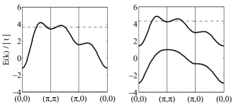
Figure 1: Band picture of the $t-V$–model without account for the SICs (left) and with account for the SICs (right) for the set of parameters $t^{\prime}=-0.1,\,t^{\prime\prime}=-0.5,\,V=2.5$ (in terms of $|t|$) and holes concentration $h=0.15$. Dashed lines show the chemical potential.

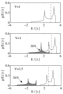
Figure 2: Density of states of the $t-V$–model calculated for $h=0.25$ without account for the SICs $V=1$ (top), with account for the SICs at $V=1$ (middle) an at $V=2.5$ (bottom). Here $t^{\prime}=-0.1,\,t^{\prime\prime}=-0.5$ (all in terms of $|t|$). Dashed lines show the chemical potential.

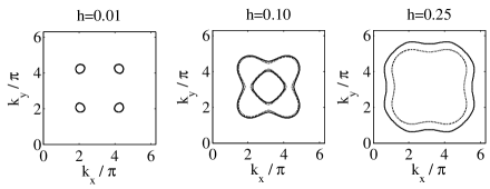
Figure 3: Fermi surfaces calculated for the set of parameters $t^{\prime}=-0.1,\,t^{\prime\prime}=-0.5,\,V=2.5$ ( in terns of $|t|$) and different $h$ without account for the SICs (dashed lines) and with account for the SICs (solid lines).

The occurrence of the BFS qualitatively changes the electron density of states of the Hubbard fermions. The upper graph in Fig.2 shows the density of states of the $t-V$–model with disregard of the SICs. It is seen that ignoring these correlations leads to trivial displacement of the band position.

The energy dependence of the sum electron density of states of the $t-V$–model for the same set of parameters, but with regard of the SICs, is shown by a bold solid line in the middle graph of Fig.2. Comparison with the upper graph evidences that the account for the SICs yields noticeable qualitative changes in the density of states: the latter acquires a three-peak structure instead of the two-peak one. The occurrence of the additional peak corresponds to the formation of the BFS. For clarity, BFS density $g^{-}(E)$ is reflected in the graph by the line which bounds the shaded area. The BFS fraction is 36% of the whole number of states of the system, whereas the fraction of the ground band with density of states $g^{+}(E)$ is 64%. Summation of densities $g^{+}(E)$ and $g^{-}(E)$ gives total density $g(E)$ with the three peaks.

More substantial changes in the energy structure of the $t-V$–model take place at high values of the intersite Coulomb interaction. It is seen from the lower graph in Fig.2 which presents the same dependences as in the two upper graphs but calculated for $V=2.5$ (the rest parameters are not changed). In this case, the SICs lead to splitting the BFS off and the formation of a gap in the energy spectrum. The graphs presented in Fig.2 are calculated at $h=0.25$. In the case of $h=0$ the SIC contribution becomes zero and the density of states of the system will be such as shown in the upper graph in Fig.2. This suggests the presence of a qualitatively new effect related to the account for the SIC: upon doping not only the chemical potential shifts but the density of states rearranges.

The growth of the BFS spectral intensity with an increase in doping level leads to renormalization of the dependence of the chemical potential on hole concentration in the system. As a result in the area of optimal doping $h\simeq 0.2$ the square bounded by the Fermi contour noticeably grows. The Fermi contour calculated at $h=0.25$ with disregard of the SICs is shown by dotted lines in Fig.3. If the correlations are taken into account then the Fermi contour noticeably grows and acquires the form shown by solid lines. In this case the change in the square bounded by the Fermi contour reaches $16\%$ (right graph). This increase is important for description of the Lifshitz quantum phase transitions occurring upon doping SGO and for interpretation of the experimental data on measuring magnetic oscillations in the de Haas–van Alphen effect. Recently, such measurements have been performed by many researchers due to substantial improvement of quality of materials and novel techniques with the use of the strong magnetic fields.

Note in summary that the hybridization character of the energy spectrum with regard of the SICs is related to the fact that electron hoppings between the nearest neighbors lead to the transitions between the one-site energy levels which differ by $V$. Therefore, the intensity of such hybridization processes is proportional to both hopping parameter $t$ and the above-mentioned mean-square fluctuation of the occupation numbers. Note also that the considered modification of the energy structure due to the SICs is general and not limited merely by the $t-V$–model. One should expect that the effects discovered in this study will be especially important for the systems with variable valence.

This study was supported by the program ”Quantum physics of condensed matter” of the Presidium of the Russian Academy of Sciences (RAS); the Russian Foundation for Basic Research (project No. 07-02-00226); the Siberian Division of RAS (Interdisciplinary Integration project No. 53). One of authors (M.K.) would like to acknowledge the support of the Dynasty Foundation.

References

- (1) J. C. Hubbard, Proc. R. Soc. London A 276, 238 (1963).
- (2) P. W. Anderson, Science 235, 1196 (1987).
- (3) R. O. Zaitsev, Zhur. Eksp. Teor. Fiz. 78, 1132 (1980).
- (4) R. O. Zaitsev, JETP 98, 780 (2004).
- (5) L. M. Falicov and J. C. Kimball, Phys. Rev. Lett. 22, 997 (1969).
- (6) D. I. Khomskii, Sov. Phys. Usp. 22, 879 (1979).
- (7) H. Matsukawa and H. Fukuyama, J. Phys. Soc. Japan 58, 2845 (1989).
- (8) P. B. Littlewood, C. M. Varma, and E. Abrahams, Phys. Rev. Lett. 63, 2602 (1989).
- (9) A. J. Fedro and H.-B. Schüttler, Phys. Rev. B 40, 5155 (1989).
- (10) M.-R. Li, Y.-J. Wang, and C.-D. Gong, Phys. Rev. B 46, 3668 (1992).
- (11) D. M. Larsen, Phys. Rev. B 53, 15719 (1996).
- (12) Y. Onishi and K. Miyake, J. Phys. Soc. Japan 69, 3955 (2000).
- (13) R. Neudert et al., Phys. Rev. B 62, 10752 (2000).
- (14) C. Barreteau et al., Phys. Rev. B 69, 064432 (2004).
- (15) K. Miyake, J. Phys.: Condens. Matter 19, 1 (2007).
- (16) V. V. Val’kov and M. M. Korovushkin, Eur. Phys. J. B 69, 219 (2009).
- (17) J. C. Hubbard, Proc. R. Soc. London A 285, 542 (1965).
- (18) S. G. Ovchinnikov and V. V. Val’kov, Hubbard Operators in the Theory of Strongly Correlated Electrons (Imperial College Press, London, 2004).
- (19) R. Zwanzig, Phys. Rev. 124, 983 (1961).
- (20) H. Mori, Prog. Theor. Phys. 33, 423 (1965).
- (21) S. G. Ovchinnikov, M. M. Korshunov, and E. I. Shneyder, Zhur. Eksp. Teor. Fiz. 136, 898 (2009); arXiv:0909.2308v1.