Computation of geometric measure of entanglement for pure multiqubit states

Abstract

We provide methods for computing the geometric measure of entanglement for two families of pure states with both experimental and theoretical interests: symmetric multiqubit states with non-negative amplitudes in the Dicke basis and symmetric three-qubit states. In addition, we study the geometric measure of pure three-qubit states systematically in virtue of a canonical form of their two-qubit reduced states, and derive analytical formulae for a three-parameter family of three-qubit states. Based on this result, we further show that the W state is the maximally entangled three-qubit state with respect to the geometric measure.

I Introduction

Quantum entanglement, which was first noted by Einstein and Schrödinger schrodinger35 ; epr35 , has been extensively studied in the past 20 years hhh09 . In particular, multipartite entanglement has attracted increasing attention due to its intriguing properties and potential applications in quantum information processing.

The importance of multipartite entanglement can be illustrated in two aspects. In respect of application, graph states, prominent examples of entangled multiqubit states, are a useful resource for one-way quantum computation rb01 and fault-tolerant topological quantum computation lgg09 . Multipartite entangled states, such as GHZ states, are essential resources for quantum secret sharing hbb99 ; spc09 . In addition, multipartite entangled states can serve as multiparty quantum channels in virtue of teleportation bbc93 . In respect of theoretical interests, multipartite states display stronger nonlocality, one of the key features of quantum physics ghz89 ; ghsz90 ; bbg09 . Quantum cryptography beyond pure entanglement distillation has been generalized to multipartite bound entangled states ah09 . What’s more, recent progress in experiments has made accessible more multipartite entangled states, such as the GHZ states lzg07 , W states pcd09 , six-photon Dicke states dicke54 ; wkk09 ; pct09 etc. Methods for detecting such states have also been developed kkb09 .

Given an entangled state, a natural question to ask is how much entanglement is contained in this state. In quantum information theory, entanglement is usually quantified by entanglement measures vidal00 . An entanglement measure is an entanglement monotone, which cannot increase under local operations and classical communications (LOCC), and equal to zero for only classically correlated (separable) states bds96 . Hitherto, the most well-known entanglement measures are defined for bipartite states, such as entanglement cost and distillable entanglement bds96 ; pv07 . For pure bipartite states, there is essentially a unique entanglement measure, the von Neumann entropy of each reduced density matrix, which is easily computable nc00 .

For multipartite states, while a lot of entanglement measures have been proposed hhh09 ; mw02 ; wg03 ; bh01 , the characterization of multipartite entanglement is far from being complete. It is generally difficult to calculate such measures even numerically. Moreover, the existence of many types of inequivalent entanglement defies a unique definition. Different entanglement measures often induce different orders and even lead to different maximally entangled states. For example, the Bell state $|\Psi\rangle=\frac{1}{\sqrt{2}}(|00\rangle+|11\rangle)$ is the maximally entangled state of a two-qubit system for all measures, since it violates the Bell inequality most strongly. However, its multipartite analog, the GHZ state $|\mathrm{GHZ}\rangle=\frac{1}{\sqrt{2}}(|000\rangle+|111\rangle)$, is maximally entangled only under some specific entanglement measures, such as three-tangle ckw00 ; twp09 . It is also maximally entangled under any bipartition of systems ffp08 . Nevertheless, the GHZ state consisting of more than three qubits is not a maximally entangled state under the definition in ffp08 , and the geometric measure of entanglement. This is one focus of the present paper.

On the other hand, some geometrically motivated multipartite entanglement measures have been providing us insights on quantum entanglement. One prominent example is the geometric measure of entanglement (GM), bh01 ; wg03 which quantifies the minimum distance between a given state and the set of product states. In addition to providing a simple geometric picture, GM has significant operational meanings. It is closely related to optimal entanglement witnesses wg03 ; hmm08 , and has been shown to quantify the difficulty of multipartite state discrimination under LOCC hmm06 . Recently, GM has also been applied to show that most entangled states are too entangled to be useful as computational resources gfe09 . In condensed matter physics, GM has been utilized to study the ground state properties and to characterize quantum phase transitions oru08 ; odv08 ; oru08b ; ow09 .

There have been extensive literatures on the quantitative calculation of GM for both pure and mixed states wg03 ; hmm08 ; hs09 ; tpt08 ; tkk09 ; pr09 ; chen09 . The qualitative analysis on GM has also received much attention mmm09 ; hkw09 . In addition, a few numerical methods have been developed for computing the GM of multipartite states, such as the algorithms presented in Refs. sb07 ; msb10 , which allow repeated analytical maximization according to a subset of the parameters with a high efficiency. However, our knowledge about GM is still quite limited. Even for pure three-qubit states, there is no complete analytical solution. In addition, it is still uncertain which state is the maximally entangled with respect to GM, although the authors of twp09 conjectured that the W state is such a candidate. Thus it is desirable to compute GM analytically for more entangled states, which is another focus of the present paper.

In this paper, we would like to compute the GM for several families of multipartite pure states and determine the maximally entangled three-qubit states with respect to GM. Throughout the paper, by symmetric states, we mean those states which are supported on the symmetric subspace of the whole Hilbert space.

First, we present an analytical method for computing the GM of symmetric multiqubit states composed of Dicke states with non-negative amplitudes by virtue of a recent simplification on GM of symmetric states hkw09 . Next, we analytically compute the GM for symmetric three-qubit states. Combining with the results in Ref. tkk09 , we provide a complete analytical solution to GM of any symmetric pure three-qubit states. Recall that many important multiqubit states accessible to experiments so far are symmetric, e.g. GHZ states lzg07 , W states pcd09 , and Dicke states wkk09 ; pct09 etc. Our results may hopefully help analyze these states in experiments.

Second, we introduce a canonical form of pure three-qubit states based on the canonical form of two-qubit rank-two states developed in Ref. em02 . In virtue of this canonical form, we study the GM of pure three-qubit states systematically and derive explicit analytical formulae of GM for a three-parameter family of three-qubit states. Starting from these results, we prove that, up to local unitary transformations, the W state is the unique maximally entangled pure three-qubit state with respect to GM, confirming the conjecture made in Ref. twp09 .

The rest of the paper is organized as follows. In Sec. II, we propose analytical methods for computing the GM of symmetric multiqubit states with non-negative amplitudes and that of symmetric three-qubit states. In Sec. III, we derive analytical formulae of GM for a three-parameter family of pure three-qubit states and prove that the W state is the maximally entangled state under GM. We conclude in Sec. IV.

II Analytical method for computing geometric measure (I): symmetric states

The definition of GM of bipartite or multipartite pure states is motivated by the following simple geometric idea of entanglement quantification: the farther away from the set of separable states, the more entangled a state is wg03 . Given a pure state $|\psi\rangle$ of a joint system composed of subsystems $A,B,C,\cdots$, define $G(|\psi\rangle)$ as the maximum overlap between $|\psi\rangle$ and the set of product states, that is,

$$G(|\psi\rangle):=\underset{|\varphi\rangle=|a\rangle|b\rangle|c\rangle\ldots}{\mathrm{max}}\big{|}\langle\varphi|\psi\rangle\big{|},$$ (1)

where the normalized one-particle states $|a\rangle,|b\rangle,|c\rangle,\cdots$ belong to subsystems $A,B,C,\ldots$, respectively. $G(|\psi\rangle)$ is manifestly invariant under local unitary transformations. It obtains the maximum value 1 only for product states and is thus an inverted entanglement measure. The GM of a pure state is defined as follows:

$$E_{G}(|\psi\rangle):=1-G(|\psi\rangle)^{2},$$ (2)

or in another version $-2~{}\text{log}\ G(|\psi\rangle)$ sometimes. In this paper we will follow the definition in Eq. (2). It can be extended to the GM of mixed states by convex roof construction wg03 according to the same idea as in the definition of entanglement of formation bds96 :

$$E_{G}(\rho):=\underset{\rho=\sum_{i}p_{i}|\psi_{i}\rangle\!\langle\psi_{i}|}{\mathrm{min}}\sum_{i}p_{i}E_{G}(|\psi_{i}\rangle).$$ (3)

$E_{G}(\rho)$ has been shown to be an entanglement monotone by T.-C. Wei and P. M. Goldbart wg03 . An alternative definition of GM for mixed states will be introduced in Sec. III in a different context.

Clearly, $E_{G}(|\psi\rangle)$ in Eq. (2) is determined by $G(|\psi\rangle)$ in Eq. (1). From now on we focus on $G(|\psi\rangle)$ of pure states $|\psi\rangle$ and call it GM too, if there is no confusion. For a pure bipartite state, the GM is equal to its largest Schmidt coefficient. The problem becomes difficult for pure multipartite states, since there is no Schmidt decomposition in general. The difficulty lies in the linearly increasing number of optimization variables parametrizing the product states $|a\rangle|b\rangle|c\rangle\cdots$ in Eq. (1), as the number of parties increases. In fact, only a few partial results are available on this problem tpt08 ; wg03 ; tkk09 ; twp09 .

Recently, the authors of Ref. hkw09 proved that, for a symmetric pure state $|\psi^{\mathrm{sy}}\rangle$, it suffices to consider symmetric product states in the maximization in Eq. (1), that is,

$$G(|\psi^{\mathrm{sy}}\rangle)=\underset{|\varphi\rangle=|a\rangle|a\rangle|a\rangle\ldots}{\mathrm{max}}\big{|}\langle\varphi|\psi^{\mathrm{sy}}\rangle\big{|}.$$ (4)

This result can greatly simplify the calculation of GM for symmetric states. In the rest of this section, we derive analytical solutions for two families of states, respectively, in virtue of this result. In Sec. II.1, we analytically derive GM for symmetric multiqubit states with non-negative amplitudes in the Dicke basis. In Sec. II.2, we derive the analytical solution of GM for symmetric pure three-qubit states based on the previous work tkk09 , thus solving this problem completely.

II.1 symmetric multiqubit states with non-negative amplitudes

In this subsection, we compute the GM for pure symmetric multiqubit states with non-negative amplitudes in the Dicke basis. More explicitly, we investigate the $N$-qubit state

$$|\psi^{\mathrm{symq}}\rangle:=\sum^{N}_{m=0}a_{m}|m,N\rangle,$$ (5)

where $a_{m}\geq 0$, and $|m,N\rangle$ is the Dicke state dicke54 defined as

$$|m,N\rangle:={N\choose m}^{-1/2}\sum_{k}P_{k}|\overbrace{1,...,1}^{m},\overbrace{0,...,0}^{N-m}\rangle,$$ (6)

where $P_{k}$s denote the set of all permutations of the spins. By definition, Dicke states are symmetric; so the state $|\psi^{\mathrm{symq}}\rangle$ is also symmetric, and we can apply Eq. (4) to computing its GM. Let $|a\rangle=\cos\alpha|0\rangle+e^{i\theta}\sin\alpha|1\rangle$ with $\alpha\in[0,\frac{\pi}{2}]$ and $\theta\in[0,2\pi]$; then the GM of the state in Eq. (5) reads

$$G(|\psi^{\mathrm{symq}}\rangle)$$

$$=\underset{|\varphi\rangle=|a\rangle|a\rangle|a\rangle\ldots}{\mathrm{max}}\bigg{|}\sum^{N}_{m=0}{N\choose m}^{1/2}a_{m}\cos^{N-m}\alpha\sin^{m}\alpha e^{-im\theta}\bigg{|},$$

$$\leq\underset{|\varphi\rangle=|a\rangle|a\rangle|a\rangle\ldots}{\mathrm{max}}\sum^{N}_{m=0}\bigg{|}{N\choose m}^{1/2}a_{m}\cos^{N-m}\alpha\sin^{m}\alpha\bigg{|},$$

$$=\underset{\alpha\in[0,\frac{\pi}{2}]}{\mathrm{max}}\sum^{N}_{m=0}{N\choose m}^{1/2}a_{m}\cos^{N-m}\alpha\sin^{m}\alpha,$$ (7)

where the equality holds when $\theta=0$. Equation (II.1) contains only one variable $\alpha$, so one can easily find out the maximum. For example, let $x=\tan\alpha$, then one can convert $G^{2}(|\psi^{\mathrm{symq}}\rangle)$ into a rational fraction ${A(x)}/{B(x)}$, where $A(x)$ and $B(x)$ are both polynomials on $x$. By calculating its derivative we can find out the maximum in Eq. (II.1) explicitly.

A similar idea can be applied to calculating the GM of any symmetric multi-qudit state with nonnegative amplitudes in the generalized Dicke basis; again the number of free variables can be reduced by half. Recently, the additivity of GM of states with non-negative amplitudes was proved, i.e., $G(|\alpha\rangle\otimes|\beta\rangle)=G(|\alpha\rangle)~{}G(|\beta\rangle)$  zch10 . So we can compute the GM of $|\psi^{\mathrm{symq}}\rangle\otimes|\beta\rangle$ if we know the GM of $|\beta\rangle$ too.

Unfortunately, the present method does not apply to arbitrary symmetric multiqubit states, e.g., those states in Eq. (5) having negative or complex amplitudes. For more complicated states, numerical methods are indispensable for computing their entanglement measures, see, for example, Refs. sb07 ; msb10 .

II.2 symmetric three-qubit states

In this subsection, we compute the GM of symmetric pure three-qubit states. Such states can always be converted into the following form with suitable local unitary operations tkk09 :

$$|\Phi\rangle=g|000\rangle+t(|011\rangle+|101\rangle+|110\rangle)+e^{i\gamma}h|111\rangle,$$ (8)

where $g,t,h\geq 0$ and $\gamma\in[-\frac{\pi}{2},\frac{\pi}{2}]$. So it suffices to calculate the GM for the state $|\Phi\rangle$.

Analytical formula of the GM is already known if at least one of the three parameters $g,t,h$ is vanishing, or $\gamma=0,\pm\frac{\pi}{2}$ wg03 ; tpt08 ; hmm08 ; tkk09 ; notation1 . Hence, we can focus on the family of states with

$$g,t,h>0,\;\;g^{2}+3t^{2}+h^{2}=1,\;\;\gamma\in(-\frac{\pi}{2},0)\cup(0,\frac{\pi}{2}).$$

The authors of Ref. tpt08 have reduced the task of computing the GM of the state $|\Phi\rangle$ to solving the following system of equations of the three variables $\varphi,\theta,\lambda$ (see also appendix A):

$$2ht\cos\gamma+2t(g+t)\sin\theta\cos\varphi-$$

$$2ht\cos\gamma\cos\theta= \lambda\sin\theta\cos\varphi,$$ (10)

$$2ht\sin\gamma-2t(g-t)\sin\theta\sin\varphi-$$

$$2ht\sin\gamma\cos\theta= \lambda\sin\theta\sin\varphi,$$ (11)

$$(g^{2}-t^{2})(1+\cos\theta)-h^{2}(1-\cos\theta)-$$

$$2ht\cos\gamma\sin\theta\cos\varphi-2ht\sin\gamma\sin\theta\sin\varphi= \lambda\cos\theta.$$ (12)

For each root $(\varphi_{j},\theta_{j})$ of Eqs. (II.2)–(II.2), we can obtain a GM candidate of the state $|\Phi\rangle$ via the following formula, according to Eq. (Appendix A: Derivation of Eqs. (–)) in appendix A,

$$G_{j}^{2}(|\Phi\rangle) =\frac{1}{8}\big{[}3-2t^{2}+4(1-2h^{2}-4t^{2})\cos\theta_{j}$$

$$+(1-6t^{2})\cos 2\theta_{j}+4gt\cos 2\varphi_{j}\sin^{2}\theta_{j}$$

$$+32ht\cos(\gamma-\varphi_{j})\cos\frac{\theta_{j}}{2}\sin^{3}\frac{\theta_{j}}{2}\big{]};$$ (13)

the GM is the maximum over all the GM candidates:

$$G^{2}(|\Phi\rangle)=\underset{j}{\mathrm{max}}\,G_{j}^{2}(|\Phi\rangle).$$ (14)

We shall solve Eqs. (II.2)–(II.2) in two cases separately; the second case consists of three subcases. In each case we obtain one or a few GM candidates by computing Eq. (II.2) with the solutions to the system of equations.

Case 1. Suppose $\theta=0$; then the phase $\varphi$ does not play any role, and Eqs. (II.2) and (II.2) become identities, while Eq. (II.2) determines $\lambda$. In this case we get a GM candidate via Eq. (II.2) as follows:

$$G_{1}^{2}(|\Phi\rangle)=g^{2}.$$ (15)

Case 2 To satisfy Eqs. (II.2)–(II.2), the roots $\varphi=k\frac{\pi}{2}$ for $k=0,1,2,3$ lead to $\theta=0$, which is already discussed. Moreover, $\theta=\pi$ cannot be a legal solution of Eqs. (II.2) or (II.2), so this choice is excluded. Hence, it remains to solve Eqs. (II.2)–(II.2) under the assumption that

$$\varphi \in(0,\frac{\pi}{2})\cup(\frac{\pi}{2},\pi)\cup(\pi,3\frac{\pi}{2})\cup(3\frac{\pi}{2},2\pi),\quad\theta\in(0,\pi).$$ (16)

From Eqs. (II.2–II.2), we can determine $\lambda$ as a function of $\theta$ and $\varphi$. Inserting this solution into Eq. (II.2) and Eq. (II.2), we can obtain two equations about $\theta$ and $\varphi$: $\text{eq}1(\varphi,\theta)=0$ and $\text{eq}2(\varphi,\theta)=0$, respectively. This further implies that either

$$\tan\frac{\theta}{2}=\frac{g}{h\csc 2\varphi\sin(\gamma-\varphi)},$$ (17)

or

$$\tan\frac{\theta}{2}=\frac{-t}{h\csc 2\varphi\sin(\gamma+\varphi)}.$$ (18)

Combining either of them and $\text{eq}1(\varphi,\theta)=0$ can lead to a set of solutions.

Case 2.1 There is a simple solution $\tan\varphi=\frac{t+g}{t-g}\tan{\gamma}$. The variable $\theta$ can be determined via either Eq. (17) or (18), which lead to an identical result in this case. Inserting this solution into Eq. (II.2), we get another GM candidate:

$$G_{2}^{2}(|\Phi\rangle)=g^{2}-\frac{(g^{2}-t^{2})^{3}}{t^{2}-2t^{4}+g^{2}-6g^{2}t^{2}-2gth^{2}\cos 2\gamma}.$$ (19)

Case 2.2 By combining Eq. (17) and $\text{eq}1(\varphi,\theta)=0$, we can get two polynomial equations:

$$\sum^{4}_{i=0}c_{1i}(g,t,h,\gamma)\cos^{i}2\varphi=0,$$

$$\sum^{4}_{i=0}c_{2i}(g,t,h,\gamma)\cos^{i}2\varphi=0,$$ (20)

as well as Case 2.1, which has already been handled. Since Eqs. (II.2) are quartic equations on $\cos 2\varphi$, we can analytically derive their roots. We may obtain up to 16 different phases $\varphi\in[0,2\pi]$. The variable $\theta$ can then be determined via Eq. (17). Hence, we can derive up to 16 GM candidates $G_{j}(|\Phi\rangle)$ for $j=3,\ldots,18$ via Eq. (II.2). This differs a bit from Case 1 and Case 2.1, where only one GM candidate is given respectively.

Case 2.3 Similar to Case 2.2, by combining Eq. (18) and $\text{eq}1(\varphi,\theta)=0$, we can get two quartic polynomial equations on $\cos 2\varphi$, which are analytically solvable. Again we may get up to 16 GM candidates $G_{j}(|\Phi\rangle)$ for $j=19,\ldots,34$. This finishes the discussion of Case 2.

Now we have all the GM candidates $G_{j}(|\Phi\rangle)$ for $j=1,\ldots,34$. The maximum of them is exactly the GM of the state $|\Phi\rangle$ in Eq. (8).

For the convenience of the readers, here we repeat the main steps for deriving the GM of the symmetric three-qubit state $|\Phi\rangle$.

Step 1. Compute $G_{1}(|\Phi\rangle)$ and $G_{2}(|\Phi\rangle)$ via Eqs. (15) and  (19), respectively; two GM candidates can be obtained.

Step 2. Compute $G_{j}(|\Phi\rangle)$ for $j=3,\ldots,18$ via Eq. (II.2) with roots ($\varphi_{j},\theta_{j}$) of Eqs. (17) and  (II.2); up to 16 GM candidates can be obtained.

Step 3. Similar to Step 2, with the roots ($\varphi_{j},\theta_{j}$) for $j=19,\ldots,34$ of Eq. (18) and quartic equations similar to Eq. (II.2), up to 16 GM candidates can be obtained via Eq. (II.2).

Step 4. The maximum of all 34 GM candidates is exactly the GM of the state $|\Phi\rangle$.

In conclusion, we have provided a method for analytically deriving the GM of the symmetric three-qubit states in Eq. (8) with $\gamma\in(-\frac{\pi}{2},0)\cup(0,\frac{\pi}{2})$. The special cases $\gamma=0,\pm\frac{\pi}{2}$ have been addressed in Ref. tkk09 . Calculation shows that our result approaches their result when $\gamma$ approaches these special values. Hence, we can now compute the GM of any symmetric pure three-qubit states.

III Analytical method for computing geometric measure (II): maximal entangled states among pure three-qubit states

In this section, we introduce a canonical form of pure three-qubit states based on the canonical form of two-qubit rank-two states developed in Ref. em02 . By virtue of this canonical form, the GM of pure three-qubit states is studied systematically. In particular, we derive analytical formulae of GM for the family of pure three-qubit states one of whose rank-two two-qubit reduced states is the convex combination of the maximally entangled state and its orthogonal pure state within the rank-two subspace. Based on these results, we prove that the W state is the maximally entangled three-qubit state with respect to GM, confirming the conjecture in Ref. twp09 .

Our approach builds on Theorem 1 in Ref. jung08 , which states that the GM of an $n$-partite pure state $|\psi\rangle$ is determined by any of its ($n-1$)-partite reduced states $\rho$, that is,

$$G^{2}(|\psi\rangle)=g(\rho).$$

Here $g(\rho)$ is an alternative definition of geometric measure and has nothing to do with the parameter $g$ introduced in Eq. (8):

$$g(\rho)=\underset{\rho_{1},\ldots,\rho_{n-1}}{\operatorname{max}}\;\mathrm{tr}\bigl{[}\rho(\rho_{1}\otimes\cdots\otimes\rho_{n-1})\bigr{]},$$ (21)

where $\rho_{1},\ldots,\rho_{n-1}$ are pure single-particle states, namely $\rho_{i}=|a_{i}\rangle\!\langle a_{i}|$. In addition, to any closest product state $\rho_{1}\otimes\cdots\otimes\rho_{n-1}$ of $\rho$, there corresponds a unique closest product state of $|\psi\rangle$ with $\rho_{1}\otimes\cdots\otimes\rho_{n-1}$ as a reduced state. A closest product state of $\rho$ is any pure product state $\rho_{1}\otimes\cdots\otimes\rho_{n-1}$ that maximizes Eq. (21). From the definition, $g(\rho)$ is a convex function of $\rho$; this property will be frequently resorted to later.

Note that for a mixed state $\rho$, $g(\rho)$ is not the standard definition of the GM of $\rho$ (see the first paragraph of Sec. II). Nevertheless, this alternative definition is useful for computing the GM of any purification of $\rho$ jung08 . It has also many applications of its own, such as constructing optimal entanglement witnesses wg03 ; hmm08 and quantifying the difficulty of state discrimination under LOCC hmm06 ; hmm08 .

III.1 Canonical form of two-qubit rank-two states

In this section we introduce a canonical form of pure three-qubit states based on the canonical form of two-qubit rank-two states developed in Ref. em02 and set the notations useful in later discussions.

For a pure three-qubit state, each two-qubit reduced state lies on a rank-two subspace of the two-qubit Hilbert space. Up to local unitary transformations, the projector $\Sigma_{0}$ onto a general rank-two subspace can be specified by just two parameters $\gamma_{1},\gamma_{2}$ em02 :

$$\Sigma_{0} = \frac{1}{2}(1+u\sigma_{3}+v\tau_{3}+z_{1}\sigma_{1}\tau_{1}+z_{2}\sigma_{2}\tau_{2}),$$

$$u = \cos\gamma_{1}\cos\gamma_{2},~{}~{}v=\sin\gamma_{1}\sin\gamma_{2},$$

$$z_{1} = \sin\gamma_{1}\cos\gamma_{2},~{}~{}z_{2}=\cos\gamma_{1}\sin\gamma_{2},$$ (22)

$$\mbox{with}\quad\frac{1}{2}\pi\geq\gamma_{1}\geq\gamma_{2}\geq 0,$$

where $\sigma_{1},\sigma_{2},\sigma_{3}$ are the Pauli operators for the first qubit and $\tau_{1},\tau_{2},\tau_{3}$ are that for the second qubit. Interchange of the two qubits leads to $\gamma_{1}\rightarrow\frac{\pi}{2}-\gamma_{2}$, $\gamma_{2}\rightarrow\frac{\pi}{2}-\gamma_{1}$. So without loss of generality, we can assume $\gamma_{1}+\gamma_{2}\leq\frac{\pi}{2}$, $\gamma_{2}\leq\frac{\pi}{4}$.

Any rank-two state supported on $\Sigma_{0}$ can be written as follows:

$$\rho_{\mathrm{rk}2} = \frac{1}{2}(\Sigma_{0}+x_{1}\Sigma_{1}+x_{2}\Sigma_{2}+x_{3}\Sigma_{3}),$$ (23)

where $\Sigma_{1},\Sigma_{2},\Sigma_{3}$ are the Pauli operators for the rank-two subspace em02 :

$$\Sigma_{1} = \frac{1}{2}(\sin\gamma_{1}\sigma_{1}+\cos\gamma_{2}\tau_{1}+\sin\gamma_{2}\sigma_{1}\tau_{3}+\cos\gamma_{1}\sigma_{3}\tau_{1}),$$

$$\Sigma_{2} = \frac{1}{2}(\sin\gamma_{2}\sigma_{2}+\cos\gamma_{1}\tau_{2}+\sin\gamma_{1}\sigma_{2}\tau_{3}+\cos\gamma_{2}\sigma_{3}\tau_{2}),$$

$$\Sigma_{3} = \frac{1}{2}(v\sigma_{3}+u\tau_{3}-z_{2}\sigma_{1}\tau_{1}-z_{1}\sigma_{2}\tau_{2}+\sigma_{3}\tau_{3}),$$ (24)

and $(x_{1},x_{2},x_{3})$ (satisfying $x_{1}^{2}+x_{2}^{2}+x_{3}^{2}\leq 1$) is the Bloch vector of $\rho_{\mathrm{rk}2}$.

Local unitary symmetry and complex conjugation symmetry play an important role in determining the behavior of $g(\rho_{\mathrm{rk}2})$ and in simplifying its calculation. According to Eqs. (III.1) and (III.1), simultaneous local unitary transformation $\sigma_{3}\otimes\tau_{3}$ flips the sign of $\Sigma_{1},\Sigma_{2}$, while leaving $\Sigma_{0},\Sigma_{3}$ invariant, that is,

$$\sigma_{3}\otimes\tau_{3}\Sigma_{0,3}\sigma_{3}\otimes\tau_{3} = \Sigma_{0,3},$$

$$\sigma_{3}\otimes\tau_{3}\Sigma_{1,2}\sigma_{3}\otimes\tau_{3} = -\Sigma_{1,2};$$ (25)

under this transformation, the Bloch vector of $\rho_{\mathrm{rk}2}$ changes as follows: $(x_{1},x_{2},x_{3})\rightarrow(-x_{1},-x_{2},x_{3})$. Complex conjugation flips the sign of $\Sigma_{2}$, that is

$$\Sigma_{j}^{*}=(-1)^{\delta_{j,2}}\Sigma_{j},$$ (26)

where $\delta_{j,2}$ is the Kronecker $\delta$ function; under this transformation, the Bloch vector of $\rho_{\mathrm{rk}2}$ changes as follows: $(x_{1},x_{2},x_{3})\rightarrow(x_{1},-x_{2},x_{3})$ . As a consequence of these symmetries, any reasonable entanglement measure is equal for the four states $\rho_{\mathrm{rk}2}$ with Bloch vectors $(\pm x_{1},\pm x_{2},x_{3})$, respectively. Without loss of generality, we can assume $x_{1},x_{2}\geq 0$.

If $\gamma_{1}=\gamma_{2}$, the simultaneous local unitary transformation $\mathrm{e}^{-\mathrm{i}\theta\sigma_{3}\otimes\tau_{3}}$ rotates the Bloch vector of $\rho_{\mathrm{rk}2}$ around the $x_{3}$ axis, so $g(\rho_{\mathrm{rk}2})$ is rotationally invariant about the $x_{3}$ axis. If $\gamma_{2}=0$, the local unitary transformation $\mathrm{e}^{-\mathrm{i}\theta\tau_{1}}$ rotates the Bloch vector around the $x_{1}$ axis, so $g(\rho_{\mathrm{rk}2})$ is rotationally invariant about the $x_{1}$ axis.

Up to local unitary transformations, there is a one-to-one correspondence between pure three-qubit states and rank-two two-qubit states. Hence, the canonical form of rank-two two-qubit states provides a canonical form of pure three-qubit states. Moreover, due to Theorem 1 in Ref. jung08 and the arguments given above, computing the GM of pure three-qubit states can be reduced to computing $g(\rho_{\mathrm{rk}2})$ of the family of canonical rank-two two-qubit states in Eq. (23) with $0\leq\gamma_{2}\leq\gamma_{1}\leq\frac{\pi}{2}$, $\gamma_{2}+\gamma_{1}\leq\frac{\pi}{2}$, $0\leq x_{1},x_{2}\leq 1$ and $-1\leq x_{3}\leq 1$. With this background, we can now study the GM of pure three-qubit states systematically.

III.2 $g(\rho_{\mathrm{rk}2})$ of general two-qubit rank-two states

In this subsection we reduce the task of computing $g(\rho_{\mathrm{rk}2})$ for general two-qubit rank-two states to a maximization problem which involves only two free variables. The number of free variables is further reduced to one for states $\rho_{\mathrm{rk}2}$ with $x_{2}=0$.

Let $\rho_{1}=\frac{1}{2}(1+\bm{s}_{1}\cdot\bm{\sigma})$ and $\rho_{2}=\frac{1}{2}(1+\bm{s}_{2}\cdot\bm{\tau})$ be two pure qubit states with Bloch vectors $\bm{s}_{1}=(a,b,c)$ and $\bm{s}_{2}=(a_{2},b_{2},c_{2})$, respectively. Straightforward calculation shows that

$$\mathrm{tr}(\rho_{\mathrm{rk}2}\rho_{1}\otimes\rho_{2})=\frac{1}{4}(1+ax_{1}\sin\gamma_{1}+bx_{2}\sin\gamma_{2}$$

$${}+c\cos\gamma_{1}\cos\gamma_{2}+cx_{3}\sin\gamma_{1}\sin\gamma_{2}+\bm{w}\cdot\bm{s}_{2}),$$ (27)

where

$$\bm{w} =\left(\begin{array}[]{c}a(\cos\gamma_{2}\sin\gamma_{1}-x_{3}\cos\gamma_{1}\sin\gamma_{2})\\ b(-x_{3}\cos\gamma_{2}\sin\gamma_{1}+\cos\gamma_{1}\sin\gamma_{2})\\ bx_{2}\sin\gamma_{1}+ax_{1}\sin\gamma_{2}\\ \end{array}\right)^{T}$$ (35)

$${}+\left(\begin{array}[]{c}cx_{1}\cos\gamma_{1}+x_{1}\cos\gamma_{2}\\ x_{2}\cos\gamma_{1}+cx_{2}\cos\gamma_{2}\\ cx_{3}+x_{3}\cos\gamma_{1}\cos\gamma_{2}+\sin\gamma_{1}\sin\gamma_{2}\\ \end{array}\right)^{T}.$$

Given $\rho_{\mathrm{rk}2}$ and $\rho_{1}$, the trace in Eq. (27) is maximized when $\bm{s}_{2}$ is parallel to $\bm{w}$. According to Eq. (21), we have

$$g(\rho_{\mathrm{rk}2}) =\underset{\rho_{1}\rho_{2}}{\operatorname{max}}\;\mathrm{tr}(\rho_{\mathrm{rk}2}\rho_{1}\otimes\rho_{2})$$

$$=\frac{1}{4}\underset{a^{2}+b^{2}+c^{2}=1}{\operatorname{max}}f(a,b,c),$$

$$f(a,b,c) =(1+ax_{1}\sin\gamma_{1}+bx_{2}\sin\gamma_{2}+c\cos\gamma_{1}\cos\gamma_{2}$$ (36)

$$\quad{}+cx_{3}\sin\gamma_{1}\sin\gamma_{2}+|\bm{w}|),$$

where $|\bm{w}|$ denotes the Euclidian norm of $\bm{w}$. Thus we have reduced the task of computing $g(\rho_{\mathrm{rk}2})$ to that of maximizing the function $f(a,b,c)$ on the unit sphere determined by $a^{2}+b^{2}+c^{2}=1$, which involves only two free variables. The contours of $f$ are in general some quadratic surfaces. At the maximum of $f$ over the unit sphere, the contour is generally tangent to the sphere. This geometric picture is useful in visualizing the closest product states.

Further simplification is possible for states $\rho_{\mathrm{rk}2}$ with $x_{2}=0$. Assuming $x_{2}=0$ and $x_{1}\geq 0$ (recall that we only need to consider the case $0\leq x_{1},x_{2}\leq 1$ due to consideration on symmetry, see Sec. III.1); then $f(a,b,c)$ is an even function of $b$ according to Eq. (36). In addition, $f(|a|,b,c)\geq f(-a,b,c)$ and $f(a,\sqrt{1-a^{2}},c)$ is nondecreasing with $a$ for $a\geq 0$. So the maximum of $f(a,b,c)$ can be obtained in the parameter subspace satisfying $a\geq 0$, $b=0$. Moreover, the maximum can only be found in this subspace if $x_{1}>0$. Thus the calculation of $g(\rho_{\mathrm{rk}2})$ can be reduced to the optimization problem over the single variable $c$.

For rank-two subspace with $\gamma_{1}=\gamma_{2}$ or $\gamma_{2}=0$, this simplification is applicable to all states $\rho_{\mathrm{rk}2}$, since it is enough to calculate $g(\rho_{\mathrm{rk}2})$ for states with $x_{2}=0$ due to the symmetry discussed in Sec. III.1.

III.3 The W state is the maximally entangled state with respect to the geometric measure

According to the discussion in Sec. III.1, to determine the maximally entangled states of three-qubit with respect to GM, it is enough to determine the global minimum of $g(\rho_{\mathrm{rk}2})$ over the set of canonical two-qubit rank-two states. Due to the convexity (cf. Eq. (21)) and the symmetry of $g(\rho_{\mathrm{rk}2})$, given $\gamma_{1},\gamma_{2},x_{3}$, the minimum of $g(\rho_{\mathrm{rk}2})$ (as a function of $x_{1}$ and $x_{2}$) is obtained at $x_{1}=x_{2}=0$. So the global minimum of $g(\rho_{\mathrm{rk}2})$ can be obtained at states with this property. Recall that the state $\rho_{\mathrm{rk}2}$ with $x_{1}=x_{2}=0$, $x_{3}=-1$ is the maximally entangled state in the rank-two subspace em02 . Hence, these states are convex combination of the maximally entangled state and its orthogonal pure state within the rank-two subspace. They are interesting for a couple of reasons. First, the two-qubit reduced states of many important pure three-qubit states, such as the W state, GHZ state, are among this family of states. Second, from the result on this family of states and that on pure states, both an upper bound and a lower bound for $g(\rho_{\mathrm{rk}2})$ of any state in each rank-two subspace can be obtained by virtue of the convexity and symmetry properties of $g(\rho_{\mathrm{rk}2})$.

Hence, in order to find the maximally entangled three-qubit state with respect to GM, it suffices to investigate $g(\rho_{\mathrm{rk}2})$ of the states $\rho_{\mathrm{rk}2}$ with $x_{1}=x_{2}=0$. After some elementary algebra (see Appendix B), we derive a simple analytical formula of $g(\rho_{\mathrm{rk}2})$ of this family of states. To emphasize its explicit dependence on the three parameters $x_{3},\gamma_{1},\gamma_{2}$, we write $g(x_{3},\gamma_{1},\gamma_{2})$ for $g(\rho_{\mathrm{rk}2})$ .

$$g(x_{3},\gamma_{1},\gamma_{2})=$$

$$\left\{\begin{array}[]{cc}\frac{(1-x_{3})[1+\cos(\gamma_{1}+\gamma_{2})]}{4},&\mathrm{I}\vspace{0.5ex}\\ \frac{(1-x_{3}^{2})\sin\gamma_{1}\cos\gamma_{2}(\cos\gamma_{2}\sin\gamma_{1}-x_{3}\cos\gamma_{1}\sin\gamma_{2})}{-2\bigl{[}x_{3}^{2}-(\cos\gamma_{2}\sin\gamma_{1}-x_{3}\cos\gamma_{1}\sin\gamma_{2})^{2}\bigr{]}},&\mathrm{II}\vspace{0.5ex}\\ \frac{(1+x_{3})[1+\cos(\gamma_{1}-\gamma_{2})]}{4},&\mathrm{III}\end{array}\right.$$ (40)

where I, II, III denote three intervals, ${\mathrm{I}:-1\leq x_{3}\leq x_{3}^{(3)}}$, $\mathrm{II}:x_{3}^{(3)}<x_{3}<x_{3}^{(4)}$, $\mathrm{III}:x_{3}^{(4)}\leq x_{3}\leq 1$. Here $x_{3}^{(3)}$ and $x_{3}^{(4)}$ are given by

$$x_{3}^{(3,4)}(\gamma_{1},\gamma_{2}):=$$

$$\frac{-\sin\gamma_{1}\{\pm\sin\gamma_{1}+[\cos\gamma_{1}\cos\gamma_{2}+(\sin\gamma_{1})^{2}]\sin\gamma_{2}\}}{1+\cos\gamma_{1}\{\cos\gamma_{2}-\sin\gamma_{2}[\cos\gamma_{1}\sin\gamma_{2}+(\sin\gamma_{1})^{2}\tan\gamma_{2}]\}},$$

(41)

and obey the inequalities: $-1\leq x_{3}^{(3)}\leq 0\leq x_{3}^{(4)}\leq 1$.

Figure 1: $g(x_{3},\gamma_{1}$, $\gamma_{2})$ as a function of $x_{3}$ for several different two-qubit rank-two subspaces. (a) $\gamma_{1}=\frac{\pi}{4}$, $\gamma_{2}=0$, (b) $\gamma_{1}=\frac{\pi}{2}$, $\gamma_{2}=0$, (c) $\gamma_{1}=\frac{3\pi}{8}$, $\gamma_{2}=\frac{\pi}{8}$, and (d) $\gamma_{1}=\gamma_{2}=\frac{\pi}{4}$. Curve (a) and curve (c) coincide in a large interval, because $\gamma_{1}-\gamma_{2}=\frac{\pi}{4}$ for both the rank-two subspaces, see Eq. (III.3).

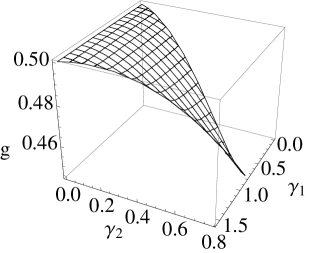
Figure 2: The minimum of $g(x_{3},\gamma_{1},\gamma_{2})$ over $x_{3}$ in each rank-two subspace; the global minimum is obtained at $\gamma_{1}=\gamma_{2}=\frac{\pi}{4}$.

Figure 1 shows $g(x_{3},\gamma_{1},\gamma_{2})$ as a function of $x_{3}$ for several different values of $\gamma_{1},\gamma_{2}$. $g(x_{3},\gamma_{1},\gamma_{2})$ is equal to $\frac{1}{2}\bigl{[}1+\cos(\gamma_{1}\mp\gamma_{2})\bigr{]}$ at $x_{3}=\pm 1$. This is consistent with the well-known result on GM of two-qubit pure states, which is a function of the concurrence; recall that the concurrence is equal to $\sin(\gamma_{1}\mp\gamma_{2})$ for the two states with $x_{3}=\pm 1$ em02 . $g(x_{3},\gamma_{1},\gamma_{2})$ is equal to $\frac{1}{2}$ at $x_{3}=0$, which is independent of the other two parameters. This observation implies that $G^{2}(|\psi\rangle)=\frac{1}{2}$ for any pure three-qubit state which is maximally entangled under some bipartite partition; a perfect example is the GHZ state. Once the value of $g(x_{3},\gamma_{1},\gamma_{2})$ is specified at the three points $x_{3}=\pm 1,0$, the value of $g(x_{3},\gamma_{1},\gamma_{2})$ at a generic point can roughly be estimated by interpolation, keeping the convexity of $g(x_{3},\gamma_{1},\gamma_{2})$ with respect to $x_{3}$ in mind. This simple picture is very useful in understanding the dependence of $g(x_{3},\gamma_{1},\gamma_{2})$ on various parameters, and why the W state is the maximally entangled state with respect to GM, as we shall see shortly.

It is interesting to note that, when $x_{3}>x_{3}^{(4)}$ or $x_{3}<x_{3}^{(3)}$, $g(x_{3},\gamma_{1},\gamma_{2})$ is a linear function of $x_{3}$, with positive and negative derivatives, respectively. Hence, for given $\gamma_{1},\gamma_{2}$, the minimum of $g(x_{3},\gamma_{1},\gamma_{2})$ is obtained in the interval $x_{3}^{(3)}\leq x_{3}\leq x_{3}^{(4)}$. When $\gamma_{2}=0$, $g(x_{3},\gamma_{1},\gamma_{2})$ is an even function of $x_{3}$; its minimum for given $\gamma_{1}$ is obtained at $x_{3}=0$ and is equal to $\frac{1}{2}$. Otherwise, the partial derivative of $g(x_{3},\gamma_{1},\gamma_{2})$ with respect to $x_{3}$ is positive at $x_{3}=0$; the minimum of $g(x_{3},\gamma_{1},\gamma_{2})$ for given $\gamma_{1},\gamma_{2}$ is obtained in the interval $x_{3}^{(3)}\leq x_{3}<0$ and is smaller than $\frac{1}{2}$. Setting the derivative of $g(x_{3},\gamma_{1},\gamma_{2})$ with respect to $x_{3}$ to zero leads to a fourth-order polynomial equation about $x_{3}$; the minimum can be found after solving this equation. In particular, $-1<x_{3}<0$ at the global minimum of $g(x_{3},\gamma_{1},\gamma_{2})$. Figure 2 shows the dependence of the minimum of $g(x_{3},\gamma_{1},\gamma_{2})$ over $x_{3}$ on $\gamma_{1},\gamma_{2}$; the minimum is also the minimum of $g(\rho_{\mathrm{rk}2})$ in the rank-two subspace. According to the figure, the global minimum of $g(x_{3},\gamma_{1},\gamma_{2})$ is obtained in the rank-two subspace with $\gamma_{1}=\gamma_{2}=\frac{\pi}{4}$.

To determine the maximally entangled multipartite states is a highly nontrivial task, since it usually involves a massive optimization process over a large parameter space. Even for three qubits, the maximally entangled state with respect to GM is not known for sure, although it has been conjectured with strong evidence that the W state is such a candidate twp09 . As an immediate application of the above results, we prove this conjecture rigorously in Appendix C.

Theorem 1

Up to local unitary transformations, the W state is the unique maximally entangled pure three-qubit state with respect to GM.

Theorem 1 can be generalized to mixed states according to the convex roof definition in Eq. (3).

Theorem 2

The W state is the maximally entangled state among all three-qubit states with respect to GM.

IV conclusions

We have provided analytical methods for deriving the GM of symmetric pure multiqubit states with non-negative amplitudes in the Dicke basis and that of symmetric pure three-qubit states. Also, we have introduced a systematic method for studying the GM of pure three-qubit states in virtue of a canonical form of their bipartite reduced states. In particular, we have derived explicit analytical formulae of GM for the family of pure three-qubit states one of whose rank-two two-qubit reduced states is a convex combination of the maximally entangled state and its orthogonal pure state within the rank-two subspace. Based on these results, we further proved that the W state is the maximally entangled three-qubit state with respect to GM. Our studies can simplify the calculation of GM and provide a better understanding of multipartite entanglement, especially the entanglement in three-qubit states. Our results also facilitate the comparison of GM with other entanglement measures, like relative entropy of entanglement hmm08 ; zch10 . Moreover, they may help investigate the physical phenomena in multipartite entangled systems emerging in condensed matter physics.

Appendix A: Derivation of Eqs. (II.2–II.2)

We will use the technique in Refs. tpt08 ; tkk09 to simplify the problem. According to the definition in Eq. (1),

$$G^{2}(|\Phi\rangle) =\underset{|a\rangle|b\rangle|c\rangle}{\mathrm{max}}\mathrm{Tr}\bigl{[}|\Phi\rangle\!\langle\Phi|\bigl{(}|a\rangle\!\langle a|\otimes|b\rangle\!\langle b|\otimes|c\rangle\!\langle c|\bigr{)}\bigr{]}$$

$$=\underset{|a\rangle|b\rangle}{\mathrm{max}}\;\mathrm{Tr}\bigl{[}\bigl{(}\text{Tr}_{C}|\Phi\rangle\!\langle\Phi|\bigr{)}\bigl{(}|a\rangle\!\langle a|\otimes|b\rangle\!\langle b|\bigr{)}\bigr{]},$$ (42)

where $|a\rangle,|b\rangle$ are normalized qubit states. The second equality follows from Theorem 1 of E. Jung et al. jung08 , which states that any ($n-1$)-qudit reduced state uniquely determines the GM of the original $n$-qudit pure state, as we have mentioned in the second paragraph of Sec. III.

To reduce Eq. (Appendix A: Derivation of Eqs. (–)), we use the Bloch sphere representation of qubit nc00 :

$$\rho:=\frac{1}{2}\left(I+\bm{s}_{\rho}\cdot\bm{\sigma}\right),$$ (43)

where the components of $\bm{\sigma}$ are three Pauli matrices and $\bm{s}_{\rho}$ is the Bloch vector.

Suppose the states $|a\rangle,|b\rangle$ have Bloch vectors $\bm{s}_{1},\bm{s}_{2}$ respectively. Then Eq. (Appendix A: Derivation of Eqs. (–)) gives rise to two sets of equations:

$$\bm{r}_{1}+G\bm{s}_{2}=\lambda_{1}\bm{s}_{1},\quad\bm{r}_{2}+G\bm{s}_{1}=\lambda_{2}\bm{s}_{2},$$

$$\bm{r}_{1}=\text{Tr}[\text{Tr}_{BC}(|\Phi\rangle\!\langle\Phi|)\bm{\sigma}],\quad\bm{r}_{2}=\text{Tr}[\text{Tr}_{AC}(|\Phi\rangle\!\langle\Phi|)\bm{\sigma}],$$ (44)

where $\lambda_{1},\lambda_{2}$ are Lagrange multipliers, and the $3\times 3$ matrix $G$ has elements $G_{ij}=\text{Tr}[(\text{Tr}_{C}|\Phi\rangle\!\langle\Phi|)(\sigma_{i}\otimes\sigma_{j})]$. Since the reduced density operators $\text{Tr}_{BC}|\Phi\rangle\!\langle\Phi|$ and $\text{Tr}_{AC}|\Phi\rangle\!\langle\Phi|$ are identical, one can show that $\bm{r}_{1}=\bm{r}_{2}=\bm{r}$ after some algebra. It follows that $\bm{s}_{1}=\bm{s}_{2}=\bm{s}$, $\lambda_{1}=\lambda_{2}=\lambda$, and Eq. (Appendix A: Derivation of Eqs. (–)) reduces to

$$\bm{r}+G\bm{s}=\lambda\bm{s}.$$ (45)

The solutions to Eq. (45) determine the GM of the state $|\Phi\rangle$ in Eq. (8).

Define $\bm{s}=(\sin\theta\cos\varphi,\sin\theta\sin\varphi,\cos\theta)$ with $\theta\in[0,\pi]$ and $\varphi\in[0,2\pi]$; then Eq. (45) reduces to Eqs. (II.2)–(II.2).

Appendix B: Derivation of Eq. (III.3)

In this Appendix, we derive Eq. (III.3). Recall that the relevant parameter range is $0\leq\gamma_{2}\leq\gamma_{1}\leq\frac{\pi}{2}$, $\gamma_{2}+\gamma_{1}\leq\frac{\pi}{2}$, and $-1\leq x_{3}\leq 1$, see Sec. III.1. To simplify the following discussion, we also assume $0<\gamma_{1}<\frac{\pi}{2}$ and $|x_{3}|<1$; but it turns out that the final result is applicable without this restriction.

When $x_{1}=x_{2}=0$, according to Eqs. (35) and (36),

$$f(a,b,c) = 1+c\cos\gamma_{1}\cos\gamma_{2}+cx_{3}\sin\gamma_{1}\sin\gamma_{2}+|\bm{w}|,$$

$$\bm{w} = \left(\begin{array}[]{c}a(\cos\gamma_{2}\sin\gamma_{1}-x_{3}\cos\gamma_{1}\sin\gamma_{2})\\ b(-x_{3}\cos\gamma_{2}\sin\gamma_{1}+\cos\gamma_{1}\sin\gamma_{2})\\ cx_{3}+x_{3}\cos\gamma_{1}\cos\gamma_{2}+\sin\gamma_{1}\sin\gamma_{2}\\ \end{array}\right)^{T}.$$ (49)

According to Sec. III.2, to compute $g(x_{3},\gamma_{1},\gamma_{2})$, or equivalently, the maximum of $f(a,b,c)$ over the unit sphere, we need only to maximize $f_{2}(c)=f(\sqrt{1-c^{2}},0,c)$ over the single variable $c$ for $-1\leq c\leq 1$. Here $f_{2}(c)$ can be expressed as follows,

$$f_{2}(c) = 1+u_{0}c+\sqrt{u_{1}c^{2}+2u_{2}c+u_{3}},$$

$$u_{0} = \cos\gamma_{1}\cos\gamma_{2}+x_{3}\sin\gamma_{1}\sin\gamma_{2}>0,$$

$$u_{1} = x_{3}^{2}-(\cos\gamma_{2}\sin\gamma_{1}-x_{3}\cos\gamma_{1}\sin\gamma_{2})^{2},$$

$$u_{2} = (x_{3}\cos\gamma_{1}\cos\gamma_{2}+\sin\gamma_{1}\sin\gamma_{2})x_{3},$$

$$u_{3} = (\sin\gamma_{1})^{2}+x_{3}^{2}(\cos\gamma_{1})^{2}>0.$$ (51)

The four coefficients $u_{0},u_{1},u_{2},u_{3}$ in Eq. (Appendix B: Derivation of Eq. ()) satisfy the following relations,

$$u_{2}>u_{1},\quad u_{2}^{2}-u_{1}u_{3}>0,\quad u_{0}^{2}-u_{1}>0;$$ (52)

these relations are useful in the following discussion.

To determine the maximum of $f_{2}(c)$ for $-1\leq c\leq 1$, we shall differentiate three cases according to the sign of $u_{1}$. Note that $u_{1}$ is a quadratic function of $x_{3}$ with a positive quadratic coefficient, and that it has the following two zeros:

$$x_{3}^{(1,2)}=\frac{\cos\gamma_{2}\sin\gamma_{1}}{\pm 1+\cos\gamma_{1}\sin\gamma_{2}},$$ (53)

which satisfy the inequalities: $-1\leq x_{3}^{(2)}<0<x_{3}^{(1)}<1$; $x_{3}^{(2)}$ is equal to $-1$ only if $\gamma_{1}+\gamma_{2}=1$.

Case 1: $x_{3}=x_{3}^{(1)}$ or $x_{3}=x_{3}^{(2)}$. In this case $u_{1}=0$, $u_{0},u_{2}>0$,

$$f_{2}(c) = 1+u_{0}c+\sqrt{2u_{2}c+u_{3}},$$ (54)

so the maximum of $f_{2}(c)$ can only be obtained at $c=1$.

Case 2: $x_{3}<x_{3}^{(2)}$ or $x_{3}>x_{3}^{(1)}$. In this case, $u_{0},u_{1},u_{2}>0$, the discriminant of the quadratic function $u_{1}c^{2}+2u_{2}c+u_{3}$ about $c$ is $4(u_{2}^{2}-u_{1}u_{3})>0$, so the quadratic function has two zeros with mean $-u_{2}/u_{1}<0$. Since the quadratic function must be nonnegative in the interval $[-1,1]$ by definition, both zeros must be smaller than or equal to $-1$. In the interval $[-1,1]$, this quadratic function and $f_{2}(c)$ are both strictly increasing, so the maximum of $f_{2}(c)$ can only be obtained at $c=1$.

Case 3: $x_{3}^{(2)}<x_{3}<x_{3}^{(1)}$. In this case $u_{1}<0$, the quadratic function $u_{1}c^{2}+2u_{2}c+u_{3}$ is positive between its two zeros. One zero is smaller than or equal to $-1$, and the other larger than or equal to 1. To determine the maximum of $f_{2}(c)$, we take the first and the second derivatives of $f_{2}(c)$:

$$f_{2}^{\prime}(c) = u_{0}+\frac{u_{1}c+u_{2}}{\sqrt{u_{1}c^{2}+2u_{2}c+u_{3}}},$$

$$f_{2}^{\prime\prime}(c) = \frac{u_{1}u_{3}-u_{2}^{2}}{(u_{1}c^{2}+2u_{2}c+u_{3})^{3/2}}<0,$$ (55)

where the last inequality follows from Eq. (52). There is only one solution to the equation $f_{2}^{\prime}(c)=0$,

$$\bar{c} = -\bigl{[}x_{3}^{2}-(\cos\gamma_{2}\sin\gamma_{1}-x_{3}\cos\gamma_{1}\sin\gamma_{2})^{2}\bigr{]}^{-1}$$ (56)

$$\times\bigl{[}x_{3}(x_{3}\cos\gamma_{1}\cos\gamma_{2}+\sin\gamma_{1}\sin\gamma_{2})$$

$$+\sin\gamma_{1}(\cos\gamma_{1}\cos\gamma_{2}+x_{3}\sin\gamma_{1}\sin\gamma_{2})$$

$$\times(\sin\gamma_{1}-x_{3}\cos\gamma_{1}\tan\gamma_{2})\bigr{]}\geq 0.$$

Since the second derivative of $f_{2}(c)$ is always negative, $\bar{c}$ is the global maximum of the function $f_{2}(c)$ in the interval where it is real valued. Restricted to the interval $[-1,1]$, the maximum of $f_{2}(c)$ is obtained at $\bar{c}$ if $\bar{c}<1$ and at $c=1$ otherwise. In both cases, the maximum point is unique. Hence, it remains to determine when $\bar{c}\geq 1$ and when $\bar{c}<1$.

After some algebra, one can show that $x_{3}^{(1,2)}$ defined in Eq. (53) and $x_{3}^{(3,4)}$ defined in Eq. (41) satisfy the following inequalities,

$$-1\leq x_{3}^{(2)}\leq x_{3}^{(3)}<0\leq x_{3}^{(4)}<x_{3}^{(1)}<1.$$ (57)

If $\gamma_{1}+\gamma_{2}=\frac{\pi}{2}$, then $x_{3}^{(3)}=x_{3}^{(2)}=-1$, and $\bar{c}$ satisfies the following relation,

$$\left\{\begin{array}[]{cl}\bar{c}<1&\quad-1<x_{3}<x_{3}^{(4)},\\ \bar{c}\geq 1&\quad x_{3}^{(4)}\leq x_{3}<x_{3}^{(1)}.\end{array}\right.$$ (60)

If $\gamma_{1}+\gamma_{2}<\frac{\pi}{2}$, then $-1<x_{3}^{(2)}<x_{3}^{(3)}$, and $\bar{c}$ satisfies the following relation,

$$\left\{\begin{array}[]{cl}\bar{c}<1&\quad x_{3}^{(3)}<x_{3}<x_{3}^{(4)},\\ \bar{c}\geq 1&\quad x_{3}^{(2)}<x_{3}\leq x_{3}^{(3)}\quad\mbox{or}\quad x_{3}^{(4)}\leq x_{3}<x_{3}^{(1)}.\end{array}\right.$$ (63)

According to the observations in the above three cases, if $-1<x_{3}\leq x_{3}^{(3)}$ or $x_{3}^{(4)}\leq x_{3}<1$, the maximum of $f_{2}(c)$ is obtained at 1; if $-x_{3}^{(3)}<x_{3}<x_{3}^{(4)}$, the maximum is obtained at $\bar{c}$. The maximum point is unique in both cases. The values of $f_{2}(c)$ at 1 and $\bar{c}$ are respectively given by

$$f_{2}\bigl{(}\bar{c}\bigr{)}=$$

$$\frac{2(1-x_{3}^{2})\sin\gamma_{1}\cos\gamma_{2}(\cos\gamma_{2}\sin\gamma_{1}-x_{3}\cos\gamma_{1}\sin\gamma_{2})}{-\bigl{[}x_{3}^{2}-(\cos\gamma_{2}\sin\gamma_{1}-x_{3}\cos\gamma_{1}\sin\gamma_{2})^{2}\bigr{]}},$$

$$f_{2}(1)=1+\cos\gamma_{1}\cos\gamma_{2}+x_{3}\sin\gamma_{1}\sin\gamma_{2}$$

$$\hphantom{f_{2}(1)=}+|x_{3}+x_{3}\cos\gamma_{1}\cos\gamma_{2}+\sin\gamma_{1}\sin\gamma_{2}|$$

$$\hphantom{f_{2}(1)}=\left\{\begin{array}[]{cc}(1-x_{3})[1+\cos(\gamma_{1}+\gamma_{2})],&\quad x_{3}\leq x_{3}^{(3)},\\ (1+x_{3})[1+\cos(\gamma_{1}-\gamma_{2})],&\quad x_{3}\geq x_{3}^{(4)},\end{array}\right.$$ (66)

where in deriving the last equality, we have noticed that

$$\left\{\begin{array}[]{cc}x_{3}+x_{3}\cos\gamma_{1}\cos\gamma_{2}+\sin\gamma_{1}\sin\gamma_{2}\leq 0,&\quad x_{3}\leq x_{3}^{(3)},\\ x_{3}+x_{3}\cos\gamma_{1}\cos\gamma_{2}+\sin\gamma_{1}\sin\gamma_{2}\geq 0,&\quad x_{3}\geq x_{3}^{(4)}.\end{array}\right.$$ (69)

Now Eq. (III.3) follows immediately when $0<\gamma_{1}<\frac{\pi}{2}$ and $|x_{3}|<1$; recall that $g(x_{3},\gamma_{1},\gamma_{2})=\frac{1}{4}\operatorname{max}_{-1\leq c\leq 1}f_{2}(c)$. It is straightforward to verify that the formula is also valid in the special cases $|x_{3}|=1$ or $\gamma_{1}=0,\frac{\pi}{2}$, hence the derivation is complete.

Appendix C: Proof of Theorem 1

To prove Theorem 1 in Sec. III.3, it suffices to show that the global minimum of $g(\rho_{\mathrm{rk}2})$ is obtained at the two-qubit reduced state of the W state.

In the relevant parameter range $0\leq\gamma_{2}\leq\gamma_{1}\leq\frac{\pi}{2}$, $\gamma_{1}+\gamma_{2}\leq\frac{\pi}{2}$, by taking its derivative with respect to $\gamma_{2}$ in Eq. (III.3), one can show that, for given $\gamma_{1},x_{3}$, $g(x_{3},\gamma_{1},\gamma_{2})$ is monotonically decreasing with $\gamma_{2}$ for $x_{3}<0$ and monotonically increasing with $\gamma_{2}$ for $x_{3}>0$. Assuming $x_{3}<0$, where the global minimum point should satisfy according to Sec. III.3; then $g(x_{3},\gamma_{1},\gamma_{2})$ is monotonically decreasing with $\gamma_{2}$. Hence, either $\gamma_{1}=\gamma_{2}$ or $\gamma_{1}+\gamma_{2}=\frac{\pi}{2}$ at the global minimum of $g(x_{3},\gamma_{1},\gamma_{2})$. We shall show that the unique minimum is obtained at the two-qubit reduced state of the W state in both cases.

IV.0.1 special case: $\gamma_{1}+\gamma_{2}=\frac{\pi}{2}$

If $\gamma_{2}=\frac{\pi}{2}-\gamma_{1}$ ($\frac{\pi}{4}\leq\gamma_{1}\leq\frac{\pi}{2}$), $\rho_{\mathrm{rk}2}$ is supported on the symmetrical subspace, according to Eqs. (III.1)–(III.1). In this case, Eq. (III.3) reduces to

$$g(x_{3},\gamma_{1},\frac{\pi}{2}-\gamma_{1})=$$

$$\left\{\begin{array}[]{cl}\frac{1}{2}-\frac{(1+x_{3})x_{3}(\cos\gamma_{1})^{2}}{-1+3x_{3}+(1+x_{3})\cos(2\gamma_{1})},&-1\leq x_{3}<x_{3}^{(4)},\vspace{0.5ex}\\ \frac{(1+x_{3})[1+\sin(2\gamma_{1})]}{4},&x_{3}^{(4)}\leq x_{3}\leq 1,\end{array}\right.$$ (72)

where

$$x_{3}^{(4)}=\frac{1-\sqrt{2}\sin(2\gamma_{1}+\frac{\pi}{4})}{3+\sqrt{2}\sin(2\gamma_{1}+\frac{\pi}{4})}.$$ (73)

$g(x_{3},\gamma_{1},\frac{\pi}{2}-\gamma_{1})$ is equal to $\frac{1}{2}$ at $x_{3}=0,-1$, independent of $\gamma_{1}$; $g(x_{3},\gamma_{1},\frac{\pi}{2}-\gamma_{1})$ is monotonically increasing with $\gamma_{1}$ for $-1<x_{3}<0$, and monotonically decreasing for $0<x_{3}\leq 1$ (see also Fig. 1).

To determine the maximum of $g(x_{3},\gamma_{1},\frac{\pi}{2}-\gamma_{1})$ for given $\gamma_{1}$, we can set its derivative with respect to $x_{3}$ to 0 (in the interval $-1\leq x_{3}<x_{3}^{(4)}$), which leads to the following quadratic equation over $x_{3}$,

$$[3+\cos(2\gamma_{1})]x_{3}^{2}+[-2+2\cos(2\gamma_{1})]x_{3}+\cos(2\gamma_{1})=1.$$

Given $\frac{\pi}{4}\leq\gamma_{1}\leq\frac{\pi}{2}$, the only solution with modulus less than or equal to 1 is

$$x_{3}^{(5)}=\frac{2\sin\gamma_{1}(\sin\gamma_{1}-\sqrt{2})}{3+\cos(2\gamma_{1})}.$$ (75)

The minimum of $g(x_{3},\gamma_{1},\frac{\pi}{2}-\gamma_{1})$ for given $\gamma_{1}$ is

$$g(x_{3}^{(5)},\gamma_{1},\frac{\pi}{2}-\gamma_{1})=\frac{[1+\cos(2\gamma_{1})+\sqrt{2}\sin\gamma_{1}]^{2}}{[3+\cos(2\gamma_{1})]^{2}}.$$ (76)

One can show that $g(x_{3}^{(5)},\gamma_{1},\frac{\pi}{2}-\gamma_{1})$ is monotonically increasing with respect to $\gamma_{1}$ by taking its derivative with respect to $\gamma_{1}$; hence, its minimum is obtained at $\gamma_{1}=\frac{\pi}{4}$. At this minimum point, $\gamma_{1}=\gamma_{2}=\frac{\pi}{4}$, $x_{3}=x_{3}^{(5)}=-\frac{1}{3}$, and $g(-\frac{1}{3},\frac{\pi}{4},\frac{\pi}{4})=\frac{4}{9}$. This minimum is also the global minimum of $g(\rho_{\mathrm{rk}2})$.

The rank-two state corresponding to this minimum is exactly the two-qubit reduced state of the W state, moreover, up to local unitary transformations, the W state is the only pure three-qubit state with this rank-two state as a two-qubit reduced state. To see this, recall that the two-qubit reduced state of $|\mathrm{W}\rangle=\frac{1}{\sqrt{3}}(|100\rangle+|010\rangle+|001\rangle)$ is

$$\rho_{\mathrm{rk}2}(\mathrm{W}) = \frac{1}{3}|00\rangle\langle 00|+\frac{2}{3}|\psi^{+}\rangle\langle\psi^{+}|$$ (77)

with $|\psi^{+}\rangle=\frac{1}{\sqrt{2}}(|01\rangle+|10\rangle)$, which is a convex combination of a pure product state and a orthogonal Bell state, thus $\gamma_{1}=\gamma_{2}=\frac{\pi}{4}$, according to Ref. em02 . In this rank-two subspace, the Bloch vectors of the two states $|00\rangle$ and $|\psi^{+}\rangle$ are $(0,0,1)$ and $(0,0,-1)$ respectively, and the Bloch vector of the state $\rho_{\mathrm{rk}2}(\mathrm{W})$ is exactly $(0,0,-\frac{1}{3})$.

IV.0.2 special case: $\gamma_{2}=\gamma_{1}\leq\frac{\pi}{4}$

In this case, Eq. (III.3) reduces to

$$g(x_{3},\gamma_{1},\gamma_{1})=$$

$$\left\{\begin{array}[]{cl}\frac{(1-x_{3})}{2}(\cos\gamma_{1})^{2},&-1\leq x_{3}\leq x_{3}^{(3)},\vspace{0.5ex}\\ \frac{-(1-x_{3})^{2}(1+x_{3})[\sin(2\gamma_{1})]^{2}}{-1+x_{3}(2+7x_{3})+(1-x_{3})^{2}\cos(4\gamma_{1})},&x_{3}^{(3)}<x_{3}<0,\vspace{0.5ex}\\ \frac{(1+x_{3})}{2},&0\leq x_{3}\leq 1,\end{array}\right.$$ (81)

where

$$x_{3}^{(3)}=-(\tan\gamma_{1})^{2}.$$ (83)

It is interesting to note that $g(x_{3},\gamma_{1},\gamma_{1})$ is independent of $\gamma_{1}$ when $0\leq x_{3}\leq 1$. If $x_{3}<0$, $g(x_{3},\gamma_{1},\gamma_{1})$ is monotonically decreasing with $\gamma_{1}$. Hence, $\gamma_{1}=\frac{\pi}{4}$ at its minimum, the corresponding rank-two subspace is then symmetric. According to the result on symmetric states in the previous subsection, the unique minimum of $g(x_{3},\gamma_{1},\gamma_{1})$ is also obtained at $\gamma_{1}=\gamma_{2}=\frac{\pi}{4}$, $x_{3}=-\frac{1}{3}$.

We have shown that the unique minimum of $g(x_{3},\gamma_{1},\gamma_{2})$ is obtained at $\gamma_{1}=\gamma_{2}=\frac{\pi}{4}$, $x_{3}=-\frac{1}{3}$, and that the corresponding state is the two-qubit reduced state of the W state. This minimum is also the global minimum of $g(\rho_{\mathrm{rk}2})$. To prove that the minimum is unique among all two-qubit rank-two states, it remains to show that it is unique in the rank-two subspace with $\gamma_{1}=\gamma_{2}=\frac{\pi}{4}$. It suffices to verify that $g(x_{1},x_{2},-\frac{1}{3},\frac{\pi}{4},\frac{\pi}{4})>g(0,0,-\frac{1}{3},\frac{\pi}{4},\frac{\pi}{4})$ for $x_{1}^{2}+x_{2}^{2}>0$ (here we write $g(x_{1},x_{2},x_{3},\gamma_{1},\gamma_{2})$ for $g(\rho_{\mathrm{rk}2})$). Due to the rotational symmetry of $g(x_{1},x_{2},x_{3},\gamma_{1},\gamma_{2})$ about the $x_{3}$ axis discussed in Sec. III.1, this is true if $g(x_{1},0,-\frac{1}{3},\frac{\pi}{4},\frac{\pi}{4})>g(0,0,-\frac{1}{3},\frac{\pi}{4},\frac{\pi}{4})$ for $x_{1}>0$. According to Eq. (36), when $\gamma_{1}=\gamma_{2}=\frac{\pi}{4}$, $x_{2}=0$, $x_{3}=-\frac{1}{3}$,

$$f\Bigl{(}\frac{2\sqrt{2}}{3},0,\frac{1}{3}\Bigr{)}=\frac{2}{9}\bigl{[}5+3x_{1}+\sqrt{9+3x_{1}(10+9x_{1})}\,\bigr{]};$$

hence,

$$g\Bigl{(}x_{1},0,-\frac{1}{3},\frac{\pi}{4},\frac{\pi}{4}\Bigr{)}\geq\frac{1}{4}f\Bigl{(}\frac{2\sqrt{2}}{3},0,\frac{1}{3}\Bigr{)},$$

$${}>\frac{4}{9}=g\Bigl{(}0,0,-\frac{1}{3},\frac{\pi}{4},\frac{\pi}{4}\Bigr{)}.$$ (85)

This completes the proof of Theorem 1.

References

- (1) A. Einstein, B. Podolsky, N. Rosen, Phys. Rev. 47, 777 (1935).
- (2) E. Schrödinger, Naturwissenschaften, 23, 807 (1935).
- (3) R. Horodecki, P. Horodecki, M. Horodecki, K. Horodecki, Rev. Mod. Phys. 81, 865 (2009).
- (4) R. Raussendorf and H. J. Briegel, Phys. Rev. Lett. 86, 5188 (2001); For a review on one-way quantum computation, see E. Campbell and J. Fitzsimons, arXiv:0906.2725 [quant-ph].
- (5) C. Y. Lu, W. B. Gao, O. Gühne, X. Q. Zhou, Z. B. Chen, and J. W. Pan, Phys. Rev. Lett. 102, 030502 (2009).
- (6) M. Hillery, V. Bužek, and A. Berthiaume, Phys. Rev. A 59, 1829 (1999).
- (7) V. Scarani, H. B. Pasquinucci, N. J. Cerf, M. Duâsek, N. Lütkenhaus, and M. Peev, Rev. Mod. Phys. 81, 001301 (2009).
- (8) C. H. Bennett, G. Brassard, C. Crépeau, R. Jozsa, A. Peres, and W. K. Wootters, Phys. Rev. Lett. 70, 1895 (1993).
- (9) D. M. Greenberger, M. A. Horne, and A. Zeilinger, in Bell’s Theorem, Quantum Theory, and Conceptions of the Universe, edited by M. Kafatos (Kluwer, Dordrecht, 1989), p. 69.
- (10) D. M. Greenberger, M. A. Horne, A. Shimony, and A. Zeilinger, Am. J. Phys. 58, 1131 (1990).
- (11) J. D. Bancal, C. Branciard, N. Gisin, and S. Pironio, Phys. Rev. Lett. 103, 090503 (2009).
- (12) R. Augusiak and P. Horodecki, Phys. Rev. A 80, 042307 (2009).
- (13) C. Y. Lu, X. Q. Zhou, O. Gühne, W. B. Gao, J. Zhang, Z. S. Yuan, A. Goebel, T. Yang, and J. W. Pan, Nat. Phys. 3, 91 (2007).
- (14) S. B. Papp, K. S. Choi, H. Deng, P. Lougovski, S. J. van Enk, H. J. Kimble, Science 324, 764 (2009).
- (15) R. H. Dicke, Phys. Rev. 93, 99 (1954).
- (16) W. Wieczorek, R. Krischek, N. Kiesel, P. Michelberger, G. Toth, and H. Weinfurter, Phys. Rev. Lett. 103, 020504 (2009).
- (17) R. Prevedel, G. Cronenberg, M. S. Tame, M. Paternostro, P. Walther, M. S. Kim, and A. Zeilinger, Phys. Rev. Lett. 103, 020503 (2009).
- (18) P. Krammer, H. Kampermann, D. Bruss, R. A. Bertlmann, L. C. Kwek, and C. Macchiavello, Phys. Rev. Lett. 103, 100502 (2009).
- (19) G. Vidal, J. Mod. Opt. 47, 355 (2000).
- (20) C. H. Bennett, D. P. DiVincenzo, J. A. Smolin, and W. K. Wootters, Phys. Rev. A 54, 3824 (1996).
- (21) For a review, see M. B. Plenio and S. Virmani, Quantum Inf. Comput. 7, 1 (2007).
- (22) M. A. Nielsen and I. L. Chuang, Quantum Computation and Quantum Information (Cambridge University Press, Cambridge, England, 2000).
- (23) T.-C. Wei and P. M. Goldbart, Phys. Rev. A 68, 042307 (2003).
- (24) D. C. Brody, and L. P. Hughston, J. Geom. Phys. 38, 19 (2001). The paper proposed the geometric measure of entanglement for bipartite pure states in an earilier version than wg03 .
- (25) D. A. Meyer and N. R. Wallach, J. Math. Phys. 43, 4273 (2002).
- (26) V. Coffman, J. Kundu and W. K. Wootters, Phys. Rev. A 61, 052306 (2000).
- (27) S. Tamaryan, T.-C. Wei and D. Park, Phys. Rev. A 80, 052315 (2009).
- (28) P. Facchi, G. Florio, G. Parisi, and S. Pascazio, Phys. Rev. A 77, 060304R (2008).
- (29) M. Hayashi, D. Markham, M. Murao, M. Owari, and S. Virmani, Phys. Rev. A 77, 012104 (2008).
- (30) M. Hayashi, D. Markham, M. Murao, M. Owari, and S. Virmani, Phys. Rev. Lett. 96, 040501 (2006).
- (31) D. Gross, S. T. Flammia, and J. Eisert, Phys. Rev. Lett. 102, 190501 (2009).
- (32) R. Orús, Phys. Rev. Lett. 100, 130502 (2008).
- (33) R. Orús, S. Dusuel, and J. Vidal, Phys. Rev. Lett. 101, 025701 (2008).
- (34) R. Orús, Phys. Rev. A 78, 062332 (2008).
- (35) R. Orús, and T.-C. Wei, arXiv:0910.2488 [cond-mat.str-el].
- (36) S. Tamaryan, H. Kim, M. S. Kim, K. S. Jang and D. K. Park, arXiv:0909.1077 [quant-ph].
- (37) L. Tamaryan, D. K. Park and S. Tamaryan, Phys. Rev. A 77, 022325 (2008).
- (38) J. J. Hilling and A. Sudbery, J. Math. Phys. 51, 072102 (2010).
- (39) P. Parashar, S. Rana, arXiv:0909.4443 [quant-ph].
- (40) X. Y. Chen, J. Phys. B: At. Mol. Opt. Phys. 43, 085507 (2010).
- (41) M. Hayashi, D. Markham, M. Murao, M. Owari, and S. Virmani, J. Math. Phys. 50, 122104 (2009).
- (42) R. Hübener, M. Kleinmann, T. -C. Wei, C. G. Guillén, and O. Gühne, Phys. Rev. A 80, 032324 (2009).
- (43) Y. Shimoni and O. Biham, Phys. Rev. A 75, 022308 (2007).
- (44) Y. Most, Y. Shimoni, O. Biham, Phys. Rev. A 81, 052306 (2010).
- (45) B.-G. Englert, N. Metwally, Kinematics of qubit pairs, in Mathematics of quantum computation, edited by R. K. Brylinski, G. Chen (Chapman & Hall/CRC Press, Boca Raton, 2002).
- (46) Huangjun Zhu, Lin Chen, and Masahito Hayashi, New J. Phys. 12, 083002 (2010).
- (47) Actually only two cases were handled in Ref. tkk09 . To compute the GM for the state with , it suffices to perform the phase gate on the state . So the states with and , respectively, have the same GM.
- (48) E. Jung, M.-R. Hwang, H. Kim, M.-S. Kim, D. K. Park, J.-W. Son, and S. Tamaryan, Phys. Rev. A 77, 062317 (2008).