Dynamics of Macroscopic Tunneling in Elongated BEC

Abstract

We investigate macroscopic tunneling from an elongated quasi 1-d trap, forming a ’cigar shaped’ BEC. Using recently developed formalismours1 we get the leading analytical approximation for the right hand side of the potential wall, i.e. outside the trap, and a formalism based on Wigner functions, for the left side of the potential wall, i.e. inside the BEC. We then present accomplished results of numerical calculations, which show a ’blip’ in the particle density traveling with an asymptotic shock velocity, as resulted from previous works on a dot-like trap, but with significant differences from the latter. Inside the BEC a pattern of a traveling dispersive shock wave is revealed. In the attractive case, we find trains of bright solitons frozen near the boundary.

I Introduction

In recent years, nonlinear dynamics of BEC out of equilibrium has been given a great amount of attention, mainly in looking for various nonlinear coherent structures such as dark, bright and oblique solitons, vortices and dispersive shock waves, and studying their emergence and evolution. Dark and bright solitons were first observed experimentally in Refs. darkso1, ; darkso2, ; brightso1, ; brightso2, . Vortices in 2d BECs were discussed in Refs. vortex1, ; vortex2, ; vortex3, ; vortex4, . Recently, much attention has been drawn to dispersive shock waves, which contrary to their dissipative counterparts in compressible fluid, and due to their quantum nature are controlled by the dispersion effects rather than by dissipation, and are now believed to emerge in and dictate the dynamics of BEC flow. They are characterized by an expanding oscillatory front, and, as other phenomena in BEC, are predicted and quested by the the Gross - Pitaevskii equation (GPE)

$$i\hbar\frac{\partial\Psi(r,t)}{\partial t}=$$

$$\left[-\frac{\hbar^{2}}{2m}\nabla^{2}+U_{ext}(r)+NU_{int}\mid\Psi(r,t)\mid^{2}\right]\Psi(r,t)$$ (1)

Recently dispersive shock waves in different BEC setups and with various initial conditions have been investigated and predicted theoretically, as well as observed in experiments. First evidence of possible shock waves development in BEC setups were reported in shock1 , where a sharp density depression was induced by slow light technique. Theoretical studies showed formation of a shock front in traveling 1-d BEC wave packets, split from an initial density perturbation in Refs. shock3a, and shock3b, . Shock waves in BEC induced by using Feshbach resonance were studied in Ref. shock4, and Witman averaging method was used to analyze 1-d BEC shock waves in the small dispersion limit in Ref. shock5, . Ref. shock2, presented imaging of rotating BEC ”blast waves” along with numerical analysis. A broad comparison between dispersive and dissipative shock waves in all dimensions was carried out in Ref. shock6, , which included examination of experimental reports and theoretical results. Study of supersonic flow past a macroscopic obstacle in 2-D BEC gave rise to predictions of a sonic Cherenkov cone that would eventually transform into spatial 2-d supersonic dispersive shock waves.shock7 Predictions of new 2-d creatures, called oblique solitons followed and are now an object of extensive studies in the field.shock8 ; shock9 . In Refs. fleischer1, ; fleischer2, , evidences of shock phenomena in macroscopic flow were found in nonlinear optics experiments.

In our previous worksours1 ; ours2 we studied tunneling from a trapped BEC Gaussian packet. For this purpose we analytically solved GPE in its hydrodynamic presentation. We showed that tunneling resulted in formation of an isolated ’blip’ in the particle density outside the trap, originating from a shock-type solution of the Burgers equation and moving with the asymptotic velocity of this shock. Experimental studies of the relevant phenomena in nonlinear optics were reported in Refs. bpss08, ; bpsss08, This effect is independent of the effect of non-linearity, i.e. inter-atomic interaction in BEC or Kerr nonlinearity optics, and includes the case in which the latter is zero.ours1 . This effect can be made repeatable in time by periodically bringing the potential walls closer (or changing the trap frequency) thus releasing additional blips with feasible control of their parameters, which may lead to an eventual realization of atom soliton laser.ours2 Since a strongly trapped BEC packet,(i.e. the margins of the trap are of the same order of magnitude as its bulk in all directions) reacts to tunneling in pulsations inside the trap, with frequency which is twice the in-trap eigen frequency, this periodicity is used to determine the timing of the mechanism described above. Sudden turn-on of a matter-wave source in order to create repeated pulses was discussed in Ref. CMM07, .

This paper will investigate tunneling from a quasi 1d cigar shaped trap with a twofold motivation: Firstly, we intend to look for the emergence of a single blip and its properties in order to eventually create a pulsed atom laser on the basis of this system, providing a much greater source of matter than in the previous case of tunneling from a trapped narrow packet (tightly trapped in all directions). Our second aim is to investigate the opposite effect, i.e. the dynamics inside the BEC cigar shaped trap, which appears to be much richer. We will show that an ”anti-blip” (a local depletion) is formed, which propagate inside the trap with the same velocity as the blip outside but in the opposite direction. However the structure and development of this anti-blip is very complicated and in particular it may develop into a dispersive shock wave.

II Model and Formalism

We consider the following physical system. An elongated 1d wave-function is sealed on its right hand side by a high enough wall, i.e. $U_{0}>NU_{int}\mid\psi(r,t)\mid^{2}$. (The quantum pressure term is always negative around the barrier region) The wall is lowered, at $t=0$, so that a tail of the wave function is allowed to tunnel and dynamically evolve according to the GPE through the new barrier of a finite width, the height of its peak is that of the former wall. This is shown in Fig. 1. We solve the 1-d GPE (I) numerically and analytically for the right and left sides of the barrier respectively, after $t=0$.

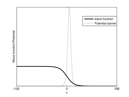
Figure 1: A schematic arrangement of the investigated problem. At $t=0$, the potential wall narrows down to a finite width barrier, enabling the cigar shaped BEC tail to tunnel

III Analytical results

III.1 Right hand side of the barrier

In our previous workours1 we introduced a formalism that solves GPE with a given external potential, in the hydrodynamic representation. The GPE is equivalently written in the form of the Euler type

$$v_{t}+\frac{1}{2}\nabla v^{2}=-\frac{1}{m}\left(-\frac{\hbar^{2}\nabla^{2}\sqrt{\rho}}{2m\sqrt{\rho}}+U_{ext}+NU_{int}\right)$$ (2)

and continuity

$$\rho_{t}+\nabla(\rho v)=0.$$ (3)

equations. Then the Euler equation (2) is solved under an adiabatic approximation according to which the density field $\rho=|\Psi|^{2}$ evolves with the time of tunneling $\tau_{tun}$ whereas the velocity field $m{\bf v}=\nabla\varphi$ ($\varphi$ being the gradient of the phase of wave function $\Psi$) with the traversal time $\tau_{tr}$ satisfying the condition $\tau_{tun}\gg\tau_{tr}$. The problem of a quantum fluid dynamics can be mapped onto that of a classical dissipationless fluid motion. We found out that solving the first iteration actually sufficed to investigate short and long time dynamics of the problem.

To investigate the dynamics outside the barrier in the present work, the analysis can be therefore made, as in the previous worksours1 by solving the classical integral

$$t=\int_{x_{0}}^{x}\frac{d\xi}{\sqrt{\frac{2}{m}(\epsilon-U(\xi))}}$$ (4)

where

$$U(\xi)=U_{t=0^{-}}(\xi)-U_{t=0^{+}}(\xi)=\frac{1}{2}U_{0}(1-\tanh(\alpha\xi)$$ (5)

is the difference between the potential shapes before and after switching from a wall to a barrier of finite width. $t$ is the time required for a fluid droplet (tracer) to reach the point $x$ and have velocity $v$, if it has started from the point $x_{0}$ with the energy $\epsilon$. Assuming that initially the fluid was motionless $v_{0}=0$ at $t=0$, i.e. $\epsilon=mv^{2}/2$, we get

$$\alpha t(x,\epsilon)=\frac{\mbox{arctanh}(\sqrt{\frac{\epsilon-\frac{1}{2}U_{0}+\frac{1}{2}U_{0}\tanh(\alpha x)}{\epsilon-U_{0}}})}{\sqrt{\epsilon-U_{0}}}+\frac{\mbox{arctanh}(\sqrt{\frac{\epsilon-\frac{1}{2}U_{0}+\frac{1}{2}U_{0}\tanh(\alpha x)}{\epsilon}})}{\sqrt{\epsilon}}$$ (6)

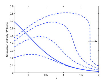
Figure 2: (Color online) Velocity field distribution at the first stages of tunneling from the cigar shaped trap. A tendency to shock formation is clearly observed. At $t=4$ there is a steep gradient (a jump) which indicates a transition to triple solution region

¿From here, one can find $\epsilon(x,t)$ numerically and therefore the velocity field $v(x,t)$. The results are shown in Fig. 2 and indicate, as expected, a tendency to shock wave formation (compare Refs. ours1, ; ours2, ) to result in a blip in the density distribution. The time scale of its creation is $4$ time units (traversal times $\tau_{tr}$) which matches that of the blip formation time to be obtained numerically.

III.2 Left hand side of the barrier

To deal with the dynamics to the left side of the barrier (inside the BEC) analytically, one can derive a hydrodynamic ”hole representation” by means of Wigner function technique. For this, let us assume that we have a homogeneous density distribution $\rho_{0}$ and consider fluctuations changing this density. In this case we have to define a ”hole Wigner function” as

$$f^{h}_{W}({\bf r},{\bf p},t)=$$

$$\int\frac{d^{3}y}{(2\pi\hbar)^{3}}\left[-\psi({\bf x}-{\bf y}/2,t)\psi^{*}({\bf x}+{\bf y}/2,t)+\rho_{0}\right]e^{i{\bf py}/\hbar}=$$

$$-f_{W}({\bf r},{\bf p},t)+\rho_{0}\delta({\bf p}).$$ (7)

We define the hole density by integrating (III.2) over the momentum p

$$\rho_{h}({\bf r},t)=\int d^{3}pf^{h}_{W}({\bf r},{\bf p},t)=-\rho({\bf r},t)+\rho_{0}$$ (8)

The hole velocity field is defined as

$$m_{0}\rho_{h}({\bf r},t)v^{\alpha}_{h}({\bf r},t)=\int d^{3}p\ p^{\alpha}f^{h}_{W}({\bf r},{\bf p},t)=$$

$$\rho_{h}({\bf r},t)\overline{p_{h}^{\alpha}}=-\rho({\bf r},t)\overline{p^{\alpha}}$$ (9)

Using definitions (III.2) and (8) we may write the density continuity equation in the form

$$\frac{\partial}{\partial t}\rho_{h}({\bf r},t)+\mbox{\boldmath$\nabla$}\cdot(\rho_{h}({\bf r},t){\bf v}_{h}({\bf r},t))=0.$$ (10)

In order to get the momentum continuity equation we first introduce the second conditional moments in the hole representation

$$\rho_{h}({\bf r},t)\overline{p_{h}^{\alpha}p_{h}^{\beta}}=\int d^{3}p\ p^{\alpha}p^{\beta}\ f^{h}_{W}({\bf r},{\bf p},t)=$$

$$\int d^{3}p\ p^{\alpha}p^{\beta}\ f_{W}({\bf r},{\bf p},t)=-\rho({\bf r},t)\overline{p^{\alpha}p^{\beta}}$$

and use the Liouville-Moyal equation

$$\frac{\partial}{\partial t}f_{W}({\bf r},{\bf p},t)=$$

$$\frac{1}{i\hbar}\{H({\bf r},{\bf p})\star f_{W}({\bf r},{\bf p},t)-f_{W}({\bf r},{\bf p},t)\star H({\bf r},{\bf p})\}$$ (11)

which governs the dynamics of Wigner function,m49 where

$$H({\bf r},{\bf p})=\frac{p^{2}}{2m}+V({\bf r})$$

is the classical Hamiltonian of the system. The definition of the $\star$ product and detailed discussion can be found in Ref. Z02, . Multiplying equation (III.2) by $p^{\alpha}$ and integrating over $p$ we get

$$-m_{0}\frac{\partial}{\partial t}[\rho_{h}({\bf r},t)v^{\alpha}_{h}({\bf r},t)]=$$

$$-\frac{\partial V({\bf x})}{\partial x^{\beta}}\rho({\bf r},t)\delta^{\alpha\beta}+\frac{1}{m_{0}}\frac{\partial}{\partial x^{\beta}}[\rho_{h}({\bf r},t)\overline{p_{h}^{\alpha}\ p_{h}^{\beta}}]$$ (12)

Then using the continuity equation (10) we write

$$-m_{0}\rho_{h}({\bf r},t)\frac{\partial v_{h}^{\alpha}({\bf r},t)}{\partial t}-m_{0}\rho_{h}({\bf r},t)\left[v_{h}^{\beta}({\bf r},t)\frac{\partial}{\partial x^{\beta}}\right]v_{h}^{\alpha}({\bf r},t)=$$

$$-\frac{\partial V({\bf x})}{\partial x^{\alpha}}\rho_{h}({\bf r},t)+\frac{1}{m_{0}}\frac{\partial}{\partial x^{\beta}}\left\{\rho_{h}({\bf r},t)\left[\overline{p_{h}^{\alpha}\ p_{h}^{\beta}}-\overline{p_{h}^{\alpha}}\ \overline{p_{h}^{\beta}}\right]\right\}$$ (13)

Till now no approximations have been made. But now we need an approximation that the holes can be described by the single wave function $\psi_{h}({\bf r},t)=f_{h}e^{-\frac{i}{\hbar}S_{h}}$ which can be justified for small values of the hole density $\rho_{h}({\bf r},t)<<\rho_{0}$. Then the standard procedure (see, e.g. Ref. lf01, ) results in

$$m_{0}\frac{\partial{\bf v}_{h}({\bf r},t)}{\partial t}+m_{0}\left[{\bf v}_{h}({\bf r},t)\cdot\mbox{\boldmath$\nabla$}\right]{\bf v}_{h}({\bf r},t)=$$

$$-\mbox{\boldmath$\nabla$}\left\{-\frac{\hbar^{2}}{2m_{0}}\frac{\mbox{\boldmath$\nabla$}^{2}f_{h}}{f_{h}}-V({\bf x})\right\}$$ (14)

which is the Euler equation for the holes similar to that for particles analyzed in Refs.ours1, ; ours2, . That is why in order to study the dynamics of tunneling inside the cigar shaped trap we may use the same technique as described in Ref. ours1, . Due to the symmetry of the problem we may directly apply equations (4) - (6) resulting in an emission of a blip in the empty space right of the barrier and come to the conclusions that simultaneously a depletion (an anti-blip) should be formed to the left of the barrier. It is expected to propagate to the left with the same velocity as the blip propagates to the right of the barrier.

However it is clear that the symmetry is not complete. In particular the density of particles to the right of the barrier cannot become negative. On the other hand, the density to the left may locally become higher than $\rho_{0}$, i.e. ”negative density of holes” is possible. Hence a more complicated behavior of the ”anti-blip” is expected. That is why below we carry out a detailed numerical study of the phenomenon.

IV Simulation

The simulation program solves dynamics of the system governed by GPE, and is based on Split Step Fourier and the Interaction Pictures Runge-Kutta-4 method.Ballagh . The initial conditions are chosen as follows. Since the macroscopic wave function is uniform throughout the elongated trap with a tunneling tail at the barrier, it was modeled as

$$\psi(x,0)=\frac{1-\tanh{\frac{x}{a}}}{b}$$ (15)

where $a$ and $b$ are parameters defining the slope of decay at the barrier, and the constant height inside the trap, respectively. The external potential barrier at the edge of the trap is taken as

$$U_{ext}(x)=\frac{U_{0}}{\cosh^{2}\frac{(x+\alpha)}{\beta}}$$ (16)

where $U_{0}$, $\alpha$ and $\beta$ are parameters that determine the height, shift from zero and width of the barrier, respectively. We consider weakly interacting BEC such that the interaction parameter $\frac{U_{int}|\psi|^{2}}{U_{0}}<1$ in the barrier region. This condition has to hold during the entire dynamical evolution, so that GPE remains valid.

IV.1 Right hand side of the barrier - Emergence of blip and splitting

As predicted by the analytical calculation, a blip emerges for all types of small interaction (repulsive, zero, and negative). Its initial velocity is strictly derived from the height of the barrier as $v=\sqrt{2U_{0}/m}$, also in the case of cigar shaped BEC as seen in Fig.3 However an interesting phenomenon arises, known to appear when super-Gaussian states are involved. Ref. gfvg08, shows using non-linear geometric optics method that an initial optical pulse of a super-Gaussian profile and high enough intensity, will eventually split in time into two shorter pulses. In accordance to the latter, splitting of the blip into two smaller blips under certain geometric parameters is obtained in the present work as well, where the split fractions propagate with velocities which roughly maintain momentum conservation of inelastic collision (if one ignores radiation): the mass of the original blip times its velocity equals the sum of masses times velocities of the split smaller blips. This is also seen in Fig. 3

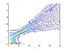
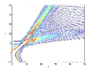
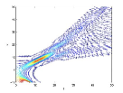
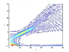
Figure 3: (Color online) 1-d space coordinate vs. time plot of numerical results showing emergence of the blip in the course of macroscopic tunneling from a cigar shaped trap. Upper figures relate to barrier height of $U_{0}=3$, whereas in lower figures $U_{0}=1$. Other trap parameters: $\alpha=3,\beta=4$. From right to left respectively: no, repulsive($U_{int}=3$) and attractive($U_{int}=-3$) interaction. Unlike in formerly investigates cases, i.e. tunneling from a narrow trap, a splitting of the blip into two components occurs right after its emergence.

IV.2 Inside the barrier - depletion

At the time the blip is created it leaves behind a depleted region, as was also shown in Refs. ours1, ; ours2, . This depletion enables consideration of the original problem as two separate problems in time and space, outside and inside the trap. The main difference between the previous and the present work is that while in the former this depletion was used to estimate the initial blip mass, in the latter it also indicates a compensating local rise of density in the trapped BEC near the barrier, which may ignite a shock propagation. If the symmetry had been complete there would have been no local increase of density inside the BEC but only an anti-blip that would have propagated as a dark soliton. Another interesting question is how long this depletion remains ’locked’ inside the barrier, and when does a tunneling tail starts to refilling it. The answer to this will be discussed below.

IV.3 Left hand side of the barrier - Anti-blip?

For repulsive interaction, an interesting case arises for which the tunneling process has almost perfect symmetry between the right and left sides of the barrier. This was discussed previously, in Sections III.2 and IV.2. In the former it was shown that if a local minimum of density inside the BEC is small enough, there is symmetry between the right and left side of the barrier. In this case one expects to see an anti-blip and an ’anti-ripple’ inside the BEC which propagate with the blip velocity, and which might even become a propagating dark soliton. This, of course, has to do with the proper geometry, and indeed seen in Fig.4 where an almost perfect symmetry between the propagating blip and anti-blip at $t=10$ is presented.

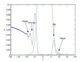
Figure 4: (Color online) An almost symmetrical blip - anti-blip solution appearing for the proper choice of trap parameters: $U_{0}=3,\alpha=1,\beta=2$ for small repulsive interaction($U_{int}=3$), at $t=10$.

IV.4 Left hand side of the barrier: dispersive shock wave?

An interesting observation is the dynamical evolution inside the BEC, which can be assigned to dispersive shock propagation in the systems controlled by GPE. It starts with depletion inside the barrier which remains locked until the BEC recovers, and a jump in the particle density inside the BEC to compensate for the depletion. This jump propagates accompanied, as is typical for dispersive shocks, by strong oscillations in its front, and leaving a slower rarefication behind. An important fact is that this is not sound propagation, as these shock waves evolve and propagate also in the limit of zero interaction when the sound velocity becomes zero. Let us examine the two other cases.

Repulsive interaction.

The dynamical solution inside the BEC for repulsive interaction is presented in Fig. 5. In this case a dispersive shock propagation is clearly observed. An important note is that the velocity of its front matches that of the blip, traveling on the right side of the barrier, and unlike in normal sound waves has no connection to the interaction strength. After long enough time the BEC exhibits a new equilibrium height, that might enable repeatable processes, Fig. 5.

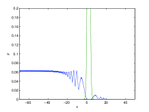
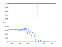
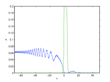
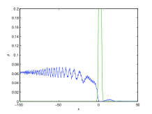
Figure 5: (Color online) Particle density vs. 1-d space coordinate plots show propagation of a jump in the particle density inside the BEC induced by tunneling for repulsive interaction. Increasing times from upper left figure are: $t=20,70,100,150$. This matches the dynamic behavior of dispersive shock propagation. In the course of the evolution it can be seen that the packet recovers to a new constant amplitude near the barrier, after it lost the blip mass.

Attractive interaction- localized train of bright solitons.

For attractive interaction a shock wave is eventually damped and does not propagate. Parts of the BEC become localized bright solitons shown in Fig. 6.

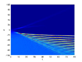
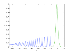
Figure 6: (Color online) Inside the BEC - attractive interaction case. A shock does not propagate, instead, localized bright solitons are formed. This is seen in both upper figure which shows 1-d space coordinate vs. time plot and lower figure which is a frozen density vs. 1-d space coordinate plot at $t=200$.

V Conclusions

In this work we have investigated the dynamics of macroscopic tunneling from an elongated cigar shaped trap. Several interesting phenomena were predicted by analytic formalisms and by numerics. As in the previous worksours1 ; ours2 on macroscopic tunneling, a blip in the particle density was shown to appear in the margins of the potential barrier and propagate with constant velocity, but contrary to other configurations, it was shown to split into two quite fast. Inside the BEC, dispersive shock waves that are now known to emerge in numerous configurations in BEC setups with repulsive interactions were predicted to appear, this time in macroscopic tunneling problems, and their velocity was shown to be easily controlled. In the case of attractive interaction bright solitons were shown to localize near the barrier. The BEC was also shown to stabilize near the barrier, which might enable realization of a soliton lasing from such a system. Symmetry and antisymmetry between the left and right hand sides of the barrier were discussed, and exhibited for a proper choice of parameters in a propagating ’anti- blip’ that might become a ’gray soliton’.

Acknowledgments. The authors acknowledge the support of United States - Israel Binational Science Foundation, Grant N 2006242. A.S. is partially supported by NSF. Hospitality of Max Planck Institute for Complex Systems, Dresden is highly appreciated.

References

- (1) G. Dekel, V. Fleurov, A. Soffer, C. Stucchio, Phys. Rev. A 75, 043617 (2007).
- (2) S. Burger, K. Bongs, S. Dettmer, W. Ertmer, K. Sengstock, A. Sanpera, G.V. Shlyapnikov and M. Lewenstein, Phys. Rev. Lett. 83, 5198 (1999).
- (3) J. Denschlag, J. E. Simsarian, D. L. Feder, Charles W. Clark, L. A. Collins, J. Cubizolles, L. Deng, E. W. Hagley, K. Helmerson, W. P. Reinhardt, S. L. Rolston, B. I. Schneider, and W. D. Phillips, Science 287, 97 (2000).
- (4) L. Khaykovich, F. Schreck, G. Ferrari, T. Bourdel, J. Cubizolles, L. D. Carr, Y. Castin, and C. Salomon, Science 296, 1290 (2002).
- (5) K. E. Strecker, G. B. Partridge, A. G. Truscott, R. G. Hulet, Nature(London) 417, 150 (2002).
- (6) M. R. Matthews, B. P. Anderson, P. C. Haljan, D. S. Hall, C. E. Wieman, and E. A. Cornell, Phys. Rev. Lett. 83, 2498 (1999).
- (7) B. P. Anderson, P. C. Haljan, C. E. Wieman, and E. A. Cornell, Phys. Rev. Lett. 85, 2857 (2000).
- (8) P. Engels, I. Coddington, P. C. Haljan, V. Schweikhard, and E. A. Cornell, Phys. Rev. Lett. 90, 170405 (2003).
- (9) R. Abo-Shaeer, C. Raman, J. M. Vogels, W. Ketterle, Science 292, 476 (2001).
- (10) Z. Dutton, M. Budde, C. Slowe, and L. V. Hau, Science 293, 663 (2001).
- (11) B. Damski, Phys. Rev. A. 69, 043610 (2004).
- (12) A.M. Kamchatnov, A. Gammal, R.A. Kraenkel, Phys. Rev. A. 69, 063605 (2004).
- (13) V. M. Perez-Garcia, V.V. Konotop, V.A. Brazhnyi, Phys Rev Lett 92, 220403 (2004).
- (14) F. K. Adbullaev, A. Gammal, A. M. Kamchatnov, L. Tomio, Int J Mod Phys B 19, 3415 (2005).
- (15) T. P. Simula, P. Engels, I. Coddington, V. Schweikhard, E. A. Cornell, R. J. Ballagh, Phys. Rev. Lett. 94, 080404 (2005). 350, 192 (2006).
- (16) M.A. Hoeffer, M.J. Ablowitz, I. Coddington, E.A. Cornell, P. Engels, V. Schweikhard, Phys. Rev. A 74, 023623 (2006).
- (17) G.A. El, A.M. Kamchatnov, Phys. Lett. A 352, 554-555 (2005).
- (18) G.A. El, A. Gammal, A.M. Kamchatnov, Phys. Rev. Lett. 97, 180405 (2006)
- (19) Yu. G. Gladush, G.A. El, A. Gammal, A.M. Kamchatnov, Phys. Rev. A 75, 033619 (2007).
- (20) W. Wan, S. Jia and J. W. Fleischer, Nature Physics 3, 46 (2007).
- (21) S. Jia, W. Wan, J.W. Fleischer, Phys. Rev. Lett. 99, 223901 (2007).
- (22) G. Dekel, O.V. Farberovich, A. Soffer, V. Fleurov, Physica D 238, 1475 (2009).
- (23) A. Barak, O. Peleg, A. Soffer, M. Segev, Opt.Lett. 33, 1798 (2008)
- (24) A. Barak, O. Peleg, C. Stucchio, A. Soffer, M. Segev Phys.Rev.Lett. 100, 153901 (2008)
- (25) A. del Campo, J. G. Muga, and M. Moshinsky, J. Phys. B: At. Mol. Opt. Phys. 40 975 (2007)
- (26) J. Moyal, Proc Cambridge Philos Soc 45, 99 (1949)
- (27) C. Zachos, Int. J. Mod. Phys. A17 297 (2002).
- (28) M. Levanda and V. Fleurov, Ann.Phys. NY 292, 199 (2001).
- (29) R.J. Ballagh, Computation methods for solving nonlinear partial differential equations. University of Otago (2000).
- (30) N. Gavish, G. Fibich, L.T. Vuong, and A.L. Gaeta, Phys. Rev. A 78, 043807 (2008).