Efficient Color-Dressed Calculation of Virtual Corrections

Abstract

With the advent of generalized unitarity and parametric integration techniques, the construction of a generic Next-to-Leading Order Monte Carlo becomes feasible. Such a generator will entail the treatment of QCD color in the amplitudes. We extend the concept of color dressing to one-loop amplitudes, resulting in the formulation of an explicit algorithmic solution for the calculation of arbitrary scattering processes at Next-to-Leading order. The resulting algorithm is of exponential complexity, that is the numerical evaluation time of the virtual corrections grows by a constant multiplicative factor as the number of external partons is increased. To study the properties of the method, we calculate the virtual corrections to $n$-gluon scattering.

Fermilab-PUB-09-406-T

1 Introduction

Automated Leading Order (LO) generators  [1, 2, 3, 4, 5] play an essential role in experimental analyses and phenomenology in general. However, the theoretical uncertainties associated with these generators are only understood qualitatively. The augmentation of the LO generators with Next-to-Leading Order (NLO) corrections will give a more quantitative understanding of the theoretical uncertainties. This is crucial for the realization of precision measurements at the Hadron colliders. By calculating NLO corrections using analytic generalized unitarity methods  [6, 7, 8], the one-loop amplitude is factorized into sums over products of on-shell tree-level amplitudes. This makes the integration of numerical generalized unitarity methods into the LO generators attractive. One can use the LO generator as the building block for obtaining the NLO correction, thereby negating the need for a separate generator of all the one-loop Feynman diagrams. The generalized unitarity approach reduces the complexity of the calculation through factorization. It can reduce the evaluation time with increasing number of external particles from faster than factorial growth to slower than factorial growth.

By utilizing the parametric integration method of Ref. [9] significant progress has been made in the algorithmic implementation of generalized unitarity based one-loop generators [10, 11] and other non-unitary methods [12]. These implementations rely on the color decomposition of the amplitude into colorless, gauge invariant ordered amplitudes [18, 19]. At tree-level these ordered amplitudes can be efficiently calculated by recursion relation algorithms [20]. These algorithms are of polynomial complexity and grow asymptotically as $n^{4}$ as the number of external partons, $n$, increases [21]. By replacing the 4-gluon vertex by an effective 3-gluon vertex the polynomial growth factor can be further reduced to $n^{3}$ [22, 23, 24].

At the one-loop level the ordered amplitudes generalize into primitive amplitudes [25]. These primitive amplitudes reflect the more complicated dipole structure of one-loop amplitudes. While the analytic structure of the factorized one-loop amplitude in color factors and primitive amplitudes is systematic, the subsequent calculation of the color summed virtual corrections becomes unwieldy in the algorithmic implementation [26]. The reason for this is the rapid growth in the number of primitive amplitudes. This rapid growth is mainly caused by the multiple quark-pairs amplitudes. A further complication arises from the possible presence of electro-weak particles in the ordered amplitudes.

While in LO generators the analytic treatment of color is more manageable, alternatives were developed for high parton multiplicity scattering amplitudes [23, 27, 24]. Those alternatives provided a more numerical treatment of the color, thereby facilitating the construction of tree-level Monte Carlo programs for the automated generation of high multiplicity parton scattering amplitudes at LO. This was accomplished by not only choosing the external momenta and helicities, but also choosing the explicit colors of the external partons for each scattering event considered. In doing so, the tree-level partonic amplitude is a complex number and the absolute value squared is simply calculated. This numerical treatment can be done in the context of ordered amplitudes [28] by calculating the explicit color weights of each ordered amplitude. This method was generalized to one-loop calculations in Ref. [12]. More directly, one can reformulate the recursion relations into color-dressed recursion relations [29, 23, 24]. These color-dressed recursion relations integrate the now explicit color weights into the recursive formula. The resulting algorithm is of exponential complexity and grows asymptotically as $4^{n}$ for $n$-parton amplitudes; again, a reduction of the growth factor to $3^{n}$ can be achieved if the 4-gluon vertex is replaced by the effective 3-gluon vertex [24].

In this paper we extend the generalized unitarity method of Ref. [10] as implemented in Ref. [30] to incorporate the color-dressing method. The algorithm is developed such that it can augment a dressed LO generator such as C OMIX  [5] to become a NLO generator. For the numerical examples presented in this paper, we have used our own implementation of a color-dressed LO gluon recursion relation to calculate the virtual corrections for $n$-gluon scattering processes.

The motivation for color dressing at the one-loop level is discussed in Sec. 2. We outline in Sec. 3 the tree-level dressed recursion relations for generic theories expressed in terms of Feynman diagrams. We optimize the color-sampling performance and study the phase-space integration convergence for LO $n$-gluon scattering. The dressed formalism is extended to one-loop amplitudes in Sec. 4. The scaling with $n$, the accuracy of the algorithm and the color-sampling convergence of the virtual corrections to $n$-gluon scattering are studied in some detail. We summarize our results in Sec. 5. Finally, two appendices are added giving an explicit LO 6-quark example and details on the color-dressed implementation of the gluon recursion relation.

2 Motivation for the Color-Dressed Generalized Unitarity Method

So far the numerical implementations of generalized unitarity for the evaluation of one-loop amplitudes make use of color ordering: the ordered one-loop amplitudes are constructed from tree-level ordered amplitudes through the $D$-dimensional unitarity cuts. This has the advantage that the color is factorized off the loop calculation and attached subsequently to each ordered one-loop amplitude. For the pure gluon one-loop amplitude, this leads to a particularly simple decomposition in terms of the adjoint generators $F$ of ${\rm SU}(N)$:

$${\cal M}^{(0,1)}(1,2\ldots,n)\ \ \sim\sum_{P(2,3,\ldots,n)}{\rm Tr}\left(F^{a_{1}}F^{a_{2}}\cdots F^{a_{n}}\right)m^{(0,1)}(1,2,\ldots,n)\ .$$ (1)

The decomposition is valid for both tree-level [18] and one-loop amplitudes [31]. Once we can calculate the colorless ordered amplitude $m(1,2,\ldots,n)$, all other ordered amplitudes are obtained by simple permutations. All kinematic information about the $n$-gluon amplitude is encapsulated in a single ordered amplitude. However, we also see the drawback of this approach as we are interested in evaluating the amplitude squared. We have to calculate ${\cal M}^{(0,1)}(1,2\ldots,n)\times\left({\cal M}^{(0)}(1,2\ldots,n)\right)^{\dagger}$ summed over all color and spin states of the external gluons. This immediately leads to a factorial complexity when doing the multiplications of the full amplitudes as we have to sum over the permutations, $P(2,3,\ldots,n)$, of the ordered amplitudes. Additionally, the color sum has to be performed either analytically or in some numerical manner.

When including quark pairs the situation becomes even more complicated. The reason is that the internal structure of the one-loop amplitude is not uniquely defined by the external states, thereby affecting the color flow of the ordered amplitudes. As a result there exist many types of ordered amplitudes depending on the internal configuration of quark and gluon propagators. These amplitudes are called primitive amplitudes [25] and in general cannot be obtained from each other by simple permutations. For example, the one-loop $q\bar{q}+n$ gluon amplitude is given by [31]

$${\cal M}^{(1)}(q;1,\ldots,n;\bar{q}\;\!)\ \ \sim$$ (2)

$$\sum_{k=2}^{n}\;\sum_{P(1,\ldots,n)}\left(T^{y}T^{a_{1}}\cdots T^{a_{k}}T^{x}\right)_{ij}\left(F^{a_{k+1}}\cdots F^{a_{n}}\right)_{xy}m^{(1)}(q,1,\ldots,k,q,k+1,\ldots,n)\ .$$

where the $T$-matrices are the fundamental generators of ${\rm SU}(N)$. While for the full amplitude a cut line has an undetermined flavor, each primitive amplitude has an unique flavor for all the cut lines. Therefore we can apply generalized unitarity to the primitive amplitudes. However, from a numerical/algorithmic point of view the evaluation of this equation becomes tedious as can be seen for instance in the calculation of the one-loop matrix elements for $W+5$ partons in Ref. [26].

It is clear that for an automated generator of one-loop corrections one would like to avoid ordered/primitive amplitudes altogether. For LO matrix elements, this can be done by applying the color-dressed recursion relations to evaluate the (unordered) tree-level amplitudes. From these color-dressed tree-level amplitudes we can build the one-loop color-dressed amplitudes by applying generalized unitarity, thereby circumventing the need for primitive amplitudes and explicit color summations. It is of interest to investigate the feasibility of this approach. The $n$-gluon scattering process is good for studying the behavior of the dressed algorithm. The color-ordered approach is most effective for $n$-gluon scattering. For processes with quark-pairs, the color-dressed approach will become even more efficient compared to the color-ordered approach.

An additional advantage of the color-dressed algorithm is that it treats partons and color neutral particles on the same footing. Specifically, we can include electro-weak particles without altering the algorithm. This is in contrast to the color-ordered algorithm, where the addition of electro-weak particles would lead to significant modifications in the algorithmic implementation of the method.

3 Dressed Recursive Techniques for Leading Order Amplitudes

In tree-level generators the Monte Carlo sampling over the external color and helicity states has become a standard practice  [23, 27, 24]. Such a color sampling allows for the efficient evaluation of large multiplicity partonic processes. A particular efficient implementation of the color-dressed Monte Carlo method uses the color-flow decomposition of the multi-parton amplitudes [23, 32, 24].

The principle of Monte Carlo sampling over the states of the external sources generalizes to any theory expressible through Feynman rules. By explicitly specifying the quantum numbers of the $n$ external sources, one can evaluate the tree-level amplitude squared and differential cross section using Monte Carlo sampling:

$$d\,\sigma_{\rm LO}(f_{1}f_{2}\rightarrow f_{3}\cdots f_{n})\ \ =$$ (3)

$$\frac{W_{\rm S}}{N_{\rm event}}\times\sum_{r=1}^{N_{\rm event}}d\,PS^{(r)}(K_{1}K_{2}\rightarrow K_{3}\cdots K_{n})\left|\;\!{\cal M}^{(0)}\left({\bf f}_{1}^{(r)},{\bf f}_{2}^{(r)},\ldots,{\bf f}_{n}^{(r)}\right)\right|^{2}\ ,$$

where

$${\bf f}_{i}^{(r)}\;=\;\left\{f_{i},h_{f_{i}},C_{f_{i}},K_{f_{i}}\right\}^{(r)}$$ (4)

denotes the flavor, spin, color and momentum four-vector of external state $i$ for event $r$. The constant $W_{\rm S}$ contains the appropriate identical particle factors and Monte Carlo sampling weights. For each event $r$, the external states are stochastically chosen such that when summed over many events we approximate the correct differential cross section with sufficient accuracy.

3.1 The Generic Recursive Formalism

To calculate the tree-level amplitude ${\cal M}^{(0)}$ in Eq. (3), we follow the method of color-dressed recursion relations as detailed in Refs. [24, 5]. A recursion relation builds multi-particle currents from other currents. The $m$-particle current $J_{\bf g}\left({\bf f}_{\pi}\right)$ has $m$ on-shell particles ${\bf f}_{\pi}=\{{\bf f}_{i}\}_{i\in\pi}=\{{\bf f}_{i_{1}},\ldots,{\bf f}_{i_{m}}\}$ where $\pi=\{i_{1},\ldots,i_{m}\}$ and one off-shell particle ${\bf g}=\left\{g,L_{g},C_{g},K_{g}\right\}$ with $g$, $L_{g}$, $C_{g}$ and $K_{g}$ denoting the flavor, Lorentz label, color and four-momentum, respectively. The momentum of the off-shell particle, $K_{g}$, is constrained by momentum conservation: $K_{g}=-K_{\pi}=-\sum_{i\in\pi}K_{i}$.

The dressed recursion relation generates currents using the propagators and interaction vertices of the theory. Using standard tensor notation we can write the propagators as

$$P^{{\bf g}_{1}{\bf g}_{2}}(Q) = \delta_{g_{1}g_{2}}\delta_{C_{g_{1}}C_{g_{2}}}P^{L_{g_{1}}L_{g_{2}}}(Q)\ ,$$

$$P^{{\bf g}}\big{[}J({\bf f}_{\pi})\big{]} = \sum_{{\bf g}_{1}}P^{{\bf g}{\bf g}_{1}}(K_{\pi})J_{{\bf g}_{1}}\big{(}{\bf f}_{\pi}\big{)}\ ,$$

$$P\big{[}J({\bf f}_{\pi_{1}}),J({\bf f}_{\pi_{2}})\big{]} = \sum_{{\bf g}_{1}{\bf g}_{2}}J_{{\bf g}_{1}}\big{(}{\bf f}_{\pi_{1}}\big{)}P^{{\bf g}_{1}{\bf g}_{2}}(K_{\pi_{1}})J_{{\bf g}_{2}}\big{(}{\bf f}_{\pi_{2}}\big{)}\ ,$$ (5)

where e.g. the gluon propagator is given by $P^{\mu_{1}\mu_{2}}(Q)=-g^{\mu_{1}\mu_{2}}/Q^{2}$. Note that the particle sums are taken over all quantum numbers of the off-shell particles ${\bf g}_{i}$. Furthermore, in all expressions momentum conservation is always implicitly understood. The on-shell tree-level $n$-particle amplitude can hence be expressed in terms of an $(n-1)$-current,

$${\cal M}^{(0)}\big{(}{\bf f}_{1},\ldots,{\bf f}_{n}\big{)}\;=\;P^{-1}\left[J\big{(}{\bf f}_{1},\ldots,{\bf f}_{n-1}\big{)},J\big{(}{\bf f}_{n}\big{)}\right]\ .$$ (6)

We denote the interaction vertices of the theory as $V_{{\bf g}_{1}\cdots{\bf g}_{k}}(Q_{1},\ldots,Q_{k})$. The maximal number of legs for the allowed vertices of the theory is denoted by $V_{\rm max}$. The number of legs of the vertex is indicated by the number of its arguments and the type of vertex is specified by the quantum numbers of the legs. The labels ${\bf g}_{1},\ldots,{\bf g}_{k}$ run over the values of all particles of the theory. Symmetries and renormalizability imply that many of the vertices are set to zero. The theory is defined by its particle content and its non-vanishing vertices, which are generalized tensors:

$$V_{{\bf g}_{1}\cdots{\bf g}_{k}}(Q_{1},\ldots,Q_{k})\;=\;V_{g_{1}\cdots g_{k};C_{g_{1}}\cdots C_{g_{k}}}^{L_{g_{1}}\cdots L_{g_{k}}}(Q_{1},\ldots,Q_{k})\ .$$ (7)

The sum of all vertices contracted in with currents constitutes the main building block of the recursion relation. We define it as

$$D_{\bf g}\big{[}J({\bf f}_{\pi_{1}}),\ldots,J({\bf f}_{\pi_{k}})\big{]}\;=\sum_{{\bf g}_{1}\cdots{\bf g}_{k}}V_{{\bf gg}_{1}\cdots{\bf g}_{k}}(K_{g}=-K_{\Pi_{k}},K_{\pi_{1}},\ldots,K_{\pi_{k}})\times J^{{\bf g}_{1}}\big{(}{\bf f}_{\pi_{1}}\big{)}\times\cdots\times J^{{\bf g}_{k}}\big{(}{\bf f}_{\pi_{k}}\big{)}\ ,$$ (8)

where the inclusive list $\Pi_{k}$ is build up of unions of the exclusive lists:

$$\Pi_{k}=\bigcup_{i=1}^{k}\pi_{i}\ .$$ (9)

Fig. 1 is a pictorial representation of Eq. (8) when using the example of QCD. For this case, we will work out the generic vertex blob in detail in the next subsection.

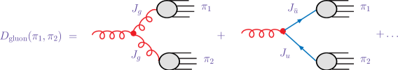
Figure 1: A graphical representation of Eq. (8) for $k=2$ and an off-shell gluon in QCD. Because of flavor conservation only one of the two vertices can contribute for any given partition.

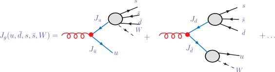
Figure 2: The first recursion step for the unordered gluon current with $u,\bar{d},s,\bar{s}$ quarks and a $W^{-}$ gauge boson in the final state. There are 15 contributions corresponding to all possible partitions of the final-state particles into two groups. Because of flavor conservation there are only 4 non-vanishing contributions for the “4+1” partitions (first term) and 2 non-vanishing contributions for the “3+2” partitions (second term).

The recursion relations terminate with the one-particle currents. A one-particle ${\bf g}$-current is defined in terms of the source $S^{h_{f_{i}}C_{f_{i}}}_{f_{i}L_{g}}(K_{f_{i}})$. Hence, we have

$$J_{\bf g}\big{(}{\bf f}_{i}\big{)}\;=\;\delta^{gf_{i}}\delta^{C_{g}C_{f_{i}}}\,S^{h_{f_{i}}C_{f_{i}}}_{f_{i}L_{g}}(K_{f_{i}})\ .$$ (10)

For example, the ${\bf g}_{1}$-gluon one-particle source with helicity $\lambda_{1}$, color $c_{1}$ and momentum $K_{1}$ is given by $J_{\bf g}({\bf g}_{1})=\delta^{cc_{1}}\epsilon^{\lambda_{1}}_{\mu_{1}}(K_{1})$. I.e. the ${\bf g}_{1}$-gluon source is a matrix in color space multiplied by the helicity vector.

The $n$-particle currents are now efficiently calculated from a recursively defined current in the following manner:

$$J_{\bf g}\big{(}{\bf f}_{1},\ldots,{\bf f}_{n}\big{)}\;=\;\sum_{k=2}^{V_{\rm max}-1}\sum_{P_{\pi_{1}\cdots\pi_{k}}(1,\ldots,n)}^{{\cal S}_{2}(n,k)}P_{\bf g}\Big{[}D\big{[}J({\bf f}_{\pi_{1}}),\ldots,J({\bf f}_{\pi_{k}})\big{]}\Big{]}\ ,$$ (11)

where ${\cal S}_{2}(n,k)$ is the Stirling number of the second kind. The first recursive step is graphically illustrated in Fig. (2) for the example of $J_{\bf g}({\bf u},{\bf\bar{d}},{\bf s},{\bf\bar{s}},{\bf W^{-}})$. The sum over $P_{\pi_{1}\cdots\pi_{k}}(1,\ldots,n)$ generates all different partitions decomposing the set $\{1,\ldots,n\}$ into the non-empty subsets $\pi_{1},\ldots,\pi_{k}$. An example for a list of different partitions is

$$P_{\pi_{1}\pi_{2}\pi_{3}}(1,2,3,4) = \left\{\pi_{1}^{(i)}\pi_{2}^{(i)}\pi_{3}^{(i)}\right\}_{i=1}^{{\cal S}_{2}(4,3)=6}$$ (12)

$$= \Big{\{}\ \big{\{}\{1,2\}\{3\}\{4\}\big{\}},\,\big{\{}\{1,3\}\{2\}\{4\}\big{\}},\,\big{\{}\{1,4\}\{2\}\{3\}\big{\}},$$

$$\hphantom{\Big{\{}\ }\big{\{}\{2,3\}\{1\}\{4\}\big{\}},\,\big{\{}\{2,4\}\{1\}\{3\}\big{\}},\,\big{\{}\{3,4\}\{1\}\{2\}\big{\}}\ \Big{\}}\ .$$

The formalism described here fully specifies an automated algorithm of exponential complexity to calculate the LO differential cross-sections for any theory defined in terms of Feynman rules. Owing to the characteristics of the partitioning, the computer resources needed to calculate the $n$-particle tree-level amplitudes asymptotically grow in proportion to ${\cal S}_{2}(n,V_{\rm max})$. The exponential behavior arises from the large-$n$ limit of the Stirling numbers, i.e. ${\cal S}_{2}(n,V_{\rm max})\rightarrow V_{\rm max}^{n}$ [22]. It may be possible to reduce $V_{\rm max}$ by rewriting higher multiplicity vertices as sums of lower multiplicity vertices thereby improving the efficiency of the recursive algorithm [23, 24]. For the case of the Standard model this has been fully worked out in Ref. [5] and implemented in the C OMIX LO generator.

3.2 Multi-Jet Scattering Amplitudes

We specify the generic recursion relations to the perturbative QCD Feynman rules. This will give an algorithmic description of the scattering amplitudes at LO for multi-jet production at hadron colliders.

The external sources are gluons and massless quarks. All these particles have color and helicity as quantum numbers. Instead of the traditional color representation in terms of fundamental generators, we choose the color-flow representation [3, 32, 24], which is more pertinent to Monte Carlo sampling and easily derivable from the traditional color representation by making the following two observation: first, any internal propagating gluon has as a color factor $\delta^{ab}={\rm Tr}\Big{(}T^{a}T^{b}\Big{)}$. This color factor can be rewritten as

$${\cal M}\;=\;{\cal A}_{a}\frac{\delta^{ab}}{K^{2}}{\cal B}_{b}\;=\;{\cal A}_{a}\frac{{\rm Tr}\left(T^{a}T^{b}\right)}{K^{2}}{\cal B}_{b}\;=\;{\cal A}_{ij}\frac{1}{K^{2}}{\cal B}^{ji}\ .$$ (13)

Second, we contract the amplitude with $T^{a_{k}}_{i_{k}j_{k}}$ for each external gluon:

$$|{\cal M}|^{2}\;=\;{\cal M}^{a}\,\delta_{ab}\left({\cal M}^{b}\right)^{\dagger}\;=\;{\cal M}^{a}\,T^{a}_{ij}T^{b}_{ji}\left({\cal M}^{b}\right)^{\dagger}\;=\;{\cal M}_{ij}\,{\cal M}_{ji}^{\dagger}\ .$$ (14)

From these observations it follows that we can calculate the interaction vertices in the color-flow representation by simply contracting each gluon with $T^{a_{k}}_{i_{k}j_{k}}$ and summing over $a_{k}$. The three gluon vertex is thus given by

$$V_{{\bf g}_{1}{\bf g}_{2}{\bf g}_{3}}(K_{1},K_{2},K_{3}) = V_{i_{1}j_{1}i_{2}j_{2}i_{3}j_{3}}^{\mu_{1}\mu_{2}\mu_{3}}(K_{1},K_{2},K_{3})$$ (15)

$$= T^{a_{1}}_{i_{1}j_{1}}T^{a_{2}}_{i_{2}j_{2}}T^{a_{3}}_{i_{3}j_{3}}\,V_{a_{1}a_{2}a_{3}}^{\mu_{1}\mu_{2}\mu_{3}}(K_{1},K_{2},K_{3})$$

$$= T^{a_{1}}_{i_{1}j_{1}}T^{a_{2}}_{i_{2}j_{2}}T^{a_{3}}_{i_{3}j_{3}}\,f^{a_{1}a_{2}a_{3}}\,\sqrt{2}\,\widehat{V}_{3}^{\mu_{1}\mu_{2}\mu_{3}}(K_{1},K_{2},K_{3})$$

$$= \left(\delta^{i_{1}}_{j_{2}}\delta^{i_{2}}_{j_{3}}\delta^{i_{3}}_{j_{1}}-\delta^{i_{1}}_{j_{3}}\delta^{i_{2}}_{j_{1}}\delta^{i_{3}}_{j_{2}}\right)\widehat{V}_{3}^{\mu_{1}\mu_{2}\mu_{3}}(K_{1},K_{2},K_{3})\ ,$$

with

$$\widehat{V}_{3}^{\mu_{1}\mu_{2}\mu_{3}}(K_{1},K_{2},K_{3})\;=\;\frac{1}{\sqrt{2}}\Big{(}(K_{1}-K_{2})^{\mu_{3}}g^{\mu_{1}\mu_{2}}+(K_{2}-K_{3})^{\mu_{1}}g^{\mu_{2}\mu_{3}}+(K_{3}-K_{1})^{\mu_{2}}g^{\mu_{3}\mu_{1}}\Big{)}\ .$$ (16)

Similarly, for the four gluon vertex we find

$$V_{{\bf g}_{1}{\bf g}_{2}{\bf g}_{3}{\bf g}_{4}}\;=\;V_{i_{1}j_{1}i_{2}j_{2}i_{3}j_{3}i_{4}j_{4}}^{\mu_{1}\mu_{2}\mu_{3}\mu_{4}}\;=\sum_{C(234)}\left(\delta^{i_{1}}_{j_{2}}\delta^{i_{2}}_{j_{3}}\delta^{i_{3}}_{j_{4}}\delta^{i_{4}}_{j_{1}}+\delta^{i_{1}}_{j_{4}}\delta^{i_{2}}_{j_{1}}\delta^{i_{3}}_{j_{2}}\delta^{i_{4}}_{j_{3}}\right)\widehat{V}_{4}^{\mu_{1}\mu_{3},\,\mu_{2}\mu_{4}}\ ,$$ (17)

with

$$\widehat{V}_{4}^{\mu_{1}\mu_{2},\,\mu_{3}\mu_{4}}\;=\;2\,g^{\mu_{1}\mu_{2}}g^{\mu_{3}\mu_{4}}-g^{\mu_{1}\mu_{3}}g^{\mu_{2}\mu_{4}}-g^{\mu_{1}\mu_{4}}g^{\mu_{2}\mu_{3}}\ ,$$ (18)

and the sum is over the cyclic permutation of the indices $\{2,3,4\}$. In the color-flow representation the quark-antiquark-gluon vertex is given by

$$V_{\bf qg\bar{q}}\;=\;V_{i,\,i_{1}j_{1},\,j}^{s\mu\bar{s}}\;=\;\left(\delta_{ij_{1}}\delta_{i_{1}j}-\frac{1}{N_{\rm C}}\,\delta_{i_{1}j_{1}}\delta_{ij}\right)\widehat{V}^{s\mu\bar{s}}\ ,$$ (19)

with

$$\widehat{V}_{s\bar{s}}^{\mu}\;=\;\frac{1}{\sqrt{2}}\,\gamma_{s\bar{s}}^{\mu}\ .$$ (20)

The external sources are given by

$$J_{\bf g}({\bf g}_{1}) = \delta^{Ii_{1}}\delta^{Jj_{1}}\varepsilon_{\mu}^{\lambda_{1}}(K_{1})\ ,$$

$$J_{\bf q}({\bf q}_{1}) = \delta^{Ii_{1}}v_{s}^{\lambda_{1}}(K_{1})\ ,$$

$$J_{\bf\bar{q}}({\bf\bar{q}}_{1}) = \delta^{Jj_{1}}\bar{u}_{\bar{s}}^{\lambda_{1}}(K_{1})\ ,$$ (21)

where ${\bf g}=\{g,\mu,(IJ),-K_{1}\}$, ${\bf g}_{1}=\{g_{1},\lambda_{1},(i_{1}j_{1}),K_{1}\}$, ${\bf q}=\{q,s,I,-K_{1}\}$, ${\bf q}_{1}=\{q_{1},\lambda_{1},i_{1},K_{1}\}$, ${\bf\bar{q}}=\{\bar{q},\bar{s},J,-K_{1}\}$ and ${\bf\bar{q}}_{1}=\{\bar{q}_{1},\lambda_{1},j_{1},K_{1}\}$. The internal propagating particles are given by

$$P^{{\bf g}_{1}{\bf g}_{2}}(Q) = \delta^{i_{1}}_{j_{2}}\delta^{i_{2}}_{j_{1}}\left(\frac{-g_{\mu_{1}\mu_{2}}}{Q^{2}}\right)\ ,$$

$$P^{{\bf q}_{1}{\bf q}_{2}}(Q) = \delta^{i_{1}}_{i_{2}}\left(Q\!\!\!\!/\,-m_{q_{1}}\right)^{-1}_{s_{1}s_{2}}\ ,$$

$$P^{{\bf\bar{q}}_{1}\bar{\bf q}_{2}}(Q) = \delta^{j_{1}}_{j_{2}}\left(Q\!\!\!\!/\,+m_{\bar{q}_{1}}\right)^{-1}_{\bar{s}_{1}\bar{s}_{2}}\ .$$ (22)

with ${\bf g}_{k}=\{g_{k},\mu_{k},(i_{k}j_{k}),Q\}$, ${\bf q}_{k}=\{q_{k},s_{k},i_{k},Q\}$ and ${\bf\bar{q}}_{k}=\{\bar{q}_{k},\bar{s}_{k},j_{k},Q\}$.

We can now construct Berends–Giele recursion relations [20] using color-dressed multi-parton currents based on Eq. (11). The result is

$$J_{\bf q}\big{(}{\bf f}_{1},\ldots,{\bf f}_{n}\big{)} = \sum_{P_{\pi_{1}\pi_{2}}(1,\ldots,n)}P_{\bf q}\Big{[}D\big{[}J({\bf f}_{\pi_{1}}),J({\bf f}_{\pi_{2}})\big{]}\Big{]}\ ,$$

$$J_{\bf g}\big{(}{\bf f}_{1},\ldots,{\bf f}_{n}\big{)} = \sum_{P_{\pi_{1}\pi_{2}}(1,\ldots,n)}P_{\bf g}\Big{[}D\big{[}J({\bf f}_{\pi_{1}}),J({\bf f}_{\pi_{2}})\big{]}\Big{]}\ ,$$ (23)

$$+ \sum_{P_{\pi_{1}\pi_{2}\pi_{3}}(1,\ldots,n)}P_{\bf g}\Big{[}D\big{[}J({\bf f}_{\pi_{1}}),J({\bf f}_{\pi_{2}}),J({\bf f}_{\pi_{3}})\big{]}\Big{]}\ ,$$

where each current violating flavor conservation is defined to give zero. The compact operator language can be expanded out to an explicit formula by adding back in the particle attributes. For example,

$$P_{\bf g}\Big{[}D\big{[}J({\bf f}_{\pi_{1}}),J({\bf f}_{\pi_{2}})\big{]}\Big{]} = \sum_{{\bf qg}_{1}{\bf\bar{q}}}P_{{\bf gg}_{1}}(K_{\Pi_{2}})\,V^{{\bf qg}_{1}{\bf\bar{q}}}\,J_{\bf q}({\bf f}_{\pi_{1}})\,J_{\bf\bar{q}}({\bf f}_{\pi_{2}})$$ (24)

$$+ \sum_{{\bf g}_{1}{\bf g}_{2}{\bf g}_{3}}P_{{\bf gg}_{1}}(K_{\Pi_{2}})\,V^{{\bf g}_{1}{\bf g}_{2}{\bf g}_{3}}(-K_{\pi_{1}\cup\pi_{2}},K_{\pi_{1}},K_{\pi_{2}})\,J_{{\bf g}_{2}}({\bf f}_{\pi_{1}})\,J_{{\bf g}_{3}}({\bf f}_{\pi_{2}})$$

$$= \frac{1}{K_{\Pi_{2}}^{2}}V^{s_{1}\mu s_{2}}_{i,\,IJ,\,j}\times J_{s_{1}}^{i}({\bf f}_{\pi_{1}})\times J_{s_{2}}^{j}({\bf f}_{\pi_{2}})$$

$$+ \frac{1}{K_{\Pi_{2}}^{2}}V^{\mu\mu_{1}\mu_{2}}_{IJi_{2}j_{2}i_{3}j_{3}}(-K_{\pi_{1}\cup\pi_{2}},K_{\pi_{1}},K_{\pi_{2}})\times J_{\mu_{1}}^{(ij)_{2}}({\bf f}_{\pi_{1}})\times J_{\mu_{2}}^{(ij)_{3}}({\bf f}_{\pi_{2}})\ .$$

The $n$-parton tree-level matrix element is calculated using Eq. (6). We exemplify in appendix A how to work out the 6-quark recursion steps using the above formalism.

3.3 Numerical Implementation of $n$-gluon Scattering

The method of color dressing as discussed in this section relies on the ability to perform a Monte Carlo sampling over the degrees of freedom of the external sources. In this subsection we will study in some detail the properties of such a sampling approach by means of the color-dressed gluonic recursion relation. We are particularly interested in the accuracy of the color-sampling procedure and overall speed of the implementation. The addition of quarks and external vector bosons is a straightforward extension and will not affect the conclusions reached in this subsection.

The explicit color-dressed gluon recursion algorithm is given in terms of colored gluonic currents. The gluonic currents are $3\times 3$ matrices in color space and defined as

$$J_{\bf g}\big{(}{\bf g}_{m}\big{)} = \delta^{Ii_{m}}\delta^{Jj_{m}}\,\varepsilon_{\mu}^{\lambda_{m}}(K_{m})\ ,$$

$$J_{\bf g}\big{(}{\bf g}_{1},\ldots,{\bf g}_{m}\big{)} = \sum_{P_{\pi_{1}\pi_{2}}(1,\ldots,m)}P_{\bf g}\Big{[}D\big{[}J({\bf g}_{\pi_{1}}),J({\bf g}_{\pi_{2}})\big{]}\Big{]}$$ (25)

$$+ \sum_{P_{\pi_{1}\pi_{2}\pi_{3}}(1,\ldots,m)}P_{\bf g}\Big{[}D\big{[}J({\bf g}_{\pi_{1}}),J({\bf g}_{\pi_{2}}),J({\bf g}_{\pi_{3}})\big{]}\Big{]}\ .$$

The color-dressed $n$-gluon amplitude is given by

$${\cal M}^{(0)}\big{(}{\bf g}_{1},{\bf g}_{2},\ldots,{\bf g}_{n}\big{)}\;=\;P^{-1}\left[J\big{(}{\bf g}_{1},{\bf g}_{2},\ldots,{\bf g}_{n-1}\big{)},J\big{(}{\bf g}_{n}\big{)}\right]\ .$$ (26)

For this specific example, we have labelled the on-shell gluons by ${\bf g}_{i}$, the off-shell gluon is denoted by ${\bf g}$ as before. The operator formulation of the recursive algorithm is particularly suited for an object oriented implementation of the recursive algorithm. We have implemented the algorithm presented above in C++. More details including the more explicit recursion equation are shown in appendix B.

The first issue to deal with is the correctness of the implemented algorithm. To this end we want to compare the color-dressed amplitude to existing evaluations of the gluonic amplitudes based on ordered amplitudes. To facilitate the comparison, we write the color-ordered expansion of the amplitude using the color-flow representation [32]:

$${\cal M}^{(0)}\big{(}{\bf g}_{1},{\bf g}_{2},\ldots,{\bf g}_{n}\big{)} = \sum_{P(2,\ldots,n)}{A^{(0)}}^{i_{1}\cdots i_{n}}_{j_{1}\cdots j_{n}}(g_{1}^{\lambda_{1}},\ldots,g_{n}^{\lambda_{n}})$$ (27)

$$= T^{a_{1}}_{i_{1}j_{1}}\cdots T^{a_{n}}_{i_{n}j_{n}}\sum_{P(2,\ldots,n)}\mbox{Tr}\big{(}F^{a_{1}}\cdots F^{a_{n}}\big{)}\;m^{(0)}(g_{1}^{\lambda_{1}},\ldots,g_{n}^{\lambda_{n}})$$

$$= \frac{1}{2}\sum_{P(2,\ldots,n)}\Big{(}\delta^{i_{1}}_{j_{2}}\delta^{i_{2}}_{j_{3}}\cdots\delta^{i_{n-1}}_{j_{n}}\delta^{i_{n}}_{j_{1}}+(-1)^{n}\,\delta^{i_{n}}_{j_{n-1}}\delta^{i_{n-1}}_{j_{n-2}}\cdots\delta^{i_{2}}_{j_{1}}\delta^{i_{1}}_{j_{n}}\Big{)}\;m^{(0)}(g_{1}^{\lambda_{1}},\ldots,g_{n}^{\lambda_{n}})$$

$$= \sum_{P(2,\ldots,n)}\delta^{i_{1}}_{j_{2}}\delta^{i_{2}}_{j_{3}}\cdots\delta^{i_{n-1}}_{j_{n}}\delta^{i_{n}}_{j_{1}}\;m^{(0)}(g_{1}^{\lambda_{1}},\ldots,g_{n}^{\lambda_{n}})\ .$$

The $m^{(0)}(g_{1}^{\lambda_{1}},\ldots,g_{n}^{\lambda_{n}})$ are ordered amplitudes with the property $m^{(0)}(1,2,\ldots,n)=(-1)^{n}\,m^{(0)}(n,\ldots,2,1)$. From the above formulas it follows that ${A^{(0)}}^{i_{1}\cdots i_{n}}_{j_{1}\cdots j_{n}}={A^{(0)}}^{j_{1}\cdots j_{n}}_{i_{1}\cdots i_{n}}$. By choosing the explicit momentum, helicity and color $(ij)_{m}$ of each gluon we can compare the numerical values of Eqs. (26) and (27). We have done the comparison up to $2\rightarrow 12$ gluon amplitudes and found complete agreement, thereby validating the correctness of the color-dressed algorithm.

An important consideration in calculating the color-dressed amplitudes is the color-sampling method used in the Monte Carlo program. For a $2\rightarrow n-2$ gluon scattering amplitude, each of the gluon color states is stochastically chosen. The full color configuration of the event is expressed by $\{(ij)_{m}\}_{m=1}^{n}$ where $i_{m}$ and $j_{m}$ each denote a color state out of three possible ones that can be labelled $\{1,2,3\}$. In the “Naive” approach one samples uniformly over all possible color states of the gluons. The number of color configurations, $N^{\rm Naive}_{\rm col}$, and the color-configuration weight, $W^{\rm Naive}_{\rm col}$, are given by

$$N^{\rm Naive}_{\rm col}\;=\;9^{n}$$ (28)

and

$$W^{\rm Naive}_{\rm col}\;=\;1\ ,$$ (29)

respectively. About 95% of the naive color configurations have a vanishing color factor. This results in a rather inefficient Monte Carlo procedure when sampling over the color states. As was noted in Ref. [24], a significant number of the zero color-weight configurations can be removed by imposing color conservation. This is implemented by vetoing any color configuration for which the condition $\exists\,c\in\{1,2,3\}:\sum_{m=1}^{n}\left(\delta_{i_{m},c}-\delta_{j_{m},c}\right)\neq 0$ is true. In other words, the non-vetoed color configurations can be obtained by uniformly choosing the colors $i_{1},\ldots,i_{n}$ and subsequently generating the colors $j_{1},\ldots,j_{n}$ through a permutation of the list $\{i_{1},\ldots,i_{n}\}$. For the number of color configurations to be sampled over, this approach, which we name “Conserved”, then yields

$$N^{\rm Conserved}_{\rm col}\;=\sum_{n_{1},n_{2},n_{3}=0}^{n}\delta_{n_{1}+n_{2}+n_{3},n}\left(\frac{n!}{n_{1}!\,n_{2}!\,n_{3}!}\right)^{2}$$ (30)

where $n_{c}=\sum_{m=1}^{n}\delta_{i_{m},c}$. As this way of sampling is no longer uniform, each generated color configuration gets an associated color weight described by

$$W^{\rm Conserved}_{\rm col}\;=\;3^{n}\,\frac{n!}{n_{1}!\,n_{2}!\,n_{3}!}\ .$$ (31)

Yet, there still are non-contributing color configurations left in the sampling set. We have to augment the selection criteria further by vetoing any color configuration for which the condition $\exists\,c\in\{1,2,3\}:[\;\forall m\in\{1,2,\ldots,n\}:(i_{m}=c\rightarrow i_{m}=j_{m})\;]$ is true. In other words, we veto a color configuration if all occurrences of a particular color $c$ come paired: $i_{m}=j_{m}=c$. By adding this veto to the “Conserved” generation, we obtain the “Non-Zero” Monte Carlo procedure that has removed all color configurations with zero color weight. The number of leftover configurations sampled over is given by

$$N^{\textrm{Non-Zero}}_{\rm col} = \sum_{n_{1},n_{2},n_{3}=0}^{n}\delta_{n_{1}+n_{2}+n_{3},n}\left(\frac{n!}{n_{1}!\,n_{2}!\,n_{3}!}\right)\;\times$$ (32)

$$\hskip 39.83385pt\left(\frac{n!-n_{1}!\,n_{2}!\,n_{3}!\,\big{[}1-\sum_{c}\Theta(n_{c}-1)\big{]}-\sum_{c}\Theta(n_{c}-1)\,n_{c}!\,(n-n_{c})!}{n_{1}!\,n_{2}!\,n_{3}!}\right)\ ,$$

where the step function $\Theta(x)=1$ for $x\geq 0$ and zero otherwise.

Scattering	Naive	Conserved	Non-Zero
$2\rightarrow 2$	6,561	639	378
$2\rightarrow 3$	59,049	4,653	3,180
$2\rightarrow 4$	531,441	35,169	27,240
$2\rightarrow 5$	4,782,969	272,835	231,672
$2\rightarrow 6$	43,046,721	2,157,759	1,949,178
$2\rightarrow 7$	387,420,489	17,319,837	16,279,212
$2\rightarrow 8$	3,486,784,401	140,668,065	135,526,716

Table 1: The number of color configurations sampled over when using the different Monte Carlo color schemes.

The weight associated with each sampled color configuration has to be modified and reads

$$W^{\textrm{Non-Zero}}_{\rm col}\;=\;\left(3^{n}-3\right)\left(\frac{n!-n_{1}!\,n_{2}!\,n_{3}!\,\big{[}1-\sum_{c}\Theta(n_{c}-1)\big{]}-\sum_{c}\theta(n_{c}-1)\,n_{c}!\,(n-n_{c})!}{n_{1}!\,n_{2}!\,n_{3}!}\right)\ .$$ (33)

For up to 10-gluon scatterings, Table 1 displays the resulting number of sampled color configurations in the column indicated “Non-Zero”. It is also shown how this number compares to the numbers found for the “Conserved” and “Naive” sampling scheme.

Scattering	color ordered	color dressed	color dressed
		($V_{\rm max}=4$)	($V_{\rm max}=3$)
$2\to 2$	0.0313	0.117	0.083
$2\to 3$	0.169  (5.40)	0.495 (4.24)	0.327 (3.93)
$2\to 4$	0.791  (4.68)	1.556 (3.14)	0.822 (2.51)
$2\to 5$	3.706  (4.69)	6.11  (3.93)	2.66  (3.23)
$2\to 6$	17.83  (4.81)	25.26 (4.13)	7.55  (2.84)
$2\to 7$	99.79  (5.60)	93.43 (3.70)	24.9  (3.30)
$2\to 8$	557.9  (5.59)	392.4 (4.20)	76.1  (3.05)
$2\to 9$	2,979  (5.34)	1,528 (3.89)	228  (2.99)
$2\to 10$	19,506  (6.55)	5,996 (3.92)	693  (3.04)
$2\to 11$	118,635 (6.08)	24,821 (4.14)
$\vdots$		$\vdots\ \ \ \ \hphantom{{}^{(0.00)}}$
$2\to 15$		6,248,300 ${}^{(3.98^{4})}$

Table 2: The time (in seconds) to evaluate 10,000 color-dressed tree-level amplitudes for $2\to n-2$ gluon scatterings. Only color configurations with non-zero weight are taken into account. Also indicated is the growth factor (given in brackets) with increasing $n$. To compute the amplitudes a 2.20 GHz Intel Core2 Duo processor was used.

Next we examine the execution time of $n$-gluon scattering amplitudes using the “Non-Zero” color sampling. In Table 2 the CPU time needed to calculate the color-dressed amplitudes according to Eq. (26) and Eq. (27) are compared.

The evaluation of Eq. (27) employs the ordered recursion relation [20]. Naively one would expect this evaluation to grow factorially with the number of gluons. However this growth is considerably dampened by sampling over non-zero color configurations only. Note that for a given event we calculate each ordered amplitude with non-vanishing color factor independently of the other ordered amplitudes. One can speed up the computation time by sharing the calculated sub-currents between different orderings. This, however, is outside the scope of this paper.

For the evaluation of Eq. (26) we use the color-dressed recursion relation of Eq. (3.3). To study its time behavior we apply this recursion as discussed in appendix B with and without the 4-gluon vertex. As can be seen from Table 2, the required CPU times scales as $4^{n}$ or $3^{n}$ if the 4-gluon vertex is neglected. This exponential scaling was derived in Ref. [22, 24]. The derivation, following [24], uses the recursive buildup of the amplitude. To calculate an $n$-particle amplitude using a $V$-point vertex, we have to evaluate the $(n-1)$-particle current of Eq. (6). This current in turn is determined by calculating all $\left({n-1\atop m}\right)$ $m$-particle sub-currents, where $n-1\geq m\geq 2$. Each $m$-current is constructed from smaller currents using Eq. (11) thereby employing the $V$-point vertex. All possible partitions into $V-1$ sub-currents are given by the Stirling number of the second kind, ${\cal S}_{2}(m,V-1)$. This leads to the following scaling of the calculation of the $n$-particle amplitude

$$T_{n}\;=\sum_{m=2}^{n-1}\left({n-1\atop m}\right){\cal S}_{2}(m,V-1)\;=\;{\cal S}_{2}(n,V)\sim V^{n}\ .$$ (34)

Consequently, the $n$-gluon amplitude using the standard 3-gluon and 4-gluon vertex has an exponential scaling behavior $T_{n}\rightarrow 4^{n}$. This is evident from the results shown in Table 2. As can also be seen in the table, the scaling behaves as expected when the 4-gluon vertex is left out, i.e. $T_{n}\rightarrow 3^{n}$. As was shown in Ref. [23, 24], the 4-gluon vertex can be avoided and replaced by an effective 3-point vertex. This results in a significant time gain for the evaluation of high multiplicity gluon scattering amplitudes.

An important consideration in the usefulness of the color-sampling approach is the convergence to the correct answer as a function of the Monte Carlo sampling size $N_{\rm MC}$. To this end, we compare the color-sampled result $S^{(0)}_{\rm MC}$ for the tree-level amplitude squared,

$$S^{(0)}_{{\rm MC},r}\;=\;W_{\rm col}(n_{1},n_{2},n_{3})\times\left|\,{\cal M}^{(0)}\big{(}{\bf g}^{(r)}_{1},\ldots,{\bf g}^{(r)}_{n}\big{)}\right|^{2}\ ,$$ (35)

to the color-summed, i.e. color-exact, result

$$S^{(0)}_{{\rm col},r}\;=\sum_{i_{1},\ldots,i_{n}=1}^{3}\ \sum_{j_{1},\ldots,j_{n}=1}^{3}\left|\,{\cal M}^{(0)}\big{(}{\bf g}^{(r)}_{1},\ldots,{\bf g}^{(r)}_{n}\big{)}\right|^{2}\ .$$ (36)

We plot the ratio of the average value for the color-sampled amplitude squared and its standard deviation over the average value of the color-summed amplitude squared as a function of the number of evaluated Monte Carlo events:

$$R\;=\;\frac{\langle S^{(0)}_{\rm MC}\rangle\,\pm\,\sigma_{\langle S^{(0)}_{\rm MC}\rangle}}{\langle S^{(0)}_{\rm col}\rangle}\ .$$ (37)

We define the ratio this way so that most of the phase-space integration fluctuations are divided out. The average values are computed via

$$\langle S^{(0)}\rangle\;=\;\frac{1}{N_{\rm MC}}\,\sum_{r=1}^{N_{\rm MC}}S^{(0)}_{r}$$ (38)

where the index $r$ numbers the different events with the only exception that the gluon polarizations have held fixed: $\lambda_{1},\ldots,\lambda_{n}=+-\ldots+-(+)$. The standard deviation of the average is calculated by

$$\sigma_{\langle S^{(0)}\rangle}\;=\;\frac{\sqrt{\sum_{r=1}^{N_{\rm MC}}(S^{(0)}_{r})^{2}\,-\,N_{\rm MC}\,\langle S^{(0)}\rangle^{2}}}{N_{\rm MC}-1}\ .$$ (39)

The 4- and 6-gluon scattering results are shown in the respective top parts of Figs. 3 and 4 for the three different sampling methods “Naive”, “Conserved” and “Non-Zero”. The generated phase-space points were subject to the constraints: $p_{\perp,m}>0.1\sqrt{s}$, $|\eta_{m}|<2$ and $\Delta R_{ml}>0.7$, see also Eq. (65). As it can be seen from the two plots by avoiding sampling over zero-weight color configurations the convergence is greatly enhanced.

\psfrag{Yconvergelabel}[b][c][0.84]{ $\left(\left\langle S^{(0)}_{\rm MC}\right\rangle\pm\sigma_{\left\langle S^{(0)}_{\rm MC}\right\rangle}\right)\;\left\langle\,\sum\limits_{\rm col}\left|{\cal M}^{(0)}\right|^{2}\right\rangle^{-1}$}\psfrag{Xconvergelabel}[t][t][0.84]{$100\%\times\sigma\Big{(}R_{\rm MC}(N_{\rm MC})\Big{)}\Big{/}\mu\Big{(}R_{\rm MC}(N_{\rm MC})\Big{)}$}\includegraphics[width=277.51653pt,angle={-90}]{plots/4/It4.p.ps}

\psfrag{Yconvergelabel}[b][c][0.84]{ $\left(\left\langle S^{(0)}_{\rm MC}\right\rangle\pm\sigma_{\left\langle S^{(0)}_{\rm MC}\right\rangle}\right)\;\left\langle\,\sum\limits_{\rm col}\left|{\cal M}^{(0)}\right|^{2}\right\rangle^{-1}$}\psfrag{Xconvergelabel}[t][t][0.84]{$100\%\times\sigma\Big{(}R_{\rm MC}(N_{\rm MC})\Big{)}\Big{/}\mu\Big{(}R_{\rm MC}(N_{\rm MC})\Big{)}$}\includegraphics[width=277.51653pt,angle={-90}]{plots/4/It4Nmc.p.ps}

Figure 3: Top panel: comparison of Monte Carlo integrations for the various color-sampling schemes, including the standard deviation, to the exact color-summed result as a function of the number of evaluated phase-space points. One obtains $1.0034\pm 0.0091$, $0.9989\pm 0.0027$ and $0.9999\pm 0.0022$ after $10^{7}$ steps for the “Naive”, “Conserved” and “Non-Zero” sampling, respectively. Bottom panel: number of events required to reach a given relative accuracy on the numerical evaluation of the color-sampled amplitude. For the definition of $R_{\rm MC}(N_{\rm MC})$ and the values of the fit parameters determining the dashed curves, cf. the text.

\psfrag{Yconvergelabel}[b][c][0.84]{ $\left(\left\langle S^{(0)}_{\rm MC}\right\rangle\pm\sigma_{\left\langle S^{(0)}_{\rm MC}\right\rangle}\right)\;\left\langle\,\sum\limits_{\rm col}\left|{\cal M}^{(0)}\right|^{2}\right\rangle^{-1}$}\psfrag{Xconvergelabel}[t][t][0.84]{$100\%\times\sigma\Big{(}R_{\rm MC}(N_{\rm MC})\Big{)}\Big{/}\mu\Big{(}R_{\rm MC}(N_{\rm MC})\Big{)}$}\includegraphics[width=277.51653pt,angle={-90}]{plots/6/It6.p.ps}

\psfrag{Yconvergelabel}[b][c][0.84]{ $\left(\left\langle S^{(0)}_{\rm MC}\right\rangle\pm\sigma_{\left\langle S^{(0)}_{\rm MC}\right\rangle}\right)\;\left\langle\,\sum\limits_{\rm col}\left|{\cal M}^{(0)}\right|^{2}\right\rangle^{-1}$}\psfrag{Xconvergelabel}[t][t][0.84]{$100\%\times\sigma\Big{(}R_{\rm MC}(N_{\rm MC})\Big{)}\Big{/}\mu\Big{(}R_{\rm MC}(N_{\rm MC})\Big{)}$}\includegraphics[width=277.51653pt,angle={-90}]{plots/6/It6Nmc.p.ps}

Figure 4: Top panel: comparison of Monte Carlo integrations for the various color-sampling schemes, including the standard deviation, to the exact color-summed result as a function of the number of evaluated phase-space points. One obtains $1.16\pm 0.32$, $0.995\pm 0.071$ and $0.913\pm 0.037$ after $10^{5}$ steps for the “Naive”, “Conserved” and “Non-Zero” sampling, respectively. Bottom panel: number of events required to reach a given relative accuracy on the numerical evaluation of the color-sampled amplitude. For the definition of $R_{\rm MC}(N_{\rm MC})$, cf. the text. The fit curves in terms of $\sigma/\mu(N_{\rm MC})$ are described by $14.0\,N_{\rm MC}^{-0.287}$, $2.84\,N_{\rm MC}^{-0.241}$ and $3.10\,N_{\rm MC}^{-0.331}$ for the “Naive”, “Conserved” and “Non-Zero” sampling, respectively. The “Conserved” and “Non-Zero” approaches are slower by factors of $f=10.5$ and $f=13.3$, respectively (see text).

\psfrag{Xconvergelabel}[t][t][0.84]{$100\%\times\sigma\Big{(}R_{\rm MC}(N_{\rm MC})\Big{)}\Big{/}\mu\Big{(}R_{\rm MC}(N_{\rm MC})\Big{)}$}\includegraphics[width=277.51653pt,angle={-90}]{plots/8/It8Nmc.p.ps}

Figure 5: Number of events required to reach a given relative accuracy on the numerical evaluation of the color-sampled amplitude. For the definition of $R_{\rm MC}(N_{\rm MC})$, cf. the text. The fit curves in terms of $\sigma/\mu(N_{\rm MC})$ are described by $8.04\,N_{\rm MC}^{-0.530}$, $3.25\,N_{\rm MC}^{-0.405}$ and $3.01\,N_{\rm MC}^{-0.344}$ for the “Naive”, “Conserved” and “Non-Zero” sampling, respectively. The “Conserved” and “Non-Zero” approaches are slower by factors of $f=9.6$ and $f=10.8$, respectively (see text).

For $N_{\rm MC}={\cal O}(10^{5})$, we obtain sufficient accuracy in the “Non-Zero” sampling method. To illustrate this more clearly, we show in the lower panels of Figs. 3 and 4 as well as in Fig. 5 the number of Monte Carlo events needed to achieve a certain relative precision in the color sampling. For these plots, we generate $N_{\rm event}$ events, which are partitioned into trial and sampling events via $N_{\rm event}=N_{\rm trial}\times N_{\rm MC}$. We define as a function of $N_{\rm MC}$ the ratio

$$R_{\rm MC}(N_{\rm MC})\;=\;\frac{\sum_{r=1}^{N_{\rm MC}}S^{(0)}_{{\rm MC},r}}{\sum_{r=1}^{N_{\rm MC}}S^{(0)}_{{\rm col},r}}\;=\;\frac{\langle S^{(0)}_{\rm MC}\rangle(N_{\rm MC})}{\langle S^{(0)}_{\rm col}\rangle(N_{\rm MC})}$$ (40)

and plot $N_{\rm MC}$ versus the relative precision $\sigma(R_{\rm MC})/\mu(R_{\rm MC})$. The mean value

$$\mu(R_{\rm MC})\;=\;\frac{1}{N_{\rm trial}}\,\sum_{k=1}^{N_{\rm trial}}R_{{\rm MC},k}(N_{\rm MC})$$ (41)

and the standard deviation

$$\sigma(R_{\rm MC})\;=\;\sqrt{\frac{\sum_{k=1}^{N_{\rm trial}}\big{(}R_{{\rm MC},k}(N_{\rm MC})\big{)}^{2}\,-\,N_{\rm trial}\,\mu^{2}(R_{\rm MC})}{N_{\rm trial}-1}}\ .$$ (42)

are computed by using a sufficiently large number of trials, i.e. $N_{\rm trial}$ estimates of $R_{\rm MC}(N_{\rm MC})$ are calculated to obtain the mean value and the standard deviation for $R_{\rm MC}$. For $N_{\rm trial}>{\cal O}(100)$, we get rather smooth curves. In the 4-gluon case shown in the lower part of Fig. 3 this gives a reasonable description for $N_{\rm MC}<10^{5}$. The 6- and 8-gluon scatterings are more involved and require more statistics. The trend however can be read off the respective plots in Figs. 4 and 5.

For sufficiently large $N_{\rm MC}$, the expected scaling of the relative standard deviation $\sigma$ with the number of Monte Carlo events is $\sigma(R_{\rm MC})\sim 1/\sqrt{N_{\rm MC}}$. As can be seen from the second plot of Fig. 3 the scaling is as expected and we can fit to the functional form $A\times N_{\rm MC}^{-B}$. In the 4-gluon case, we find

Naive $$: \ \frac{\sigma\left(R_{\rm MC}\right)}{\mu\left(R_{\rm MC}\right)}\;=\;33.8\times N_{\rm MC}^{-0.529}$$

Conserved $$: \ \frac{\sigma\left(R_{\rm MC}\right)}{\mu\left(R_{\rm MC}\right)}\;=\;6.45\times N_{\rm MC}^{-0.487}$$

Non-Zero $$: \ \frac{\sigma\left(R_{\rm MC}\right)}{\mu\left(R_{\rm MC}\right)}\;=\;4.35\times N_{\rm MC}^{-0.484}\ .$$ (43)

From these fits we can quantify the enhancements owing to the sampling strategies. The “Conserved” sampling method improves over the “Naive” method by a factor of $33.8/6.45=5.2$, while the improvement of the “Non-Zero” method over the “Conserved” method yields an additional factor of $6.45/4.35=1.5$ (or a factor of $33.8/4.35=7.8$ over the “Naive” method). The algorithm determines the color configurations with vanishing color factor before it fully evaluates the corresponding matrix-element weight. The differences between the various sampling methods therefore become smaller when we measure the computer evaluation time to reach a certain relative precision. When we express this in numbers for the example of 4-gluon scattering, we notice that the “Conserved” and “Non-Zero”sampling schemes are slower by factors of $f=2.42$ and $f=3.29$, respectively. This translates into changing the fit parameter $A\to A^{\prime}=Af^{B}$. The corresponding ratios then read $33.8/9.92=3.4$ and $9.92/7.74=1.3$ when specifying the improvement of the “Conserved” versus the “Naive” and the “Non-Zero” versus the “Conserved” method, respectively. We see using improved sampling over color configurations is still highly preferred.

4 Dressed Generalized Unitarity for Virtual Corrections

By using the parametric integration method of Ref. [9] one can implement the generalized unitarity method of Ref. [7] into an efficient algorithmic solution [33]. For the evaluation of color-ordered amplitudes, the algorithm is of polynomial complexity [21]. To calculate the dimensional regulated one-loop amplitude we extend the parametric expressions to $D$-dimensions and apply the cuts in several integer dimensions to determine all the parametric coefficients [10]. The algorithm is equally applicable for the inclusion of massive quarks [37]. The power of this algorithmic solution was demonstrated in Refs. [35, 36, 30] for pure gluonic scattering.

Given the fully specified external sources and the interaction vertices, both real and virtual corrections can be evaluated by the recursive formulas. The virtual corrections to the differential cross section are given by

$$d\,\sigma^{(V)}(f_{1}f_{2}\rightarrow f_{3}\cdots f_{n})\;=\;\frac{W_{\rm S}}{N_{\rm event}}\times\sum_{r=1}^{N_{\rm event}}d\,PS^{(r)}(K_{1}K_{2}\rightarrow K_{3}\cdots K_{n})$$ (44)

$$2\,\Re\left({\cal M}^{(0)}\left({\mathbf{f}}_{1}^{(r)},\ldots,{\mathbf{f}}_{n}^{(r)}\right)^{\dagger}\times{\cal M}^{(1)}\left({\mathbf{f}}_{1}^{(r)},\ldots,{\mathbf{f}}_{n}^{(r)}\right)\right)\ ,$$

where the external sources, including momenta and quantum numbers, are sampled through a Monte Carlo procedure. The weight $W_{\rm S}$ is determined by process dependent symmetry factors and sampling weights.

In this section we show how to use the color-dressed tree-level amplitudes discussed in the previous section to construct the color-dressed one-loop amplitudes. By color sampling over the external partons one can calculate the virtual corrections using Eq. (44). The generic algorithm will be outlined and applied to pure gluon scattering.

4.1 Generic Color-Dressed Generalized Unitarity

The one-loop amplitude ${\cal M}^{(1)}\left({\bf f}_{1},\ldots,{\bf f}_{n}\right)$ is obtained by integrating the un-integrated amplitude denoted by ${\cal A}^{(1)}\left({\bf f}_{1},\ldots,{\bf f}_{n}\mid\ell\right)$ over the loop momentum $\ell$:

$${\cal M}^{(1)}\left({\bf f}_{1},\ldots,{\bf f}_{n}\right)\;=\int\frac{d^{D}\ell}{(2\pi)^{D}}\;{\cal A}^{(1)}\left({\bf f}_{1},\ldots,{\bf f}_{n}\mid\ell\right)\ .$$ (45)

The integrand function can be decomposed into a sum of a finite number of rational functions of the loop momentum with loop independent coefficients [9]. The coefficients can be calculated in terms of tree-level amplitudes.

The parametric form of the integrand is given by the triple sum of rational functions,

$${\cal A}^{(1)}\left({\bf f}_{1},\ldots,{\bf f}_{n}\mid\ell\right)\;=\;\sum_{k=1}^{C_{\rm max}}\;\ \sum_{RP_{\pi_{1}\cdots\pi_{k}}(1,2,\ldots,n)}^{\max\left(1,\frac{1}{2}(k-1)!\right)\,{\cal S}_{2}(n,k)}\ \sum_{g_{\Pi_{1}},\ldots,g_{\Pi_{k}}}\frac{{\cal P}_{k}\left(\vec{C}_{g_{\Pi_{1}}\cdots g_{\Pi_{k}}}\mid\ell\right)}{d_{g_{\Pi_{1}}}(\ell)\;d_{g_{\Pi_{2}}}(\ell)\cdots d_{g_{\Pi_{k}}}(\ell)}\ ,$$ (46)

where the sum over the propagator flavors $g_{\Pi_{1}},\ldots,g_{\Pi_{k}}$ is required as these are not uniquely defined for unordered amplitudes.

The maximum number of denominators needed to describe the dimensional regulated one-loop matrix element is $C_{\rm max}$. The value of $C_{\rm max}$ is given by the dimensionality of the loop momentum. For the one-loop calculations in dimensional regularization the maximum dimension of the loop momentum is equal to five, i.e. $C_{\rm max}=5$. The denominator terms are defined as

$$d_{f_{\Pi_{m}}}(\ell)\;=\;(\ell+K_{\Pi_{m}})^{2}-m_{f}^{2}$$ (47)

with $\Pi_{m}$ given through Eq. (9). The partition sum is over $RP_{\pi_{1}\cdots\pi_{k}}(1,2,\ldots,n)$ ($\supseteq P_{\pi_{1}\cdots\pi_{k}}(1,2,\ldots,n)$) elements. The total number of elements is given by $\max\left(1,\frac{1}{2}(k-1)!\right)\times{\cal S}_{2}(n,k)$. This extended partition list now also includes non-cyclic and non-reflective permutations over the regular partition lists $\{\{\pi_{i}\}_{i=1}^{k}\}$; more specifically we have:

$$RP_{\pi_{1}\pi_{2}} = \Big{\{}P_{\pi_{1}\pi_{2}}\Big{\}}$$

$$RP_{\pi_{1}\pi_{2}\pi_{3}} = \Big{\{}P_{\pi_{1}\pi_{2}\pi_{3}}\Big{\}}$$

$$RP_{\pi_{1}\pi_{2}\pi_{3}\pi_{4}} = \Big{\{}P_{\pi_{1}\pi_{2}\pi_{3}\pi_{4}},P_{\pi_{1}\pi_{3}\pi_{4}\pi_{2}},P_{\pi_{1}\pi_{4}\pi_{2}\pi_{3}}\Big{\}}$$

$$RP_{\pi_{1}\pi_{2}\pi_{3}\pi_{4}\pi_{5}} = \Big{\{}P_{\pi_{1}\pi_{2}\pi_{3}\pi_{4}\pi_{5}},P_{\pi_{1}\pi_{3}\pi_{4}\pi_{5}\pi_{2}},P_{\pi_{1}\pi_{4}\pi_{5}\pi_{2}\pi_{3}},P_{\pi_{1}\pi_{5}\pi_{2}\pi_{3}\pi_{4}},$$ (48)

$$\phantom{\{}P_{\pi_{1}\pi_{2}\pi_{4}\pi_{5}\pi_{3}},P_{\pi_{1}\pi_{4}\pi_{5}\pi_{3}\pi_{2}},P_{\pi_{1}\pi_{5}\pi_{3}\pi_{2}\pi_{4}},P_{\pi_{1}\pi_{3}\pi_{2}\pi_{4}\pi_{5}},$$

$$\phantom{\{}P_{\pi_{1}\pi_{2}\pi_{5}\pi_{3}\pi_{4}},P_{\pi_{1}\pi_{5}\pi_{3}\pi_{4}\pi_{2}},P_{\pi_{1}\pi_{3}\pi_{4}\pi_{2}\pi_{5}},P_{\pi_{1}\pi_{4}\pi_{2}\pi_{5}\pi_{3}}\Big{\}}\ .$$

The polynomial dependence of the numerator functions ${\cal P}_{k}$ on the loop momentum is specified with a vector of parametric coefficients $\vec{C}_{g_{\Pi_{1}}\cdots g_{\Pi_{k}}}$. The explicit polynomial forms that we are using are given in Ref. [10].

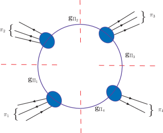
Figure 6: Graphical representation of a quadrupole-cut partitioning of the external legs into an ordered set of four unordered subsets ${\pi_{1},\pi_{2},\pi_{3},\pi_{4}}$ of external particles. The corresponding tree-level diagrams are connected with the propagators of particle $g_{\Pi_{1}},g_{\Pi_{2}},g_{\Pi_{3}},g_{\Pi_{4}}$.

The dimensionality of the parameter vector $\vec{C}_{g_{\Pi_{1}}\cdots g_{\Pi_{k}}}$ depends on the number of denominators. In the case of 5 denominators there is only one parameter, for the terms with 4 denominators we have five parameters, etc. . The parameters are determined by putting sets of denominators to zero and calculating the residue in terms of tree-level amplitudes. Setting denominator factors to zero is on a par with cutting the corresponding propagators as required by generalized $D$-dimensional unitarity. Let $\ell_{\Pi_{1}\cdots\Pi_{c}}$ be the “on-shell” loop momentum fulfilling the “unitarity condition”:

$$d_{g_{\Pi_{1}}}(\ell_{\Pi_{1}\cdots\Pi_{c}})\;=\cdots=\;d_{g_{\Pi_{c}}}(\ell_{\Pi_{1}\cdots\Pi_{c}})\;=0\,;\qquad c=2,\ldots,C_{\rm max}\ .$$ (49)

To fulfill the unitarity conditions we allow also complex values for the components of the loop momenta. The parametric form of the numerator functions for $c$-cuts becomes

$${\cal P}_{c}\left(\vec{C}_{g_{\Pi_{1}}\cdots g_{\Pi_{c}}}\mid\ell_{\Pi_{1}\cdots\Pi_{c}}\right)\;=\;\mbox{Res}_{g_{\Pi_{1}}\cdots g_{\Pi_{c}}}\left({\cal A}^{(1)}\left({\bf f}_{1},\ldots,{\bf f}_{n}\mid\ell_{\Pi_{1}\cdots\Pi_{c}}\right)\right)$$ (50)

$$- \sum_{m=c+1}^{C_{\rm max}}\ \ \sum_{PP_{\widehat{\pi}_{1},\ldots,\widehat{\pi}_{m}}(1,\ldots,n)}\delta_{\Pi_{1}\widehat{\Pi}_{1}}\cdots\delta_{\Pi_{c}\widehat{\Pi}_{c}}\ \sum_{g_{\widehat{\Pi}_{c+1}}\cdots g_{\widehat{\Pi}_{m}}}\ \frac{{\cal P}_{m}\left(\vec{C}_{g_{\widehat{\Pi}_{1}}\cdots g_{\widehat{\Pi}_{m}}}\mid\widehat{\ell}_{\widehat{\Pi}_{1}\cdots\widehat{\Pi}_{c}}\right)}{d_{g_{\widehat{\Pi}_{c+1}}}(\widehat{\ell}_{\widehat{\Pi}_{1}\cdots\widehat{\Pi}_{c}})\cdots d_{g_{\widehat{\Pi}_{m}}}(\widehat{\ell}_{\widehat{\Pi}_{1}\cdots\widehat{\Pi}_{c}})}\ .$$

where the sum $PP_{\widehat{\pi}_{1},\ldots,\widehat{\pi}_{m}}(1,\ldots,n)$ over all $m!$ permutations of the $m$ partitions is supplemented with the $\delta$-functions to generate the appropriate subtraction functions. Each individual subtraction expression has to be evaluated with the appropriate shift of the loop-momentum, $\widehat{\ell}_{\widehat{\Pi}_{1}\cdots\widehat{\Pi}_{c}}$. This equation provides us with an iterative procedure starting with the highest number of cuts. For a given number of cuts, the numerator function becomes the residue of one-loop integrand function minus the known contributions of terms with higher number of denominator factors. The residue of the one-loop integrand factorizes into a product of tree-level amplitudes (see e.g. Fig. 6):

$$\mbox{Res}_{g_{\Pi_{1}}\cdots g_{\Pi_{c}}}\left({\cal A}^{(1)}\left({\bf f}_{1},\ldots,{\bf f}_{n}\mid\ell_{\Pi_{1}\cdots\Pi_{c}}\right)\right) = {\left[d_{g_{\Pi_{1}}}(\ell)\times\cdots\times d_{g_{\Pi_{c}}}(\ell)\times{\cal A}^{(1)}\left({\bf f}_{1},\ldots,{\bf f}_{n}\mid\ell\right)\right]}_{\ell=\ell_{\Pi_{1}\cdots\Pi_{c}}}$$ (51)

$$= \sum_{{\bf g}_{1}\cdots{\bf g}_{c}}\left\{\prod_{k=1}^{c}{\cal M}^{(0)}\big{(}\,{\bf g}_{k}^{\dagger},\,{\bf f}_{\pi_{k}},\,{\bf g}_{k+1}\big{)}\right\}\ ,$$

where the index $k$ is cyclic (i.e. ${\bf g}_{c+1}={\bf g}_{1}$) and ${\bf g}_{k}$ denotes the particles resulting from the cut lines.

We can determine the parametric vector $\vec{C}_{g_{\Pi_{1}}\cdots g_{\Pi_{c}}}$ in Eq. (50) by evaluating the right hand side for a set of loop momenta fulfilling the unitarity constraint of Eq. (49). The only physics model input is given through the tree-level on-shell amplitudes, ${\cal M}^{(0)}$, which we evaluate using Eqs. (6) and (11). Two of the external lines to the on-shell tree-level amplitudes are generated by the $D$-dimensional cut lines. These external states have in general complex, 5-dimensional momenta. This extension of the momenta does not modify the general structure of the tree-level level recursion relations discussed in the previous section. In this way we obtain a fully specified algorithm to determine the parameters and thereby the parametric form on the left hand side of Eq. (46).

It is instructive to illustrate the structure given by Eq. (46) for a simple example. Let us consider the cut-constructible, $D=4$, part of the box terms in 4-gluon scattering ($n=4$, $k=4$). In this case we have no pentagon terms and the numerator functions of the box terms are parametrized by two coefficients

$$\sum_{RP_{1234}(1,2,3,4)}\ \ \sum_{f=\{g,q\}}\ \frac{{\cal P}_{4}\left(\vec{C}_{f_{1}f_{2}f_{3}f_{4}}\mid\ell\right)}{d_{f_{1}}(\ell)d_{f_{12}}(\ell)d_{f_{123}}(\ell)d_{f_{1234}}(\ell)}$$ (52)

$$= \frac{{\cal P}_{4}\left(\vec{C}_{g_{1}g_{2}g_{3}g_{4}}\mid\ell\right)}{d_{g_{1}}(\ell)d_{g_{12}}(\ell)d_{g_{123}}(\ell)d_{g_{1234}}(\ell)}+\frac{{\cal P}_{4}\left(\vec{C}_{g_{1}g_{3}g_{4}g_{2}}\mid\ell\right)}{d_{g_{1}}(\ell)d_{g_{13}}(\ell)d_{g_{134}}(\ell)d_{g_{1342}}(\ell)}+\frac{{\cal P}_{4}\left(\vec{C}_{g_{1}g_{4}g_{2}g_{3}}\mid\ell\right)}{d_{g_{1}}(\ell)d_{g_{14}}(\ell)d_{g_{142}}(\ell)d_{g_{1423}}(\ell)}$$

$$+ \frac{{\cal P}_{4}\left(\vec{C}_{q_{1}q_{2}q_{3}q_{4}}\mid\ell\right)}{d_{q_{1}}(\ell)d_{q_{12}}(\ell)d_{q_{123}}(\ell)d_{q_{1234}}(\ell)}+\frac{{\cal P}_{4}\left(\vec{C}_{q_{1}q_{3}q_{4}q_{2}}\mid\ell\right)}{d_{q_{1}}(\ell)d_{q_{13}}(\ell)d_{q_{134}}(\ell)d_{q_{1342}}(\ell)}+\frac{{\cal P}_{4}\left(\vec{C}_{q_{1}q_{4}q_{2}q_{3}}\mid\ell\right)}{d_{q_{1}}(\ell)d_{q_{14}}(\ell)d_{q_{142}}(\ell)d_{q_{1423}}(\ell)}$$

where

$${\cal P}_{4}\left(\vec{C}_{f_{1}f_{2}f_{3}f_{4}}\mid\ell\right)=C^{(0)}_{f_{1}f_{2}f_{3}f_{4}}+C^{(1)}_{f_{1}f_{2}f_{3}f_{4}}\times\ell{\bf\cdot}n;\ n_{\mu}=\epsilon_{\mu\mu_{1}\mu_{2}\mu_{3}}p_{1}^{\mu_{1}}p_{12}^{\mu_{2}}p_{123}^{\mu_{3}}\ .$$ (53)

The parameters are calculated by using the residue formula of Eq. (51). After the coefficients of the box functions have been obtained, one turns to calculate the coefficients of the triangle contributions. The numerator function for the triangle cut of the quark-loop contribution, Eq. (50), becomes

$${\cal P}_{3}\left(\vec{C}_{q_{1}q_{2}q_{34}}\mid\ell_{\Pi_{1}\Pi_{2}\Pi_{34}}\right) = \mbox{Res}_{q_{1}q_{2}q_{34}}\Big{(}{\cal A}^{(1)}({\bf g}_{1},{\bf g}_{2},{\bf g}_{3},{\bf g}_{4}\mid\ell_{\Pi_{1}\Pi_{2}\Pi_{34}})\Big{)}$$ (54)

$$- \frac{{\cal P}_{4}\left(\vec{C}_{q_{1}q_{2}q_{3}q_{4}}\mid\ell_{\Pi_{1}\Pi_{2}\Pi_{34}}\right)}{d_{q_{123}}(\ell_{\Pi_{1}\Pi_{2}\Pi_{34}})}\;-\;\frac{{\cal P}_{4}\left(\vec{C}_{q_{1}q_{2}q_{4}q_{3}}\mid\ell_{\Pi_{1}\Pi_{2}\Pi_{34}}\right)}{d_{q_{124}}(\ell_{\Pi_{1}\Pi_{2}\Pi_{34}})}\ ,$$

where the residuum of the quark loop can be calculated again using Eq. (51),

$$\mbox{Res}_{q_{1}q_{2}q_{34}}\left({\cal A}^{(1)}({\bf g}_{1},{\bf g}_{2},{\bf g}_{3},{\bf g}_{4}\mid\ell_{\Pi_{1}\Pi_{2}\Pi_{34}})\right) =$$ (55)

$$=\;\left[\,d_{q_{1}}(\ell)\times d_{q_{12}}(\ell)\times d_{q_{1234}}(\ell)\times{\cal A}^{(1)}({\bf g}_{1},{\bf g}_{2},{\bf g}_{3},{\bf g}_{4}\mid\ell)\,\right]_{\ell=\ell_{\Pi_{1}\Pi_{2}\Pi_{34}}}$$

$$=\sum_{{\bf q}_{1}{\bf q}_{2}{\bf q}_{3}}{\cal M}^{(0)}({\bf q}_{1}^{\dagger},{\bf g}_{1},{\bf\bar{q}}_{2})\times{\cal M}^{(0)}({\bf q}_{2}^{\dagger},{\bf g}_{2},{\bf\bar{q}}_{3})\times{\cal M}^{(0)}({\bf q}_{3}^{\dagger},{\bf g}_{3},{\bf g}_{4},{\bf\bar{q}}_{1})\ .$$

Finally, we can obtain the one-loop amplitude, Eq. (45), by integrating out the parametric forms on the right hand side of Eq. (46) over the loop momentum. In this way one finds the master-integral decomposition of the one-loop matrix element for every specified scattering configuration point [10]:

$${\cal M}^{(1)}\left({\bf f}_{1},\ldots,{\bf f}_{n}\right)\;=\int\frac{d^{D}\,\ell}{(2\pi)^{D}}\ {\cal A}^{(1)}\left({\bf f}_{1},\ldots,{\bf f}_{n}\mid\ell\right)$$ (56)

$$= \sum_{k=1}^{C_{\rm max}}\ \sum_{RP_{\pi_{1}\cdots\pi_{k}}(1,2,\ldots,n)}\ \sum_{g_{\Pi_{1}}\cdots g_{\Pi_{k}}}S_{F}^{(g_{\Pi_{1}}\cdots g_{\Pi_{k}})}\times\left(\bar{C}_{g_{\Pi_{1}}\cdots g_{\Pi_{k}}}{\cal I}_{g_{\Pi_{1}}\cdots g_{\Pi_{k}}}+\bar{\bar{C}}_{g_{\Pi_{1}}\cdots g_{\Pi_{k}}}{\cal R}_{g_{\Pi_{1}}\cdots g_{\Pi_{k}}}\right)$$

where $S_{F}^{(g_{\Pi_{1}}\cdots g_{\Pi_{k}})}$ is the loop-integral symmetry factor (e.g. for a gluonic self-energy, the symmetry factor is $\frac{1}{2}$), the ${\cal I}_{g_{\Pi_{1}}\cdots g_{\Pi_{k}}}$ denote the scalar master-integral functions corresponding to the generalized cut given by the ordered partition list $\{\Pi_{1}\cdots\Pi_{k}\}$ and flavors of the cut lines $(g_{\Pi_{1}}\cdots g_{\Pi_{k}})$. The terms ${\cal R}_{g_{\Pi_{1}}\cdots g_{\Pi_{k}}}$ are the leading terms of the higher dimensional scalar integrals in the limit $D\to 4$,

$${\cal R}_{f_{\Pi_{1}}f_{\Pi_{2}}f_{\Pi_{3}}f_{\Pi_{4}}} = -\frac{1}{6}\ ,$$

$${\cal R}_{f_{\Pi_{1}}f_{\Pi_{2}}f_{\Pi_{3}}} = \frac{1}{2}\ ,$$

$${\cal R}_{f_{\Pi_{1}}f_{\Pi_{2}}} = -\frac{\left(K_{\Pi_{1}}-K_{\Pi_{2}}\right)^{2}}{6}+\frac{m_{f_{\Pi_{1}}}^{2}+m_{f_{\Pi_{2}}}^{2}}{2}\ ,$$

$${\cal R}_{f_{\Pi_{1}}} = 0\ .$$ (57)

The scalar master integrals

$${\cal I}_{f_{\Pi_{1}}\cdots f_{\Pi_{k}}}\;=\;I_{k}\left(K_{\Pi_{1}},\ldots,K_{\Pi_{k}},m_{f_{\Pi_{1}}},\ldots,m_{f_{\Pi_{k}}}\right)\ ,$$ (58)

can be evaluated by e.g. using the numerical package developed in Ref. [41]. In Eq. (56) the coefficients $\bar{C}$ and $\bar{\bar{C}}$ are determined by applying Eqs. (50) and (51) using a numerical algorithm. The $\bar{\bar{C}}$ coefficients are generated due to the dimensional regularization procedure and are associated with the higher dimensional terms in the parametric forms.

4.2 Numerical Results for the Virtual Corrections of $n$-gluon Scattering

We have applied the formalism of the previous sections to multi-gluon scattering. To this end we have extended the implementation presented in Ref. [30]. Three major changes are required to alter the generalized-unitarity based algorithm for the evaluation of color-ordered amplitudes to a numerical algorithm capable of calculating color-dressed one-loop amplitudes. First, in the decomposition of the one-loop integrands (cf. Eq. (3) of Ref. [30] and Eq. (46)), all sums over ordered cuts have to be changed into sums over partitions, which include all configurations obtained by non-cyclic and non-reflective permutations:

$$\sum\limits_{[i_{1}|i_{k}]}\quad\to\quad\sum\limits_{{RP}_{\pi_{1}\cdots\pi_{k}}(1\ldots n)}\quad.$$ (59)

Note that $[i_{1}|i_{k}]=1\leq i_{1}<i_{2}<\cdots<i_{k}\leq n$. Second, the tree-level amplitudes occurring in the determination of the integrand’s residues have to be calculated from color-dressed recursion relations. In addition, one not only has to sum over the internal polarizations of the gluons but also over their internal colors when computing these residues. Third, gluon bubble coefficients need to be supplemented by a symmetry factor of $1/2!$. The appearance of the symmetry factor is associated with the parametrization ambiguity of the subtraction terms in the double cuts. For example, Eq. (50) gives for one of the double cuts in 4-gluon scattering

$${\cal P}_{2}(\vec{C}_{g_{12}g_{34}}\mid\ell) = \mbox{Res}_{g_{12}g_{34}}\Big{(}{\cal A}^{(1)}({\bf g}_{1},{\bf g}_{2},{\bf g}_{3},{\bf g}_{4}\mid\ell)\Big{)}$$ (60)

$$- \frac{{\cal P}_{3}(\vec{C}_{g_{1}g_{2}g_{34}}\mid\ell)}{d_{g_{1}}(\ell)}\;-\;\frac{{\cal P}_{3}(\vec{C}_{g_{2}g_{1}g_{34}}\mid\ell)}{d_{g_{2}}(\ell)}\;-\;\frac{{\cal P}_{3}(\vec{C}_{g_{3}g_{4}g_{12}}\mid\ell)}{d_{g_{3}}(\ell)}\;-\;\frac{{\cal P}_{3}(\vec{C}_{g_{4}g_{3}g_{12}}\mid\ell)}{d_{g_{4}}(\ell)}$$

$$- \frac{{\cal P}_{4}(\vec{C}_{g_{1}g_{2}g_{3}g_{4}}\mid\ell)}{d_{g_{1}}(\ell)d_{g_{123}}(\ell)}\;-\;\frac{{\cal P}_{4}(\vec{C}_{g_{2}g_{1}g_{3}g_{4}}\mid\ell)}{d_{g_{2}}(\ell)d_{g_{213}}(\ell)}\;-\;\frac{{\cal P}_{4}(\vec{C}_{g_{1}g_{2}g_{4}g_{3}}\mid\ell)}{d_{g_{1}}(\ell)d_{g_{124}}(\ell)}\;-\;\frac{{\cal P}_{4}(\vec{C}_{g_{2}g_{1}g_{4}g_{3}}\mid\ell)}{d_{g_{2}}(\ell)d_{g_{214}}(\ell)}$$

$$= \mbox{Res}_{g_{12}g_{34}}\Big{(}{\cal A}^{(1)}({\bf g}_{1},{\bf g}_{2},{\bf g}_{3},{\bf g}_{4}\mid\ell)\Big{)}$$

$$- \frac{{\cal P}_{3}(\vec{C}_{g_{1}g_{2}g_{34}}\mid\ell)}{d_{g_{1}}(\ell)}\;-\;\frac{{\cal P}_{3}(\vec{C}_{g_{1}g_{2}g_{34}}\mid-\ell+K_{1}+K_{2})}{d_{g_{1}}(-\ell+K_{1}+K_{2})}$$

$$- \frac{{\cal P}_{3}(\vec{C}_{g_{3}g_{4}g_{12}}\mid\ell)}{d_{g_{3}}(\ell)}\;-\;\frac{{\cal P}_{3}(\vec{C}_{g_{3}g_{4}g_{12}}\mid-\ell+K_{3}+K_{4})}{d_{g_{3}}(-\ell+K_{3}+K_{4})}$$

$$- \frac{{\cal P}_{4}(\vec{C}_{g_{1}g_{2}g_{3}g_{4}}\mid\ell)}{d_{g_{1}}(\ell)d_{g_{123}}(\ell)}\;-\;\frac{{\cal P}_{4}(\vec{C}_{g_{1}g_{2}g_{3}g_{4}}\mid-\ell+K_{1}+K_{2})}{d_{g_{1}}(-\ell+K_{1}+K_{2})d_{g_{123}}(-\ell+K_{1}+K_{2})}$$

$$- \frac{{\cal P}_{4}(\vec{C}_{g_{1}g_{2}g_{4}g_{3}}\mid\ell)}{d_{g_{1}}(\ell)d_{g_{124}}(\ell)}\;-\;\frac{{\cal P}_{4}(\vec{C}_{g_{1}g_{2}g_{4}g_{3}}\mid-\ell+K_{3}+K_{4})}{d_{g_{1}}(-\ell+K_{3}+K_{4})d_{g_{124}}(-\ell+K_{3}+K_{4})}\ .$$

We see that each of the four possible parametrized terms is subtracted twice with a different choice of the loop momentum. The symmetry factor of $1/2!$ “averages” over the double subtractions.

The results of the new formalism can be tested thoroughly beyond applying the usual consistency checks such as solving for the master-integral coefficients with two independent sets of loop momenta. The value of the double pole (dp) can be cross-checked against the analytic result

$${\cal M}^{(1)}_{\rm dp,th}\;=\;-\,\frac{c_{\Gamma}}{\epsilon^{2}}\,n\,N_{\rm C}\,{\cal M}^{(0)}\ .$$ (61)

Moreover, for a given phase-space point, we can use the ordered algorithm of Ref. [30] to compute the full one-loop amplitude of a certain color and helicity (polarization) configuration. Following the color-decomposition approach, we can analytically calculate the necessary color factors and sum up all relevant orderings to obtain the full result. In particular, we have employed:

$${\cal M}^{(1)}({\bf g}_{1},\ldots,{\bf g}_{n})\;=\sum_{P(2\cdots n)}{A^{(1)}}^{i_{1}\cdots i_{n}}_{j_{1}\cdots j_{n}}(g_{1}^{\lambda_{1}},\ldots,g_{n}^{\lambda_{n}})$$ (62)

$$= \sum_{P(1\cdots n-1)}\left[N_{\rm C}\,\Delta_{1\cdots n}+\sum_{k=1}^{{\rm int}(n/2)}\sum_{m_{1}=1}^{n-k+1}\cdots\sum_{m_{k}=m_{k-1}+1}^{n}(-1)^{k}\Delta_{m_{1}\cdots m_{k}}\Delta_{1\cdots/m_{1}\cdots/m_{k}\cdots n}\right]m^{(1)}(12\cdots n)$$

where

$$\Delta_{12\cdots n}\;=\;\delta^{i_{1}}_{j_{2}}\delta^{i_{2}}_{j_{3}}\cdots\delta^{i_{n-1}}_{j_{n}}\delta^{i_{n}}_{j_{1}}\ .$$ (63)

For example,

$${\cal M}^{(1)}({\bf g}_{1},{\bf g}_{2},{\bf g}_{3},{\bf g}_{4},{\bf g}_{5}) = \sum_{P(2345)}{A^{(1)}}({\bf g}_{1},{\bf g}_{2},{\bf g}_{3},{\bf g}_{4},{\bf g}_{5})$$ (64)

$$= \sum_{P(2345)}\Big{(}N_{c}\,\Delta_{12345}-\Delta_{1}\Delta_{2345}-\Delta_{2}\Delta_{1345}-\Delta_{3}\Delta_{1245}-\Delta_{4}\Delta_{1235}-\Delta_{5}\Delta_{1234}$$

$$\phantom{\sum_{P(2345)}}+\Delta_{12}\Delta_{345}+\Delta_{13}\Delta_{245}+\Delta_{14}\Delta_{235}+\Delta_{15}\Delta_{234}+\Delta_{23}\Delta_{145}+\Delta_{24}\Delta_{135}$$

$$\phantom{\sum_{P(2345)}}+\Delta_{25}\Delta_{134}+\Delta_{34}\Delta_{125}+\Delta_{35}\Delta_{124}+\Delta_{45}\Delta_{123}\Big{)}\,m^{(1)}(12345)\ .$$

Compared to the LO color-ordered decomposition, Eq. (27), the NLO color-ordered decomposition leads to many subleading color factors. The number of one-loop ordered amplitudes with zero color weight is significantly smaller than the corresponding number for tree-level ordered amplitudes. As a result, the advantages of color dressing become more apparent at the one-loop level.

Ordered cuts.
#	5-gon	box	triangle	bubble	sum	${\rm sum}_{n}$	total $=$ sum $\times$	#orderings	${\cal N}_{(ab)_{k}}=$	${\cal N}_{(cd)_{k}}$
$n$	cuts	cuts	cuts	cuts		$\overline{{\rm sum}_{n-1}\!\!}$	#orderings	$=(n-1)!/2$	$(n-2)!$
4	0	1	4	6	11		33	3	2	3
5	1	5	10	10	26	2.36	312	12	6	7
6	6	15	20	15	56	2.15	3,360	60	24	22
7	21	35	35	21	112	2.00	40,320	360	120	40
8	56	70	56	28	210	1.88	529,200	2,520	720	144
9	126	126	84	36	372	1.77	7,499,520	20,160	5,040	756
10	252	210	120	45	627	1.69	113,762,880	181,440	40,320	2,688
11	462	330	165	55	1012	1.61	1,836,172,800	1,814,400	362,880
12	792	495	220	66	1573	1.55	31,394,563,200	19,958,400	3,628,800

Table 3: The number of cuts required for the calculation of one ordered $n$-gluon amplitude. The column labelled “total” gives the number of cuts when calculating all $(n-1)!/2$ ordered amplitudes needed to reconstruct the full virtual correction. The last two columns list the number of non-zero color-weight orderings for two special color configurations given in the text.

Unordered cuts.
#	pentagon	box	triangle	bubble	sum	${\rm sum}_{n}$	ordr total/unordr total
$n$	cuts	cuts	cuts	cuts	$\equiv$ total	$\overline{{\rm sum}_{n-1}\!\!}$	orderings	$(ab)_{k}$	$(cd)_{k}$
4	0	3	6	3	12		2.750	1.833	2.750
5	12	30	25	10	77	6.42	4.052	2.026	2.364
6	180	195	90	25	490	6.36	6.857	2.743	2.514
7	1,680	1,050	301	56	3,087	6.30	13.06	4.354	1.451
8	12,600	5,103	966	119	18,788	6.09	28.17	8.048	1.610
9	83,412	23,310	3,025	246	109,993	5.85	68.18	17.05	2.557
10	510,300	102,315	9,330	501	622,446	5.66	182.8	40.61	2.708
11	2,960,760	437,250	28,501	1,012	3,427,523	5.51	535.7	107.1
12	16,552,800	1,834,503	86,526	2,035	18,475,864	5.39	1699	308.9

Table 4: The number of cuts needed to calculate color-dressed $n$-gluon amplitudes. The last three columns give ratios of total numbers of cuts required to compute the virtual corrections in both the color-decomposition and color-dressed approaches. The first of these columns shows the ratios for all generic color orderings whereas the other columns show the ratios for two specific configurations as given in the text.

For a more quantitative understanding of the one-loop amplitude decomposition, we respectively itemize in Tables 3 and 4 how many cuts need be applied to decompose the color-ordered and color-dressed one-loop integrands for $n$ external gluons. In both cases we separately list the numbers of pentagon, box, triangle and bubble cuts and their sum. While for the ordered cuts these numbers are ruled by combinatorics: ${\cal C}(n,m)=\left({n\atop m}\right)$ with $m=1,\ldots,5$; in the unordered case they are given by the Stirling numbers of the second kind, ${\cal S}_{2}(n,m)$, and therefore grow more quickly with $n$ than those of the ordered cuts. This is exemplified in the “${\rm sum}_{n}/{\rm sum}_{n-1}$” columns of the two tables. The growth factors slowly decrease for larger $n$, approaching the limit of $5$ for the color-dressed case. As emphasized in Table 4 the pentagon-cut calculations dominate in this case over all other cut evaluations. The large-$n$ growth of the total cut number is hence described by that of ${\cal S}_{2}(n,5)$ leading to the observed large-$n$ scaling of $5^{n}$. Using the color-decomposition approach, we have to deal with much fewer cuts per ordering. However, the total number of ordered cuts is obtained only after multiplying with the relevant number of orderings. When considering all possible $(n-1)!/2$ orderings, the final numbers are given in column “total” of Table 3. The last three columns show the number of generic orderings and the numbers $\cal N$ of non-vanishing orderings (i.e. those having non-zero color factors) for two color configurations $(ab)_{k}\equiv(13)(31)(11)\ldots(11)$ and $(cd)_{k}\equiv(22)(12)(23)(31)(11)(22)(33)(11)(22)\ldots\$. Of course, for a fair comparison between the ordered and dressed approach, the latter two columns are of higher interest, since zero color weights are not counted. Still, the ratios of total numbers of ordered versus unordered cuts is always larger than one as can be read off the last three columns of Table 4. Keeping in mind the greater cost of evaluating dressed recursion relations, the color-decomposition approach can be expected to outperform the dressed method as long as these ratios remain of order ${\cal O}(1)$. This in particular is true for simple color configurations such as $(cd)_{k}$.

The analytic knowledge of ${\cal M}^{(1)}({\bf g}_{1},\ldots,{\bf g}_{n})$ presented in Eq. (62) enables us to perform stringent tests of our algorithm and its implementation. We consider $2\to n-2$ processes where the gluons have possible polarization states $\lambda_{k}\in\{+,-\}$ and colors $(ij)_{k}$ where $i_{k},j_{k}\in\{1,2,3\}$ and $k=1,\ldots,n$, i.e. we make use of the color-flow notation. Our $n$-gluon results are given in the 4-dimensional helicity (FDH) scheme [40]. In almost all cases, we compare our new method labelled by “drss” with the color-decomposition approach, which – since it makes use of the ordered algorithm – we denote “ordr”. We will present all our results for two choices of loop-momentum and spin-polarization dimensionalities $D$ and $D_{s}$: the “4D-case” is obtained by setting $D=D_{s}=4$ and sufficient when merely calculating the cut-constructible part (ccp) of the one-loop amplitude. The “5D-case” specified by $D=D_{s}=5$ allows us to determine the complete result (all) including the rational part. In NLO calculations one identifies the momenta of the external gluons with those of well separated jets. We therefore apply cuts on the generated $k=1,\ldots,n$ phase-space momenta ($l=3,\ldots,n$):

$$|\eta_{l}|\;<\;2\,,\qquad p_{\perp,l}\;>\;0.1\,|E_{1}+E_{2}|\,,\qquad\Delta R_{kl}\;>\;0.7\,,$$ (65)

where $\eta_{l}$ and $p_{\perp,l}$ respectively denote the pseudo-rapidity and transverse momentum of the $l$-th outgoing gluon; $\Delta R_{kl}$ describe the pairwise geometric separations in pseudo-rapidity and azimuthal-angle space of gluons $k$ and $l$. We perform a series of studies in the context of double-precision computations: we investigate the accuracies with which the double pole, single pole (sp) and finite part (fp) of the full one-loop amplitudes are determined by our algorithm. We also examine the efficiency of calculating virtual corrections by means of simple phase-space integrations. To begin with, we will verify the expected exponential scaling of the computation time for different numbers of external gluons.

	4D-case							5D-case
$n$	ordr			drss			$\underline{\rm ordr}$	ordr			drss			$\underline{\rm ordr}$
	$\tau^{({\rm a})}_{n}$	$\tau^{({\rm b})}_{n}$	$r_{n}$	$\tau^{({\rm a})}_{n}$	$\tau^{({\rm b})}_{n}$	$r_{n}$	drss	$\tau^{({\rm a})}_{n}$	$\tau^{({\rm b})}_{n}$	$r_{n}$	$\tau^{({\rm a})}_{n}$	$\tau^{({\rm b})}_{n}$	$r_{n}$	drss
4	0.027	0.026		0.061	0.062		0.43	0.053	0.052		0.139	0.140		0.38
5	0.159	0.161	6.04	0.368	0.364	5.95	0.44	0.415	0.412	7.88	1.026	1.029	7.37	0.40
6	1.234	1.235	7.72	2.152	2.146	5.87	0.57	3.887	3.928	9.45	7.137	7.124	6.94	0.55
7	12.07	12.00	9.75	13.06	13.08	6.08	0.92	41.66	41.61	10.7	49.62	49.85	6.98	0.84
8	131.2	131.3	10.9	80.22	80.53	6.15	1.6	493.2	498.6	11.9	348.0	346.9	6.99	1.4
9	1579	1563	12.0	511.6	507.8	6.34	3.1	6316	6296	12.7	2466	2470	7.10	2.6
10	20900	20480	13.2	3640	3629	7.13	5.7	88320	88810	14.0	21590	21620	8.75	4.1

Table 5: Computer times $\tau_{n}$ in seconds obtained from the 4- and 5-dimensional evaluation of $n$-gluon virtual corrections at two random phase-space points $\rm a$ and $\rm b$ using a 3.00 GHz Intel Core2 Duo processor. The results are shown for both the color-ordered and color-dressed method. All virtual corrections were evaluated twice to check for the consistency of the solutions. The $n$ gluons have colors $(ab)_{k}$ and polarizations $\kappa_{k}$ as specified in the text. Also given are the ratios $r_{n}=\tau_{n}/\tau_{n-1}$ where $\tau_{n}$ is the time to compute the correction for $n$ gluons, in particular $\tau_{n}=(\tau^{({\rm a})}_{n}+\tau^{({\rm b})}_{n})/2$. The $\tau_{n}$ ratios of the ordered versus dressed method are depicted in the respective last column of the 4- and 5-dimensional case.

	4D-case						5D-case						4D/5D
$n$	ordr			drss			ordr			drss			ordr	drss
	$\tau^{({\rm a})}_{n}$	$\tau^{({\rm b})}_{n}$	$r_{n}$	$\tau^{({\rm a})}_{n}$	$\tau^{({\rm b})}_{n}$	$r_{n}$	$\tau^{({\rm a})}_{n}$	$\tau^{({\rm b})}_{n}$	$r_{n}$	$\tau^{({\rm a})}_{n}$	$\tau^{({\rm b})}_{n}$	$r_{n}$
4	0.030	0.030		0.069	0.070		0.059	0.059		0.156	0.157		0.51	0.44
5	0.180	0.179	5.98	0.418	0.413	5.98	0.464	0.465	7.87	1.150	1.148	7.34	0.39	0.36
6	1.384	1.383	7.71	2.419	2.410	5.81	4.370	4.340	9.38	8.036	7.996	6.98	0.32	0.30
7	13.53	13.52	9.78	14.64	14.65	6.07	46.65	46.40	10.7	56.06	55.99	6.99	0.29	0.26
8	147.2	147.5	10.9	90.48	91.60	6.22	550.9	549.5	11.8	395.2	391.9	7.02	0.27	0.23
9	1766	1764	12.0	585.9	585.0	6.43	7013	7029	12.8	2844	2845	7.23	0.25	0.21
10	23100	22830	13.0	4233	4208	7.21	98760	98360	14.0	24220	24410	8.55	0.23	0.17

Table 6: Computer times $\tau_{n}$ in seconds for the same settings as used in Table 5, this time using a 2.66 GHz Intel Core2 Quad processor. The rightmost part of the table depicts the ratios of 4- versus 5-dimensional computer times for both approaches.

The scaling of the computer time can roughly be estimated by $(f\times C_{\rm max})^{n}$. The constants $C_{\rm max}=5\,(4)$ and $1<f\leq 4$ express the fact that the number of pentagon (box) cuts and the exponential scaling with $n$ of the tree-level color-dressed recursion relation respectively govern the asymptotic scaling behavior of the unordered algorithm. Although one naively expects $f=4$, this factor is reduced by the efficient re-use of gluon currents between different cuts. The $C_{\rm max}^{n}$ growth of the number of cuts reflects the large-$n$ limit of the Stirling number ${\cal S}_{2}(n,C_{\rm max})$. We show four tables summarizing our results for the computation times $\tau_{n}$ of obtaining ${\cal M}^{(1)}({\bf g}_{1},\ldots,{\bf g}_{n})={\cal M}_{n}^{(1)}(\lambda_{k},(ij)_{k})$ by using two independent solutions of the unitarity constraints. The time for the re-computation has been included in $\tau_{n}$. In real applications such a consistency check will become unnecessary, thereby halving the evaluation time per phase-space point. Table 5 lists the times obtained by running the 4- and 5-dimensional algorithms for the calculation of two random phase-space points labelled “$\rm a$” and “$\rm b$”. The $n$ gluons have colors $(ij)_{k}=(ab)_{k}$ and alternating polarizations $\lambda_{k}=\kappa_{k}\equiv+-\ldots+-(+)$. Owing to the absence of pentagon cuts we find that the “4D-case” calculations are faster. More importantly, the computation time does not vary when the $n$-gluon kinematics changes. Hence, we can calculate the ratios $r_{n}=\tau_{n}/\tau_{n-1}$ by defining $\tau_{n}=(\tau^{({\rm a})}_{n}+\tau^{({\rm b})}_{n})/2$ and show these ratios in the table. While for the dressed algorithm these ratios are almost stable, they are larger and increase gradually for the method based on ordered amplitudes. This reflects the $(n-2)!$ factorial growth of the number of non-vanishing orderings of the color configuration $(ab)_{k}$ as given in Table 3. For the dressed approach, we find constant ratios of $r_{n}\approx 6$ and $r_{n}\approx 7$ in the “4D-case” and “5D-case”, respectively. This manifestly confirms our expectation of exponential scaling. The difference between the 4- and 5-dimensional ratios obviously arises because of the absence of pentagon cuts in the “4D-case”. The $r_{10}$ ratios do not fit the constant trend. We cannot exclude though that this is a consequence of the occurrence of large structures of maps to store the vast number of color-dressed coefficients. The increasing number of higher-cut subtractions terms may also cause deviations from the expected scaling, which we derived from our simple arguments stated above. Also, the conceptually easier way of storing all coefficients and calculating the largest-$m$ cuts first is by far not the most economic in terms of memory consumption. For small $n$, the lower complexity of the ordered recurrence relation facilitates a faster calculation of the virtual corrections through ordered amplitudes. The turnaround appears for $7<n<8$ and is just slightly above $n=7$ for the “4D-case”. With $n\geq 8$ the dressed method becomes superior owing to the different growth characteristics of the two approaches. This is neatly expressed by the “ordr/drss” ratios given in Table 5.

We have cross-checked the measured computation times in a different processor environment using exactly the same settings. The results are shown in Table 6 and consistent with those of Table 5. Instead of the “ordr/drss” ratios, here we list ratios comparing the 4- and 5-dimensional computation for both approaches. They stress the relative importance of the pentagon-cut evaluations, which start to dominate the full calculation when $n$ gets large.

	4D-case							5D-case
$n$	ordr			drss			$\underline{\rm ordr}$	ordr			drss			$\underline{\rm ordr}$
	$\tau^{(\sigma_{k})}_{n}$	$\tau^{(\kappa_{k})}_{n}$	$r_{n}$	$\tau^{(\sigma_{k})}_{n}$	$\tau^{(\kappa_{k})}_{n}$	$r_{n}$	drss	$\tau^{(\sigma_{k})}_{n}$	$\tau^{(\kappa_{k})}_{n}$	$r_{n}$	$\tau^{(\sigma_{k})}_{n}$	$\tau^{(\kappa_{k})}_{n}$	$r_{n}$	drss
4	0.049	0.045		0.074	0.076		0.63	0.088	0.085		0.153	0.155		0.56
5	0.186	0.185	3.95	0.364	0.364	4.85	0.51	0.479	0.483	5.56	1.000	1.000	6.49	0.48
6	1.186	1.182	6.38	2.071	2.068	5.69	0.57	3.629	3.586	7.50	6.805	6.752	6.78	0.53
7	4.185	4.277	3.57	11.82	11.77	5.70	0.36	14.02	13.95	3.88	44.42	44.46	6.56	0.31
8	27.12	26.96	6.39	70.34	71.10	6.00	0.38	98.52	99.13	7.07	294.8	297.8	6.67	0.33
9	245.0	242.9	9.02	443.8	445.5	6.29	0.55	960.3	954.8	9.69	2080	2070	7.00	0.46
10	1442	1446	5.92	3265	3270	7.35	0.44	5943	5968	6.22	18610	18480	8.94	0.32
11				28670	28690	8.78
6				2.044		5.62
7				11.66		5.70
8				68.85		5.90
9				420.4		6.11
10				2972		7.07
11				26310		8.85
12					292000	11.1

Table 7: Computer times $\tau_{n}$ in seconds obtained for the color-ordered and color-dressed evaluation of $n$-gluon virtual corrections in 4 and 5 dimensions using a 3.00 GHz Intel Core2 Duo processor. Results are shown for two different polarization choices $\sigma_{k}$ and $\kappa_{k}$. The virtual corrections were computed at the same random phase-space point with the $n$-gluon colors set to $(cd)_{k}$. The choices are specified in the text. Ratios $r_{n}=\tau_{n}/\tau_{n-1}$ are given where $\tau_{n}=(\tau^{(\sigma_{k})}_{n}+\tau^{(\kappa_{k})}_{n})/2$ is the time to evaluate the correction for $n$ gluons two times. The re-computation is used to check both solutions for their consistency. The $\tau_{n}$ ratios of the ordered versus dressed method are depicted in the respective last column of the 4- and 5-dimensional case.

	4D-case					5D-case					4D/5D
$n$	ordr		drss		$\underline{\rm ordr}$	ordr		drss		$\underline{\rm ordr}$	ordr	drss
	$\tau_{n}$	$r_{n}$	$\tau_{n}$	$r_{n}$	drss	$\tau_{n}$	$r_{n}$	$\tau_{n}$	$r_{n}$	drss
4	0.026		0.062		0.42	0.065		0.151		0.43	0.40	0.41
5	0.222	8.54	0.394	6.35	0.56	0.615	9.46	1.139	7.54	0.54	0.36	0.35
6	1.863	8.39	2.378	6.04	0.78	5.544	9.01	7.970	7.00	0.70	0.33	0.30
7	15.06	8.08	14.58	6.13	1.03	50.41	9.09	56.94	7.14	0.89	0.30	0.26
8	129.2	8.58	93.09	6.38	1.39	476.7	9.46	401.5	7.05	1.19	0.27	0.23
9	1127	8.72	603.6	6.48	1.87	4483	9.40	2800	6.97	1.60	0.25	0.22
10	10980	9.74	3961	6.56	2.77	50260	11.2	25140	8.98	2.00	0.22	0.16

Table 8: Color-configuration averaged computation times $\tau_{n}$ in seconds obtained from the 4- and 5- dimensional color-ordered and color-dressed evaluations of $n$-gluon virtual corrections using 2.66 GHz Intel Core2 Quad processors. Results are shown for random phase- and color-space points and alternating gluon polarizations $\lambda_{k}=\kappa_{k}$, see text. The respective growth factors $r_{n}=\tau_{n}/\tau_{n-1}$ are given where $\tau_{n}$ denotes the time that is needed to calculate the $n$-gluon one-loop amplitude two times. The re-computation is used to check the two solutions for their consistency. Several time ratios are formed to compare the ordered with the dressed method and the 4- with the 5-dimensional computation. These ratios are displayed in the columns indicated accordingly.

In Table 7 we detail computation times when varying the polarizations of the $n$ gluons while keeping their color configuration fixed. We have chosen the two settings $\lambda_{k}=\sigma_{k}\equiv++-\ldots-$ and, as before, $\lambda_{k}=\kappa_{k}$. In terms of colors we consider the computationally less involved point $(ij)_{k}=(cd)_{k}$. Both amplitudes are calculated at the same random phase-space point “$\rm c$” dissimilar from previous points “${\rm a}$” and “${\rm b}$”. For none of our four calculational options, we notice manifest deviations between the times $\tau^{(\lambda_{k})}_{n}$ associated with the two polarization settings. When inspecting the “ordr/drss” ratios, we observe that the ordered approach is advantageous in cases where only a few orderings contribute to the result of a certain point in color space. The fluctuations seen in the growth factors mirror the unsteady increase with $n$ in non-zero orderings depicted in the last column of Table 3. For the dressed approach, we get similar, though somewhat smaller, growth factors compared to the previous test. In order to validate the dressed algorithm up to $n=12$ external gluons, we introduced a few more optimizations specific to the 4-dimensional calculations. The lower part of Table 7 shows the computer times, which we obtained after optimization. They are consistent with our previous findings. As mentioned before, $r_{n\geq 10}>6$ likely occur for reasons of increasingly complex higher-cut subtractions and computer limitations in dealing with large memory structures.

configuration:	hard colors $(ab)_{k}$		simple colors $(cd)_{k}$		random non-zero colors
fit values:	$a/10^{-6}$sec	$b$	$a/10^{-6}$sec	$b$	$a/10^{-6}$sec	$b$
4D, ordr	1.91	$9.75\ ^{+0.59}_{-0.56}$	34.5	$5.65\ ^{+0.32}_{-0.30}$	4.67	$8.57\ ^{+0.10}_{-0.09}$
5D, ordr	2.66	$10.99\ ^{+0.48}_{-0.46}$	45.6	$6.39\ ^{+0.29}_{-0.28}$	7.84	$9.46\ ^{+0.13}_{-0.12}$
4D, drss	39.4	$6.19\ ^{+0.09}_{-0.08}$	28.2	$6.51\ ^{+0.29}_{-0.28}$	38.7	$6.30\ ^{+0.04}_{-0.04}$
5D, drss	50.8	$7.21\ ^{+0.10}_{-0.10}$	62.5	$6.92\ ^{+0.08}_{-0.09}$	53.3	$7.28\ ^{+0.11}_{-0.09}$

Table 9: Parameter values $a$ and $b$ obtained from curve fitting of the computation times $\tau_{n}$ to the functional form of $\tau_{n}=a\,b^{n}$. The results are given for the three different $n$-gluon color assignments used in Tables 5 (hard), 7 (simple) and 8 (random) and for all four algorithms the 4- and 5-dimensional color-ordered and color-dressed algorithm.

For the calculation of the virtual corrections, one might question whether there exist enough points in color space that occur with many trivial orderings. If so, the color-decomposition based method would be more efficient on average. This is not the case for larger $n$ as shown in Table 8. For gluon multiplicities of $n=4,\ldots,10$ and polarizations set according to $\kappa_{k}$, we list mean computation times, growth factors, “ordr/drss” and “4D/5D” ratios obtained for one-loop amplitude evaluations where the phase- and color-space points have been chosen randomly. Following the method outlined in Section 3.3, we only considered non-zero color configurations. We averaged over many events, for $n=4,\ldots,10$ gluons, we used ${\cal O}(10^{6}),\ldots,{\cal O}(10^{2})$ points. We observe that the pattern of the results in Table 8 resembles that found in Tables 5 and 6 where we have studied the more complicated color point $(ik)_{k}=(ab)_{k}$. The ratios comparing the ordered and dressed approach are smaller with respect to those of Tables 5 and 6. This signals that the mean number of contributing orderings is somewhat lower than for the $(ab)_{k}$ case. We finally report dressed growth factors that are consistent with our previous findings confirming the approximate $6^{n}$ and $7^{n}$ growths in computational complexity of the new method for the 4- and 5-dimensional case, respectively.

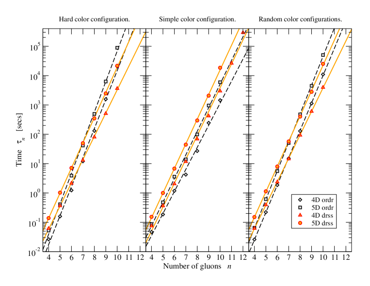
Figure 7: Computation times $\tau_{n}$ versus the number $n$ of external gluons for the three different gluon color assignments used in Tables 5 (hard), 7 (simple) and 8 (random). The results reported in these tables are shown for the 4- and 5-dimensional color-ordered and -dressed algorithms. The solid and dashed curves each represent the outcomes of the fits listed in Table 9 for both the dressed and ordered approach, respectively.

Using the results of Tables 5, 7 and 8 we have performed fits to the functional form $\tau_{n}=a\,b^{n}$. We show the outcome of the curve fittings in Table 9. Recall that the computation times have been obtained by using different color assignments for the $n$ gluons. Tables 5 and 7 present results where we have chosen $(ij)_{k}=(ab)_{k}$ and $(ij)_{k}=(cd)_{k}$ as examples of hard and simple color configurations, respectively. We have averaged over non-zero color settings to find the results of Table 8. Considering the performance of the dressed algorithm, we conclude that these data are in agreement with exponential growth for all color assignments. The errors on the fit parameter $b$ are relatively small, only the 4-dimensional case of simple colors is somewhat worse because we included results up to $n=12$ where parts of the computation become less efficient as explained above. The hard- and simple-colors case of the ordered approach show rather large errors for the $b$-parameter signalling that the genuine scaling law is not of an exponential kind in both cases. Interestingly, one observes an effective exponential scaling when averaging over many non-zero color configurations. The growth described by the $b$-parameter is however a good two units stronger for the ordered approach than the growth seen in the color-dressed approach. To summarize, we have plotted in Fig. 7 all computer times reported in Tables 5, 7 and 8 as a function of the number of external gluons in the range $4\leq n\leq 12$. We have included in these plots the curves $\tau_{n}=a\,b^{n}$, which we calculated from the respective fit parameters stated in Table 9.

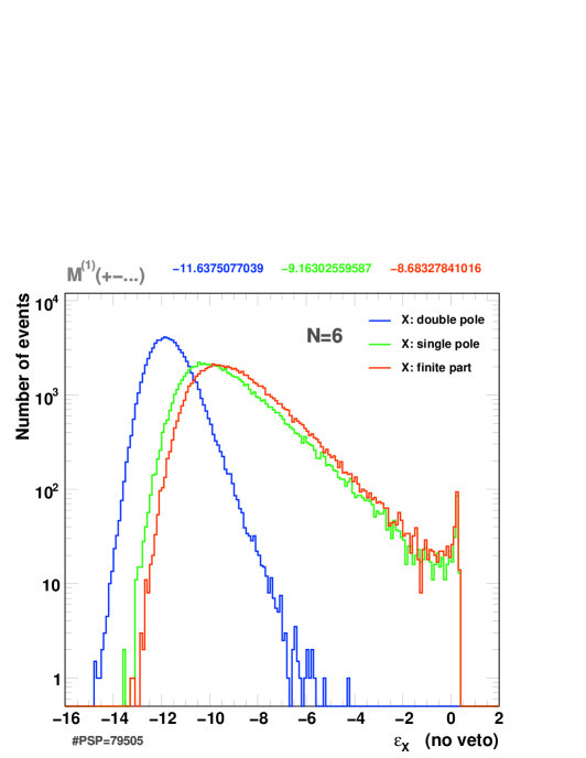
Figure 8: Relative accuracies of the $1/\epsilon^{2,1,0}$ poles of $n=6$ gluon one-loop amplitudes as determined by the double-precision color-dressed algorithm. The gluon polarizations are given by $\lambda_{k}=+-+-+-$, colors were chosen randomly among non-zero configurations. Vetoed events are included, only those with unstable ortho-vectors are left out, see text for more explanations. The mean accuracies and the number of randomly picked phase-space points are displayed in the top row and bottom left corner of the plot, respectively.

In the following we will discuss the quality of the semi-numerical evaluations of ${\cal M}_{n}^{(1)}$ amplitudes for both the color-ordered and color-dressed approaches. To this end we analyze the logarithmic relative deviations of the double pole, single pole and finite part. Independent of the number $n$ of gluons, we define them as follows:

$$\varepsilon_{\rm dp}\;=\;\log_{10}\,\frac{|{\cal M}^{(1)[1]}_{\rm dp,num}-{\cal M}^{(1)}_{\rm dp,th}|}{|{\cal M}^{(1)}_{\rm dp,th}|}\,,\qquad\varepsilon_{\rm s/fp}\;=\;\log_{10}\,\frac{2\,|{\cal M}^{(1)[1]}_{\rm s/fp,num}-{\cal M}^{(1)[2]}_{\rm s/fp,num}|}{|{\cal M}^{(1)[1]}_{\rm s/fp,num}|+|{\cal M}^{(1)[2]}_{\rm s/fp,num}|}\ ,$$ (66)

where the structure of the double-poles ${\cal M}^{(1)}_{\rm dp,th}$ is known analytically given by Eq. (61). We use two independent solutions denoted by $[1]$ and $[2]$ to test the accuracy of the single poles and finite parts. All results reported here were obtained by using double-precision computations. We have run all our algorithms by choosing color configurations and phase-space points at random. Colors are distributed according to the “Non-Zero” method presented in Sec. 3.3. The phase-space points are accepted only if they obey the cuts, which we have specified at the beginning of this subsection. The gluon polarizations are always alternating set by $\lambda_{k}=\kappa_{k}$. Figure 8 shows the $\varepsilon$ distributions in absolute normalization, which we obtain from the 5-dimensional color-dressed calculation for the case of $n=6$ external gluons. The number of points used to generate the plots is given in the bottom left corner, the top rows display the means of the double-, single-pole and finite-part distributions. Limited to double-precision computations, we find that the numerical accuracy of our results for ${\cal M}_{n}^{(1)}$ is satisfying. With $\varepsilon$ peak positions smaller than the respective mean values $\langle\varepsilon_{\rm d/s/fp}\rangle<-8$, we are able to provide sufficiently accurate solutions for almost all phase-space configurations. There is however a certain fraction of events where the single pole and finite part cannot be determined reliably. These ${\cal O}(100)$ events occur because in exceptional cases small denominators, such as vanishing Gram determinants made of external momenta, cannot be completely avoided by the generalized-unitarity algorithms. We also see accumulation effects where larger numbers get multiplied together while determining the subtraction of higher-cut contributions. Owing to the limited range of double-precision calculations, such effects can lead to insufficient cancellations of intermediate large numbers that are supposed to cancel out eventually. The current implementation of the algorithm has no special treatment for these exceptional events. One either has to come up with a more sophisticated method treating these points separately or increase the precision with which the corrections are calculated. Both of which is beyond the scope of this paper and we leave it at vetoing these points. Yet, we need robust criteria that allow us to keep track of the quality of our solutions: we first test the orthonormal basis vectors that span the space complementary to the physical space constructed from the external momenta associated with the particular cut configuration under consideration. Failures in generating these basis vectors always lead to the rejection of the event. In the example of Fig. 8, such events occurred with a rate of $0.6\%$ and were not included in the plot. Secondly, and more importantly, we test the reliability of solving the systems of equations to determine the master-integral coefficients. To this end we generate an extra 4-dimensional loop momentum during the evaluation of the bubble coefficients establishing the cut-constructible part. Inaccuracies in solving for triangle etc. coefficients will be also detected, since at this level all higher-cut subtractions are necessary to obtain the correct value of the bubble coefficients. We use the extra loop momentum to individually re-solve for the cut-constructible bubble coefficient and compare this solution with the one obtained in first place. We veto the event, if the deviation $\Delta_{\rm veto}$ in the complex plane of the two solutions exceeds a certain amount. We fix the veto cut at $\Delta_{\rm veto}=0.02$ for this publication. Having this cross-check at hand, we gain nice control over the events populating the tail of the accuracy distributions in Fig. 8. Applying the veto, we arrive at the distributions presented in the top left plot of Fig. 11 where the steeper tails clearly demonstrate the effect of the veto. Certainly, both these shortcomings of imprecise ortho-vectors and inaccurately solved coefficients can be lifted by switching to higher precision whenever the respective double-precision evaluations have not passed our criteria. Accordingly, Table 10 quantifies the fractions of events, which are within the scope of the color-dressed and color-ordered algorithms presented here. Owing to the more complicated event structures, the fraction of rejected events increases with $n$, where most of the events fail the bubble-coefficient test. We observe that the loss of events is more severe for the ordered algorithm.

$n\;$	4D, ordr	5D, ordr	4D, drss	5D, drss
4	1.0	1.0	1.0	1.0
5	0.992	0.991	0.984	0.984 (0.999)
6	0.960	0.960	0.964	0.972 (0.994)
7	0.872	0.873	0.891	0.892 (0.982)
8	0.635	0.642	0.829	0.825 (0.953)
9	0.182 (0.84)	0.205 (0.81)	0.532 (0.93)	0.533 (0.903)
10	0.000 (0.61)	0.000 (0.50)	0.380 (0.86)	0.330 (0.83)

Table 10: Fractions of $n$-gluon events that have a stable set of basis vectors in orthogonal space and also pass the veto on inaccurate master-integral bubble coefficients when using $\Delta_{\rm veto}=0.02$. In brackets, fractions of $n$-gluon events that pass the test for unstable ortho-vectors.

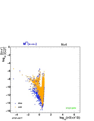
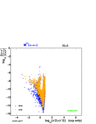
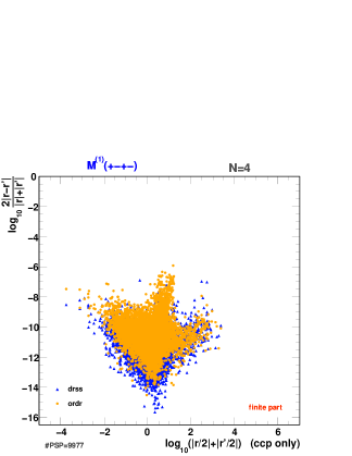
Figure 9: Double-, single-pole and finite-part accuracy distributions (upper part) and scatter graphs (lower part) extracted from double-precision computations of one-loop amplitudes for $n={\tt N}=4$ gluons with polarizations $\lambda_{k}=+-+-$ and randomly chosen non-zero color configurations. The virtual corrections were calculated at random phase-space points satisfying the cuts detailed in the text. Unstable solutions were vetoed. Results from the color-dressed algorithm are compared with those of the color-ordered method indicated by dashed curves and brighter dots in the plots. The 5(4)-dimensional case is shown in the top left (right) and center (bottom) part of the figure. The definitions of $\varepsilon$ and $r$ are given in the text. All scatter graphs contain $2\times 10^{4}$ points.

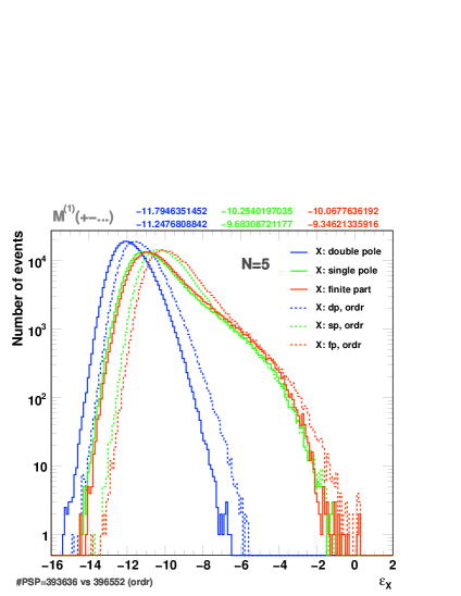
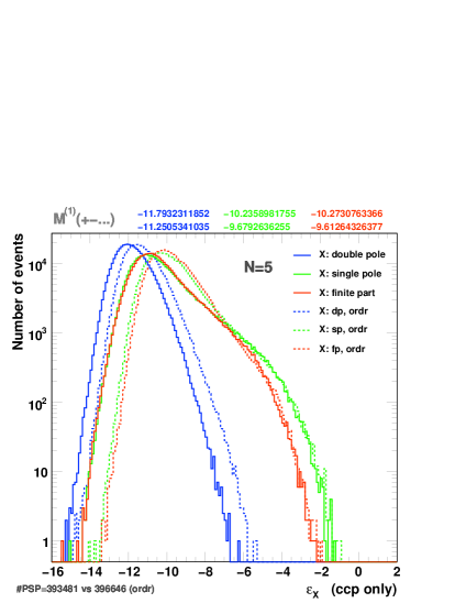
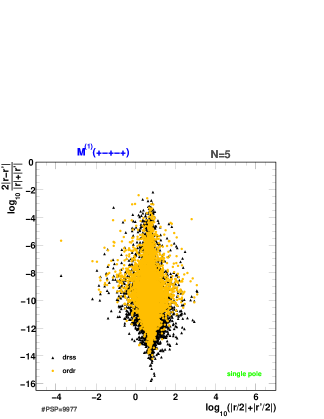
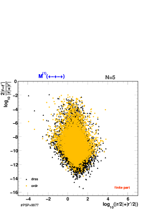
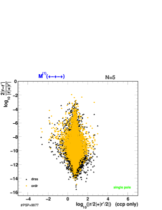
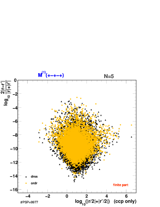
Figure 10: Double-, single-pole and finite-part accuracy distributions (upper part) and scatter graphs (lower part) extracted from double-precision computations of one-loop amplitudes for $n={\tt N}=5$ gluons with polarizations $\lambda_{k}=+-+-+$ and randomly chosen non-zero color configurations. The virtual corrections were calculated at random phase-space points satisfying the cuts detailed in the text. Unstable solutions were vetoed. Results from the color-dressed algorithm are compared with those of the color-ordered method indicated by dashed curves and brighter dots in the plots. The 5(4)-dimensional case is shown in the top left (right) and center (bottom) part of the figure. The definitions of $\varepsilon$ and $r$ are given in the text. All scatter graphs contain $2\times 10^{4}$ points.

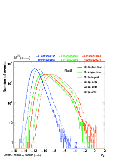
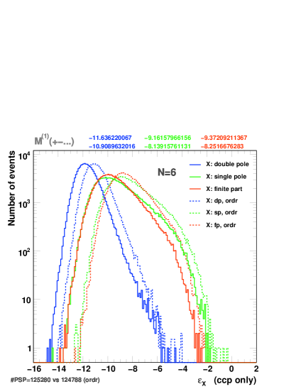
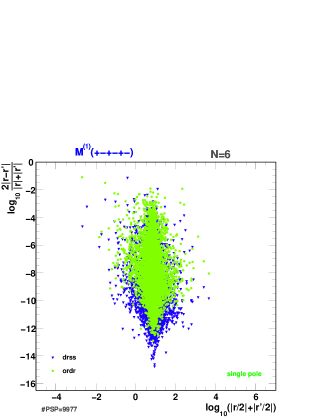
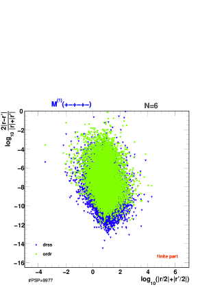
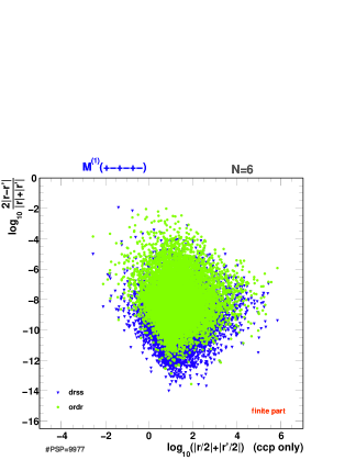
Figure 11: Double-, single-pole and finite-part accuracy distributions (upper part) and scatter graphs (lower part) extracted from double-precision computations of one-loop amplitudes for $n={\tt N}=6$ gluons with polarizations $\lambda_{k}=+-+-+-$ and randomly chosen non-zero color configurations. The virtual corrections were calculated at random phase-space points satisfying the cuts detailed in the text. Unstable solutions were vetoed. Results from the color-dressed algorithm are compared with those of the color-ordered method indicated by dashed curves and brighter dots in the plots. The 5(4)-dimensional case is shown in the top left (right) and center (bottom) part of the figure. The definitions of $\varepsilon$ and $r$ are given in the text. All scatter graphs contain $2\times 10^{4}$ points.

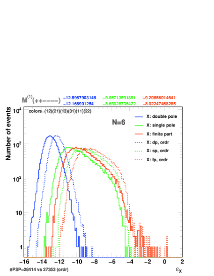
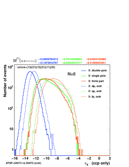
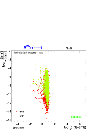
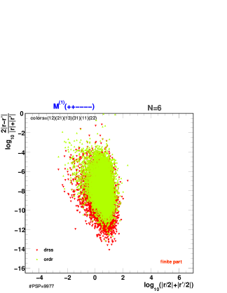
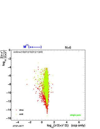
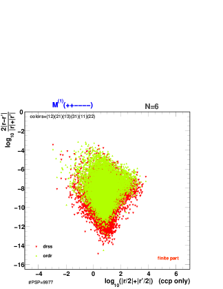
Figure 12: Double-, single-pole and finite-part accuracy distributions (upper part) and scatter graphs (lower part) as obtained from double-precision evaluations of one-loop amplitudes for $n={\tt N}=6$ gluons with polarizations and colors set to $\lambda_{k}=++----$ and $(ij)_{k}=(12)(21)(13)(31)(11)(22)$, respectively. The virtual corrections were calculated at random phase-space points satisfying the cuts detailed in the text. The veto procedure has been applied to reject unstable solutions. The results given by the color-dressed algorithm are compared with those of the color-ordered method indicated by dashed curves and brighter dots in the plots. The 5(4)-dimensional case is shown in the top left (right) and center (bottom) part of the figure. The definitions of $\varepsilon$ and $r$ are given in the text. Each scatter graph contains $2\times 10^{4}$ points. $94.7$($94.1$)% and $91.2$($91.0$)% of the events pass all tests in the dressed and ordered “5(4)D-case”, respectively.

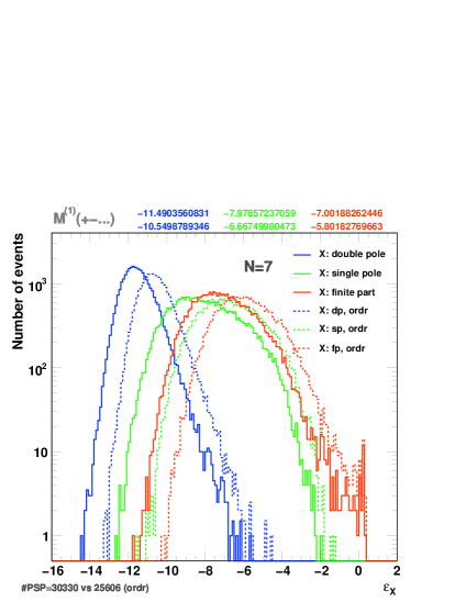
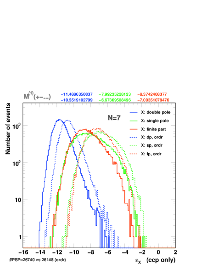
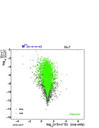
Figure 13: Double-, single-pole and finite-part accuracy distributions (upper part) and scatter graphs (lower part) extracted from double-precision computations of one-loop amplitudes for $n={\tt N}=7$ gluons with polarizations $\lambda_{k}=+-+-+-+$ and randomly chosen non-zero color configurations. The virtual corrections were calculated at random phase-space points satisfying the cuts detailed in the text. Unstable solutions were vetoed. Results from the color-dressed algorithm are compared with those of the color-ordered method indicated by dashed curves and brighter dots in the plots. The 5(4)-dimensional case is shown in the top left (right) and center (bottom) part of the figure. The definitions of $\varepsilon$ and $r$ are given in the text. All scatter graphs contain $2\times 10^{4}$ points.

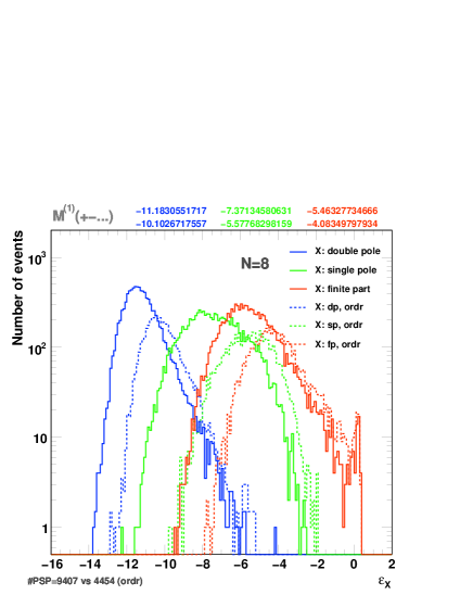
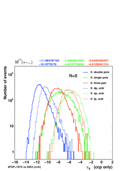
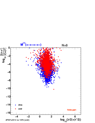
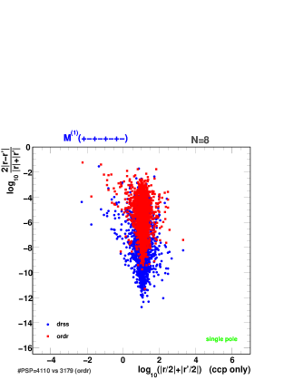
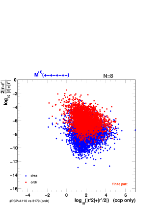
Figure 14: Double-, single-pole and finite-part accuracy distributions (upper part) and scatter graphs (lower part) extracted from double-precision computations of one-loop amplitudes for $n={\tt N}=8$ gluons with polarizations $\lambda_{k}=+-+-+-+-$ and randomly chosen non-zero color configurations. The virtual corrections were calculated at random phase-space points satisfying the cuts detailed in the text. Unstable solutions were vetoed. Results from the color-dressed algorithm are compared with those of the color-ordered method indicated by dashed curves and brighter dots in the plots. The 5(4)-dimensional case is shown in the top left (right) and center (bottom) part of the figure. The definitions of $\varepsilon$ and $r$ are given in the text; the number of points contained by each scatter graph is found in the lower left.

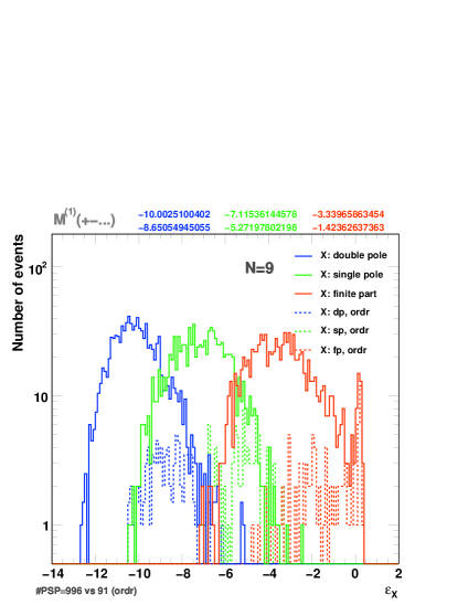
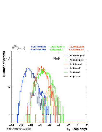
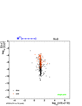
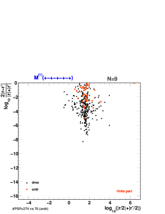
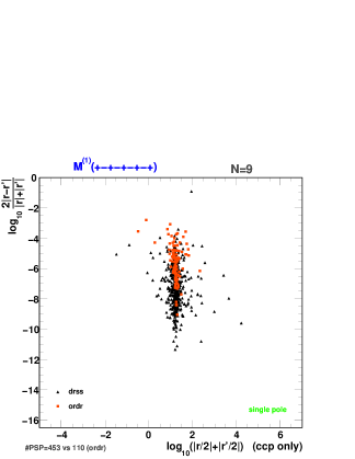
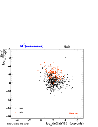
Figure 15: Double-, single-pole and finite-part accuracy distributions (upper part) and scatter graphs (lower part) extracted from double-precision computations of one-loop amplitudes for $n={\tt N}=9$ gluons with polarizations $\lambda_{k}=+-+-+-+-+$ and randomly chosen non-zero color configurations. The virtual corrections were calculated at random phase-space points satisfying the cuts detailed in the text. Unstable solutions were vetoed. Results from the color-dressed algorithm are compared with those of the color-ordered method indicated by dashed curves and brighter dots in the plots. The 5(4)-dimensional case is shown in the top left (right) and center (bottom) part of the figure. The definitions of $\varepsilon$ and $r$ are given in the text; the number of points contained by each scatter graph is found in the lower left.

In the upper part of Figs. 9-15 we show the distributions of relative accuracies $\varepsilon$ as occurring in the evaluation of gluon loop corrections with $n=4,\ldots,9$ external gluons. The lower part of these figures and Figs. 16 and 17 themselves depict scatter graphs visualizing the relative accuracies as a function of the size of the virtual corrections for the single pole and finite contributions only, as the double pole contribution has no observable variance. This form of presenting the results has information on whether certain points dominate the uncertainty of the total correction when averaging over the phase space. The $r$-variables used in these plots are defined by

$$r\;=\;\frac{1}{2\,\pi}\;\frac{\Re\left({{\cal M}^{(0)}}^{\dagger}{\cal M}^{(1)}\right)}{\left|\,{\cal M}^{(0)}\right|^{2}}$$ (67)

and represent corrections of the order of $\alpha_{s}$. Specifically, the $r$, $r^{\prime}$ and $r_{\rm th}$ given in the plots are obtained by employing ${\cal M}^{(1)}={\cal M}^{(1)[1]}_{\rm d/s/fp,num}$, ${\cal M}^{(1)}={\cal M}^{(1)[2]}_{\rm s/fp,num}$ and ${\cal M}^{(1)}={\cal M}^{(1)}_{\rm dp,th}$, respectively. In all cases we have rejected events with unreliable basis vectors in orthogonal space. Except for the results presented in Fig. 17, we have vetoed all events that led to unstable solutions of the bubble master-integral coefficient using $\Delta_{\rm veto}=0.02$. The statistics concerning these rejections is shown in Table 10.

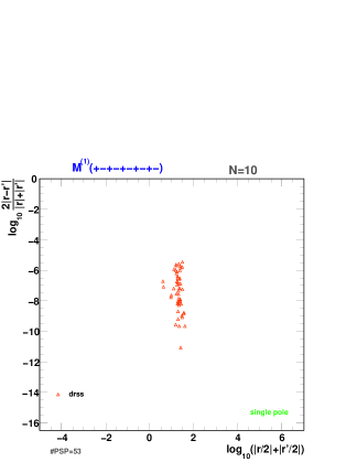
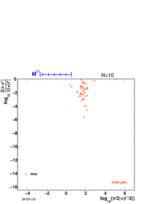
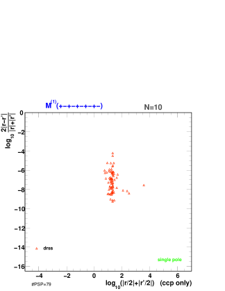
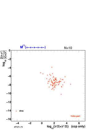
Figure 16: Single-pole and finite-part scatter graphs extracted from the double-precision computation of one-loop amplitudes for $n={\tt N}=10$ gluons with polarizations $\lambda_{k}=+-+-+-+-+-$ and randomly chosen non-zero color configurations. The virtual corrections were calculated at random phase-space points satisfying the cuts as described in the text. Unstable solutions were vetoed and, therefore, not included in the plots. The upper (lower) row of plots shows the results obtained from the 5(4)-dimensional color-dressed algorithm. For the definition of $r$, see text. The number of points contained by each scatter graph can be found in the lower left.

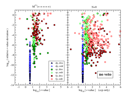
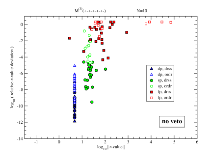
Figure 17: Double-, single-pole and finite-part scatter graphs visualizing the accuracy of double-precision evaluations of one-loop amplitudes for $n={\tt N}=9$ and $10$ gluons of alternating polarizations. Non-zero randomly chosen color configurations were used. Note that unstable solutions were not vetoed and therefore included in this presentation. The virtual corrections were calculated at random phase-space points satisfying the cuts as described in the text. Results of the 5-dimensional algorithms either based on color ordering (ordr) or color dressing (drss) are shown; for $n={\tt N}=9$, the “4D-case” results are also given (ccp only). For the definition of $r$, see text; axis labels as used in Fig. 16 are understood. The rightmost graph contains ${\cal O}(20)$ points per $\epsilon$-pole, while the left plot of the “5(4)D-case” has approximately $50$($120$) points per pole.

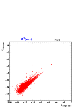
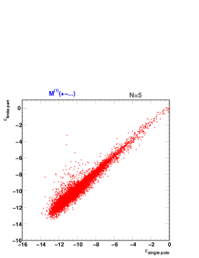
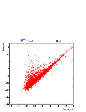
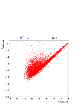
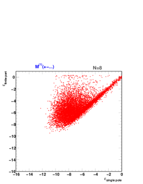
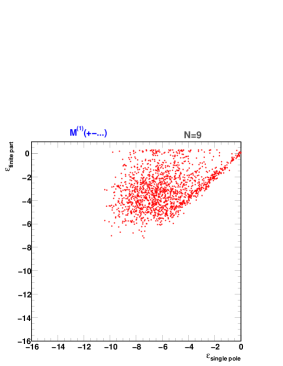
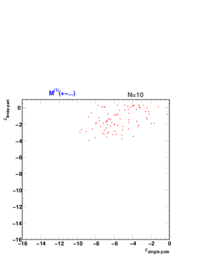
Figure 18: Finite-part versus single-pole accuracy (in double precision) as achieved in one-loop amplitude calculations using the color-dressed approach for various numbers $n={\tt N}$ of external gluons with polarizations $\lambda_{k}=+-\ldots+-(+)$ and colors randomly chosen among non-zero configurations. Note that unstable solutions have not been vetoed. The $n={\tt N}=9$ and $n={\tt N}=10$ graphs only contain $1.6\cdot 10^{3}$ and $87$ points, respectively, whereas all other plots comprise $10^{4}$ points.

We compare in all plots of Figs. 9-15 the color-dressed with the color-ordered approach where the results of the latter are indicated by dashed curves in the spectra (with the $\langle\varepsilon\rangle$ given by the lower top row of numbers) and brighter points in the scatter graphs. The $\varepsilon$ spectra of the “5D-case” (“4D-case”) are always shown in the top left (right) parts of the figures; the associated scatter graphs are compiled in the center (bottom) parts. In Fig. 16 we present our results for $n=10$ gluons where for reasons of limited statistics we solely show the scatter graphs related to the dressed method. The veto procedure has a very strong impact on ${\cal M}_{9,10}^{(1)}$ calculations. For the purpose of direct comparisons between vetoed and non-vetoed samples, we have added in Fig. 17 scatter plots that include vetoed events.

In all cases we notice that the double poles are obtained very accurately with almost no loss in precision for increasing number of gluons. The $n$-dependence of the single-pole and finite-part precisions is not as stable as for the double pole. We see noticeable shifts of the peak and mean positions towards larger values when incrementing the number of external gluons. The distribution’s tails are under good control. Because of the introduced veto procedure, they quickly die off around $\varepsilon\approx-2$. In rare cases worse accuracies occur, which happens more frequently for the 5-dimensional calculations. We can avoid these cases, if we extend the veto criteria by re-solving for and testing the rational bubble coefficient as well. For $n>9$, the limitations of double-precision computations unavoidably lead to rather unreliable single-pole and finite-part determinations. As an interesting fact, we observe that the color-dressed method yields throughout results of higher precision. Moreover, the decrease in accuracy for growing $n$ is more moderate compared to the method based on color ordering. Clearly, on the one hand this algorithm has to be run for many orderings and may therefore lead to an accumulation of small imprecisions. On the other hand a rather inaccurate determination of $m^{(1)}$ may appear just for a single ordering, in turn spoiling the overall result. Both effects make the ordered approach less capable of delivering accurate results. Turning to the scatter plots, we find that the most accurate but also inaccurate evaluations occur for points distributed near the vertical line of ${\cal O}(1)$ corrections. It is very encouraging that all top right quadrants are rather sparsely populated, dispelling the doubts that insufficiently determined large corrections may dominate our final results. The scatter regions of the double-pole solutions remain almost unchanged for larger $n$, while those of the single poles and finite parts are slightly growing gradually shifting towards lower relative accuracies. The scatter patches of the dressed method are displaced with respect to those of the color-decomposition approach: advantageously, they cover regions of greater precision, in particular populate the bottom right quadrants more densely. Due to the simplicity of the 4-gluon kinematics, the case of $n=4$ gluons stands out from the rest: the single pole and finite part can be obtained with almost the same accuracy as the double pole. This feature is preserved even if rational-part calculations are included. With $5$ gluons or more it is common that all coefficients contribute to the decomposition of the one-loop amplitude. The relative accuracies of the single poles and finite parts therefore develop a much different, less steeper, tail compared to the double poles. There are almost no differences between the double- and single-pole results obtained from the 4- and 5-dimensional algorithms. This is no surprise, since the coefficients necessary to reconstruct these poles can be determined in $4$ dimensions and our algorithms have been set up accordingly. In the absence of rational-part calculations it turns out that the finite parts may on average be obtained slightly more precisely than the single poles. The tails of the $1/\epsilon$ spectra reach out to the largest $\varepsilon$-values occurring in the evaluation of the cut-constructible part. The behavior is reversed in the 5-dimensional case owing to the addition of the rational part. For the same reason, we note increased $\langle\varepsilon_{\rm fp}\rangle$ in the “5D-case”, furthermore, the 5-dimensional scatter graphs show higher densities with respect to the 4-dimensional ones at lower accuracies.

As a special case of Fig. 11 we have displayed in Fig. 12 accuracy distributions and scatter plots for $n=6$ gluons of polarizations $\lambda_{k}=++----$ when instead of random color-space points the fixed non-zero color configuration $(ij)_{k}=(12)(21)(13)(31)(11)(22)$ has been selected. We notice that all $\varepsilon$-spectra are shifted towards smaller accuracies. Also, as illustrated by the scatter graphs, the magnitude of the virtual corrections is bound at ${\cal O}(1)$ with the exception of the finite piece of the cut-constructible part of the one-loop amplitudes. Interestingly, this is corrected back by adding in the rational part.

In Ref. [30] it was shown that the finite-part accuracy of the evaluation of ordered amplitudes is mostly correlated with that of the single poles. We have studied this issue for the dressed algorithm in the “5D-case”. The corresponding scatter plots also include the vetoed events and are presented in Fig. 18. The multitude of points is distributed along the diagonal indicating a strong correlation. As for color-ordered amplitudes the evaluation of the rational part becomes more involved with increasing gluon numbers. Therefore, regions of lower finite-part precision start to get populated distorting the diagonal trend.

Finally, we want to show that the Monte Carlo sampling as defined in Eq. (44) converges sufficiently fast for the color-dressed calculated virtual corrections. To this end we generalize the LO discussion following Eq. (35) with the details given in Sec. 3.3. The relevant quantity to explore in the Monte Carlo averaging is

$$S^{(0+1)}_{\rm MC}\;=\;\frac{1}{N_{\rm colpts}}\sum_{k=1}^{N_{\rm colpts}}W_{\rm col}(n_{1},n_{2},n_{3})\times\left[\,\left|\,{\cal M}^{(0)}_{k}\right|^{2}+\,\frac{\widehat{\alpha}_{s}}{2\,\pi}\,\Re\left({\cal M}_{{\rm fp},k}^{(1)}\,{{\cal M}_{k}^{(0)}}^{\dagger}\right)\,\right]$$ (68)

where we choose $\widehat{\alpha}_{S}=0.12$ and ${\cal M}_{{\rm fp},k}^{(1)}$ is the finite part of the virtual corrections. The sum over the $N_{\rm colpts}$ color configurations for each phase-space point is an optional “mini-Monte Carlo” over colors for faster convergence as a function of the number of phase-space point evaluations. By adding the real corrections to Eq. (68) and performing the coupling constant renormalization and mass factorization, one obtains the gluonic contribution to the NLO multi-jet differential cross section. Therefore, the convergence of Eq. (68) is the relevant quantity to study.

\psfrag{Yconvergelabel}[b][c][0.84]{ $\left(\left\langle S^{(0+1)}_{\rm MC}\right\rangle\pm\sigma_{\left\langle S^{(0+1)}_{\rm MC}\right\rangle}\right)\;\left\langle\,S^{(0+1)}_{\rm col}\right\rangle^{-1}$}\psfrag{Xconvergelabel}[b][b][0.44]{$100\%\times\sigma\Big{(}R^{(0+1)}_{\rm MC}(N_{\rm MC})\Big{)}\Big{/}\mu\Big{(}R^{(0+1)}_{\rm MC}(N_{\rm MC})\Big{)}$}\includegraphics[width=277.51653pt,angle={-90}]{plots/4/I4LL.p.ps}

Figure 19: Consistency test for the Monte Carlo integration of 4-gluon virtual corrections using “Non-Zero” color sampling compared to the exact color summing. As a function of the number $N_{\rm MC}$ of evaluated phase-space points the $R^{(0+1)}$-ratio is plotted converging to one as it should be. The inserted plot shows the number of phase-space evaluations needed to reach a given relative accuracy in terms of $R^{(0+1)}_{\rm MC}(N_{\rm MC})$ while Monte Carlo integrating; for the definitions, see text. The dashed line depicts the fit function $\sigma/\mu=A\,N_{\rm MC}^{-B}$, see also Table 11.

By defining the $n$-gluon color-summed counterpart of $S^{(0+1)}_{\rm MC}$,

$$S_{\rm col}^{(0+1)}\;=\sum_{i_{1},\ldots,i_{n}=1}^{3}\ \sum_{j_{1},\ldots,j_{n}=1}^{3}\left[\,\left|\,{\cal M}_{k}^{(0)}\right|^{2}+\,\frac{\widehat{\alpha}_{s}}{2\,\pi}\,\Re\left({\cal M}_{{\rm fp},k}^{(1)}\,{{\cal M}_{k}^{(0)}}^{\dagger}\right)\,\right]\ ,$$ (69)

we can form the ratios

$$R^{(0+1)}\;=\;\frac{\langle S^{(0+1)}_{\rm MC}\rangle\,\pm\,\sigma_{\langle S^{(0+1)}_{\rm MC}\rangle}}{\langle S^{(0+1)}_{\rm col}\rangle}\ ,\qquad R^{({\rm V})}\;=\;\frac{\langle S^{(0+1)}_{\rm MC}\rangle\,\pm\,\sigma_{\langle S^{(0+1)}_{\rm MC}\rangle}}{\langle S^{(0)}_{\rm col}\rangle}$$ (70)

analogously to Eq. (37). We define the mean values and standard deviations of the ratios similarly to Eqs. (38) and (39), respectively. Note that $S^{(0)}_{\rm col}$ is already defined at LO by Eq. (36). As we increase the number of Monte Carlo points, $N_{\rm MC}$, the $R^{({\rm V})}$-ratios quantify the relative importance of the virtual corrections, while the $R^{(0+1)}$-ratios should converge to one. For the latter, this is nicely demonstrated in Fig. 19 for the 4-gluon virtual corrections and the “Non-zero” sampling scheme as described in Sec. 3.3. After $15900$ events we obtain $R^{(0+1)}=0.939\pm 0.039$, which is satisfactory for this consistency check.

As in the LO discussion we want to illustrate how many events are needed to achieve a certain relative integration uncertainty when performing the Monte Carlo color sampling. In analogy to Eq. (40) we can construct the ratio

$$R^{(0+1)}_{\rm MC}(N_{\rm MC})\;=\;\frac{\sum_{r=1}^{N_{\rm MC}}S^{(0+1)}_{{\rm MC},r}}{\sum_{r=1}^{N_{\rm MC}}S^{(0+1)}_{{\rm col},r}}$$ (71)

as a function of $N_{\rm MC}$. Again, it is interesting to change the normalization of the ratio and also define

$$R^{({\rm V})}_{\rm MC}(N_{\rm MC})\;=\;\frac{\sum_{r=1}^{N_{\rm MC}}S^{(0+1)}_{{\rm MC},r}}{\sum_{r=1}^{N_{\rm MC}}S^{(0)}_{{\rm col},r}}$$ (72)

in order to study the impact of the virtual corrections. As before we partition $N_{\rm event}=N_{\rm trial}\times N_{\rm MC}$ events to have a certain number of trials to compute the corresponding mean values $\mu$ and standard deviations $\sigma$ for $n$-gluon LO and virtual scattering according to Eqs. (41) and (42), respectively. For the case of $R^{(0+1)}_{\rm MC}(N_{\rm MC})$ and 4-gluon scattering, the number of Monte Carlo points versus a given relative accuracy is shown in the inlaid plot of Fig. 19. As at LO, the curve bends behaving as statistically determined after a certain amount of Monte Carlo integration steps.

:)	Naive		Conserved				Non-Zero				Non-Zero, $N_{\rm colpts}=4$
$n$	$B$	$A$	$B$	$A$	$A^{\prime}$	$f$	$B$	$A$	$A^{\prime}$	$f$	$B$	$A$	$A^{\prime}$	$f$
4∗							0.479	3.36
4	0.497	22.0	0.489	5.41	17.0	10.4	0.476	3.57	13.5	16.4	0.485	2.05	15.6	65.7
5	0.482	59.4	0.454	13.3	43.3	13.5	0.442	9.71	36.4	19.8	0.439	5.56	37.8	79.2
6	0.325	7.08	0.344	5.37	14.0	16.3	0.255	1.60	3.50	21.7	0.233	0.850	2.14	87.6

Table 11: Parameter values $B$, $A$ and $A^{\prime}$ obtained from curve fitting of the $\sigma(R_{\rm MC})/\mu(R_{\rm MC})$ to the functional form $A\times N_{\rm MC}^{-B}$. The results are given for the different ways of sampling over colors in $n$-gluon scattering. The 4-gluon case marked by “$\ast$” corresponds to the consistency check shown in Fig. 19, where $R^{(0+1)}_{\rm MC}$ has been considered. In all other cases $R^{({\rm V})}_{\rm MC}$ has been used, cf. Figs. 20, 21 and 22. Note that for $n=6$, we have fitted $\sigma(R^{({\rm V})}_{\rm MC})$. The parameters $A^{\prime}=Af^{B}$ take into account that the evaluation of a fixed number of Monte Carlo events takes longer for the other than “Naive” color-sampling methods. The time factors $f$ relative to the “Naive” case are also displayed.

To quantify the color-integration performances, we again perform fits to the functional form $A\times N_{\rm MC}^{-B}$ and show the values of the fitted parameters in Table 11 for the various cases. As argued in Sec. 3.3 for large enough $N_{\rm MC}$, we expect a scaling of $\sigma/\mu$ that is proportional to $1/\sqrt{N_{\rm MC}}$. The goodness of the sampling schemes is signified by the $A$- and $A^{\prime}$-parameters, where the latter is more important since the time factors are included. Smaller values of these parameters indicate a better efficiency of the sampling procedure.

:)	Naive		Conserved		Non-Zero		Non-Zero, $N_{\rm colpts}=4$
$n$	$N_{\rm MC}$	$R^{({\rm V})}$	$N_{\rm MC}$	$R^{({\rm V})}$	$N_{\rm MC}$	$R^{({\rm V})}$	$N_{\rm MC}$	$R^{({\rm V})}$
4	$4\cdot\!10^{6}$	$0.4739\pm 0.0054$	$4\cdot\!10^{6}$	$0.4750\pm 0.0017$	$4\cdot\!10^{6}$	$0.4724\pm 0.0013$	$1\cdot\!10^{6}$	$0.4738\pm 0.0020$
5	631K	$0.241\pm 0.022$	631K	$0.2673\pm 0.0072$	631K	$0.2744\pm 0.0058$	160K	$0.2790\pm 0.0058$
6	64K	$-0.10\pm 0.12$	64K	$-0.059\pm 0.094$	50.2K	$-0.076\pm 0.062$	16K	$-0.044\pm 0.066$
7	4K	$-0.87\pm 0.66$	4K	$-0.23\pm 0.09$	4K	$-0.14\pm 0.10$	2K	$-0.97\pm 0.65$

Table 12: Monte Carlo integration results for the $R^{({\rm V})}$ ratios as defined in the text after $N_{\rm MC}$ phase-space point evaluations for $n$-gluon scattering and different color-sampling schemes using color-dressed tree-level and one-loop amplitude calculations.

Using the $R^{({\rm V})}$ and $R^{({\rm V})}_{\rm MC}(N_{\rm MC})$ ratios, we summarize in Figs. 20-23 our Monte Carlo integration results for $n=4,\ldots,7$ gluon processes and for the various color-sampling schemes. The upper graphs display the averaging of $S_{\rm MC}^{(0+1)}$ normalized to the Monte Carlo average of the color-summed LO contribution as a function of the number of phase-space evaluations. We also indicate the estimate of the integration uncertainty, see Eqs. (70) and (39). To compare all different test cases, Table 12 list the final values for $R^{({\rm V})}$. In all these figures we plot in the lower graphs the number of phase-space point evaluations needed to reach a certain relative integration uncertainty on $R^{({\rm V})}_{\rm MC}(N_{\rm MC})$. We show in Table 11 the results of the curve fittings represented by the dashed lines in these plots.

As is clear from these Monte Carlo averaging tests and results, the convergence is more than satisfactory for future applications of the color-dressing techniques in NLO calculations. If faster sampling convergence is required we can evaluate multiple color configurations per phase-space point. This is shown in the graph, where we have chosen to evaluate four color configurations at one phase-space point.

\psfrag{Yconvergelabel}[b][c][0.84]{ $\left(\left\langle S^{(0+1)}_{\rm MC}\right\rangle\pm\sigma_{\left\langle S^{(0+1)}_{\rm MC}\right\rangle}\right)\;\left\langle\,\sum\limits_{\rm col}\left|{\cal M}^{(0)}\right|^{2}\right\rangle^{-1}$}\psfrag{Xconvergelabel}[t][t][0.84]{$100\%\times\sigma\Big{(}R^{({\rm V})}_{\rm MC}(N_{\rm MC})\Big{)}\Big{/}\mu\Big{(}R^{({\rm V})}_{\rm MC}(N_{\rm MC})\Big{)}$}\includegraphics[width=277.51653pt,angle={-90}]{plots/4/I4.p.ps}

\psfrag{Yconvergelabel}[b][c][0.84]{ $\left(\left\langle S^{(0+1)}_{\rm MC}\right\rangle\pm\sigma_{\left\langle S^{(0+1)}_{\rm MC}\right\rangle}\right)\;\left\langle\,\sum\limits_{\rm col}\left|{\cal M}^{(0)}\right|^{2}\right\rangle^{-1}$}\psfrag{Xconvergelabel}[t][t][0.84]{$100\%\times\sigma\Big{(}R^{({\rm V})}_{\rm MC}(N_{\rm MC})\Big{)}\Big{/}\mu\Big{(}R^{({\rm V})}_{\rm MC}(N_{\rm MC})\Big{)}$}\includegraphics[width=277.51653pt,angle={-90}]{plots/4/I4Nmc.p.ps}

Figure 20: Upper graph: convergence of the 4-gluon virtual corrections integration as a function of the number of evaluated phase-space points. Also shown is the standard deviation as an estimator of the integration uncertainty. Lower graph: convergence of the Monte Carlo integration, where the relative integration uncertainty is shown as a function of the number of phase-space evaluations. The dashed lines describe the fit functions $\sigma/\mu=A\,N_{\rm MC}^{-B}$, see also Table 11. The “Naive”, “Conserved” and “Non-Zero” color-sampling methods are explained in Sec. 3.3. The points indicated by “Non-Zero, $N_{\rm colpts=4}$” average over 4 color configurations per phase-space point.

\psfrag{Yconvergelabel}[b][c][0.84]{ $\left(\left\langle S^{(0+1)}_{\rm MC}\right\rangle\pm\sigma_{\left\langle S^{(0+1)}_{\rm MC}\right\rangle}\right)\;\left\langle\,\sum\limits_{\rm col}\left|{\cal M}^{(0)}\right|^{2}\right\rangle^{-1}$}\psfrag{Xconvergelabel}[t][t][0.84]{$100\%\times\sigma\Big{(}R^{({\rm V})}_{\rm MC}(N_{\rm MC})\Big{)}\Big{/}\mu\Big{(}R^{({\rm V})}_{\rm MC}(N_{\rm MC})\Big{)}$}\includegraphics[width=277.51653pt,angle={-90}]{plots/5/I5.p.ps}

\psfrag{Yconvergelabel}[b][c][0.84]{ $\left(\left\langle S^{(0+1)}_{\rm MC}\right\rangle\pm\sigma_{\left\langle S^{(0+1)}_{\rm MC}\right\rangle}\right)\;\left\langle\,\sum\limits_{\rm col}\left|{\cal M}^{(0)}\right|^{2}\right\rangle^{-1}$}\psfrag{Xconvergelabel}[t][t][0.84]{$100\%\times\sigma\Big{(}R^{({\rm V})}_{\rm MC}(N_{\rm MC})\Big{)}\Big{/}\mu\Big{(}R^{({\rm V})}_{\rm MC}(N_{\rm MC})\Big{)}$}\includegraphics[width=277.51653pt,angle={-90}]{plots/5/I5Nmc.p.ps}

Figure 21: Upper graph: convergence of the 5-gluon virtual corrections integration as a function of the number of evaluated phase-space points. Also shown is the standard deviation as an estimator of the integration uncertainty. Lower graph: convergence of the Monte Carlo integration, where the relative integration uncertainty is shown as a function of the number of phase-space evaluations. The dashed lines describe the fit functions $\sigma/\mu=A\,N_{\rm MC}^{-B}$, see also Table 11. The “Naive”, “Conserved” and “Non-Zero” color-sampling methods are explained in Sec. 3.3. The points indicated by “Non-Zero, $N_{\rm colpts=4}$” average over 4 color configurations per phase-space point.

\psfrag{Yconvergelabel}[b][c][0.84]{ $\left(\left\langle S^{(0+1)}_{\rm MC}\right\rangle\pm\sigma_{\left\langle S^{(0+1)}_{\rm MC}\right\rangle}\right)\;\left\langle\,\sum\limits_{\rm col}\left|{\cal M}^{(0)}\right|^{2}\right\rangle^{-1}$}\psfrag{XXconvergelabel}[t][t][0.84]{$\sigma\Big{(}R^{({\rm V})}_{\rm MC}(N_{\rm MC})\Big{)}$}\includegraphics[width=277.51653pt,angle={-90}]{plots/6/I6.p.ps}

\psfrag{Yconvergelabel}[b][c][0.84]{ $\left(\left\langle S^{(0+1)}_{\rm MC}\right\rangle\pm\sigma_{\left\langle S^{(0+1)}_{\rm MC}\right\rangle}\right)\;\left\langle\,\sum\limits_{\rm col}\left|{\cal M}^{(0)}\right|^{2}\right\rangle^{-1}$}\psfrag{XXconvergelabel}[t][t][0.84]{$\sigma\Big{(}R^{({\rm V})}_{\rm MC}(N_{\rm MC})\Big{)}$}\includegraphics[width=277.51653pt,angle={-90}]{plots/6/I6Nmc.p.ps}

Figure 22: Upper graph: convergence of the 6-gluon virtual corrections integration as a function of the number of evaluated phase-space points. Also shown is the standard deviation as an estimator of the integration uncertainty. Lower graph: convergence of the Monte Carlo integration, where this time the standard deviation is shown as a function of the number of phase-space evaluations. Note that for this case, the virtual corrections are as large as the LO contribution so that the full result is close to zero. The dashed lines describe the fit functions $\sigma=A\,N_{\rm MC}^{-B}$, see also Table 11. The “Naive”, “Conserved” and “Non-Zero” color-sampling methods are explained in Sec. 3.3. The points indicated by “Non-Zero, $N_{\rm colpts=4}$” average over 4 color configurations per phase-space point.

\psfrag{Yconvergelabel}[b][c][0.84]{ $\left(\left\langle S^{(0+1)}_{\rm MC}\right\rangle\pm\sigma_{\left\langle S^{(0+1)}_{\rm MC}\right\rangle}\right)\;\left\langle\,\sum\limits_{\rm col}\left|{\cal M}^{(0)}\right|^{2}\right\rangle^{-1}$}\psfrag{XXconvergelabel}[t][t][0.84]{$\sigma\Big{(}R^{({\rm V})}_{\rm MC}(N_{\rm MC})\Big{)}$}\includegraphics[width=277.51653pt,angle={-90}]{plots/7/I7.p.ps}

\psfrag{Yconvergelabel}[b][c][0.84]{ $\left(\left\langle S^{(0+1)}_{\rm MC}\right\rangle\pm\sigma_{\left\langle S^{(0+1)}_{\rm MC}\right\rangle}\right)\;\left\langle\,\sum\limits_{\rm col}\left|{\cal M}^{(0)}\right|^{2}\right\rangle^{-1}$}\psfrag{XXconvergelabel}[t][t][0.84]{$\sigma\Big{(}R^{({\rm V})}_{\rm MC}(N_{\rm MC})\Big{)}$}\includegraphics[width=277.51653pt,angle={-90}]{plots/7/I7Nmc.p.ps}

Figure 23: Upper graph: convergence of the 7-gluon virtual corrections integration as a function of the number of evaluated phase-space points. Also shown is the standard deviation as an estimator of the integration uncertainty. Lower graph: convergence of the Monte Carlo integration, where for this case, only the standard deviation is shown as a function of the number of phase-space evaluations. The “Naive”, “Conserved” and “Non-Zero” color-sampling methods are explained in Sec. 3.3. The points indicated by “Non-Zero, $N_{\rm colpts=4}$” average over 4 color configurations per phase-space point.

5 Conclusions

In this paper we explored the possibility of color sampling within the context of $D$-dimensional generalized unitarity. Up to now generalized unitarity has only been used within the context of color-ordered primitive amplitudes. In the color-ordered approach, color is treated differently from the other quantum numbers such as spin and flavor. This makes the reconstruction of the full one-loop amplitude rather cumbersome.

We have reformulated the $D$-dimensional generalized unitarity formalism to include color dressing. That is, we choose the explicit color of each parton, together with all other quantum numbers, for each Monte Carlo event. In this way all particles, colored or colorless, are treated on an equal footing. There is no distinction between different particles as far as the formalism goes. Consequently, the resulting algorithm is independent of the type and flavor of the external particles. E.g. the same algorithm calculates the 6-gluon virtual corrections, the 6-photon virtual corrections and the $W$+6 parton virtual corrections.

The use of unordered amplitudes requires the partition of the external legs into unordered subsets. This is necessary for the calculation of the tree-level amplitudes as well as for generating all the unitarity cuts. As a result the complexity of the resulting algorithm is exponential. That is, the computer time needed to calculate the virtual corrections grows with a constant multiplicative factor when one adds external particles. In addition, we have to sum over all color states of the internal lines. One may conclude from these general features that the implementation of the color-dressed $D$-dimensional generalized unitarity is less efficient in comparison with an implementation based on ordered primitive amplitudes. As we have explicitly demonstrated for the example of calculating the virtual corrections to $n$-gluon scattering, this is not the case. We compared the color-sampling approach for both the color-ordered and color-dressed case. The calculation of the virtual corrections in the color-dressed case scales as $7^{n}$, while in the color-ordered case the effective scaling up to 10 gluons behaves as $9^{n}$. Moreover, the color-dressed calculation has a better accuracy in calculating the value of the one-loop amplitude. The improved accuracy over color-ordered evaluations increases with $n$.

As we showed for $n$-gluon scattering, the color-dressed approach becomes more efficient than the color-ordered method for large $n$. One could argue that the differences are small and color sampling over the ordered $n$-gluon amplitudes will work as well. However, when including quarks and other electro-weak particles the color-dressed approach will easily win out over the color-ordered approach. This is because any notion of primitive amplitudes is absent. The algorithm simply calculates the virtual correction. Moreover, the color-dressed algorithm remains identical when including quarks and electro-weak particles. It is this algorithmic simplicity that will enable us to employ parallel programming to significantly improve the computer evaluation time.

We conclude that the color-dressed formulation is competitive for calculating one-loop virtual corrections for $n$-gluon scattering. It is expected that it will be even more efficient in calculating virtual corrections for processes involving quarks and electro-weak gauge bosons in addition to the gluons.

Appendix A The Tree-Level 6-Quark Amplitude

As an example we can take a few recursive steps in calculating the 6-quark tree-level matrix element. We start with the definition of the tree-level matrix element in terms of the 5-quark fermionic current

$${\cal M}^{(0)}\left({\bf u},{\bf\bar{u}},{\bf d},{\bf\bar{d}},{\bf s},{\bf\bar{s}}\right)\;=\;P^{-1}\left[J\left({\bf u},{\bf\bar{u}},{\bf d},{\bf\bar{d}},{\bf s}\right),J\left({\bf\bar{s}}\right)\right]$$ (73)

where we use the shorthand notation ${\bf u}=u_{i_{1}}^{\lambda_{1}}(K_{1})$, ${\bf\bar{u}}=\bar{u}_{j_{1}}^{-\lambda_{1}}(K_{2})$, ${\bf d}=d_{i_{2}}^{\lambda_{2}}(K_{3})$, ${\bf\bar{d}}=\bar{d}_{j_{2}}^{-\lambda_{2}}(K_{4})$, ${\bf s}=s_{i_{3}}^{\lambda_{3}}(K_{5})$ and ${\bf\bar{s}}={\bar{s}}_{j_{3}}^{-\lambda_{3}}(K_{6})$. The 5-quark fermionic current decomposes into

$$J_{\bf\bar{s}}\left({\bf u},{\bf\bar{u}},{\bf d},{\bf\bar{d}},{\bf s}\right) = P_{\bf\bar{s}}\Big{[}D\big{[}J\left({\bf d},{\bf\bar{d}},{\bf s}\right),J\left({\bf u},{\bf\bar{u}}\right)\big{]}\Big{]}+P_{\bf\bar{s}}\Big{[}D\big{[}J\left({\bf u},{\bf\bar{u}},{\bf s}\right),J\left({\bf d},{\bf\bar{d}}\right)\big{]}\Big{]}$$ (74)

$$+ P_{\bf\bar{s}}\Big{[}D\big{[}J\left({\bf s}\right),J\left({\bf u},{\bf\bar{u}},{\bf d},{\bf\bar{d}}\right)\big{]}\Big{]}\ .$$

The 3-quark fermionic current decomposes into

$$J_{\bf\bar{s}}\left({\bf q},{\bf\bar{q}},{\bf s}\right)\;=\;P_{\bf\bar{s}}\Big{[}D\big{[}J\left({\bf s}\right),J\left({\bf q},{\bf\bar{q}}\right)\big{]}\Big{]}\ ,$$ (75)

where ${\bf q}\in\{{\bf u},{\bf d}\}$ and ${\bf\bar{q}}\in\{{\bf\bar{u}},{\bf\bar{d}}\}$. The 1-quark fermionic current is simply the source term. Finally the 4-quark gluonic current is given by

$$J_{\bf g}\left({\bf u},{\bf\bar{u}},{\bf d},{\bf\bar{d}}\right) = P_{\bf g}\Big{[}D\big{[}J\left({\bf u}\right),J\left({\bf d},{\bf\bar{d}},{\bf u}\right)\big{]}\Big{]}+P_{\bf g}\Big{[}D\big{[}J\left({\bf u},{\bf d},{\bf\bar{u}}\right),J\left({\bf\bar{u}}\right)\big{]}\Big{]}$$ (76)

$$+ P_{\bf g}\Big{[}D\big{[}J\left({\bf d}\right),J\left({\bf u},{\bf\bar{u}},{\bf d}\right)\big{]}\Big{]}+P_{g}\Big{[}D\big{[}J\left({\bf d},{\bf u},{\bf\bar{u}}\right),J\left({\bf\bar{d}}\right)\big{]}\Big{]}\ ,$$

and the 2-quark gluonic current is written as

$$J_{\bf g}\left({\bf q},{\bf\bar{q}}\right)\;=\;P_{\bf g}\Big{[}D\big{[}J\left({\bf q}\right),J\left({\bf\bar{q}}\right)\big{]}\Big{]}\ .$$ (77)

The above steps define the 6-quark LO amplitude recursively as would be done by the algorithm. Note that we have ignored all flavor violating currents.

Appendix B The Implemented Gluon Recursion Relation

Making use of the color-flow representation [32], we define the color-dressed gluon currents as $3\times 3$ matrices of ordered gluon currents:

$$J^{(IJ)}_{\mu}(g^{\lambda_{1}}_{1})\;=\;\delta^{I}_{j_{1}}\delta^{i_{1}}_{J}J_{\mu}(g^{\lambda_{1}}_{1})\ ,$$ (78)

where the external gluon $g_{1}$ has the polarization $\lambda_{1}$ and four-momentum $K_{1}$, its colors are denoted by $(ij)_{1}$. The color-flow labels of the dressed current are $(IJ)$ and $\mu$ indicates the Lorentz label. Using this definition, the connection to the compact notation introduced in Sec. 3.1 is found as

$$J_{\bf g}\big{(}{\bf g}_{1}\big{)}\;=\;\delta^{Ii_{1}}\delta^{Jj_{1}}\,\varepsilon_{\mu}^{\lambda_{1}}(K_{1})\;\equiv\;\delta^{J}_{j_{1}}\delta^{i_{1}}_{I}J_{\mu}(g^{\lambda_{1}}_{1})\;=\;J^{(JI)}_{\mu}(g^{\lambda_{1}}_{1})\ .$$ (79)

Since we only consider gluons, a plain numbering of the external particles ${\bf g}_{k}=\{g_{k},\lambda_{k},(ij)_{k},K_{k}\}$ is sufficient and helps simplify the notation such that the color dressing becomes more emphasized. Hence, in all what follows we write $J_{\bf g}({\bf 1})=\delta^{J}_{j_{1}}\delta^{i_{1}}_{I}J_{\mu}(1)=J^{(JI)}_{\mu}(1)$. Dressed $n$-gluon currents are then described by

$$J^{(IJ)}_{\mu}(1,2,\ldots,n)\;=\sum\limits_{\sigma\in S_{n}}\delta^{I}_{j_{\sigma_{1}}}\delta^{i_{\sigma_{1}}}_{j_{\sigma_{2}}}\cdots\delta^{i_{\sigma_{n-1}}}_{j_{\sigma_{n}}}\delta^{i_{\sigma_{n}}}_{J}\ J_{\mu}(\sigma_{1},\sigma_{2},\ldots,\sigma_{n})\ ,$$ (80)

which follows as a consequence of the color decomposition of the tree-level amplitude into ordered ones:

$${\cal M}^{(0)}(1,2,\ldots,n,n+1)\;=\sum\limits_{\sigma\in S_{n}}\delta^{i_{n+1}}_{j_{\sigma_{1}}}\delta^{i_{\sigma_{1}}}_{j_{\sigma_{2}}}\cdots\delta^{i_{\sigma_{n-1}}}_{j_{\sigma_{n}}}\delta^{i_{\sigma_{n}}}_{j_{n+1}}\ m^{(0)}(\sigma_{1},\sigma_{2},\ldots,\sigma_{n},n+1)\ .$$ (81)

The vectors $\sigma$ describe the elements of the permutations $S_{n}$ of the set $\{1,2,\ldots,n\}$. With the color-ordered amplitudes $m^{(0)}(\sigma_{1},\sigma_{2},\ldots,\sigma_{n},n+1)$ expressed through ordered $J$-currents and the definition of the dressed currents at hand, we can re-write the last equation and formulate the tree-level amplitude in terms of the color-dressed currents:

$${\cal M}^{(0)}(1,2,\ldots,n,n+1) = K^{2}_{\{1,2,\ldots,n\}}\;\times$$ (82)

$$\sum\limits_{\sigma\in S_{n}}\delta^{I}_{j_{\sigma_{1}}}\delta^{i_{\sigma_{1}}}_{j_{\sigma_{2}}}\cdots\delta^{i_{\sigma_{n-1}}}_{j_{\sigma_{n}}}\delta^{i_{\sigma_{n}}}_{J}\ J_{\mu}(\sigma_{1},\sigma_{2},\ldots,\sigma_{n})\ \delta^{J}_{j_{n+1}}\delta^{i_{n+1}}_{I}\ J^{\mu}(n+1)$$

$$= K^{2}_{\{1,2,\ldots,n\}}\ J^{(IJ)}_{\mu}(1,2,\ldots,n)\;J^{(JI),\;\!\mu}(n+1)\ .$$

Owing to the simple color structure of the one-gluon current, the summation over the color indices $(IJ)$ effectively reduces to the calculation of a single scalar product of the ordered currents $J^{(i_{n+1}\,j_{n+1})}_{\mu}$ and $J^{(j_{n+1}\,i_{n+1}),\;\!\mu}$. The invariant-mass prefactor $K^{2}$ is determined by the gluon momenta via $K^{2}_{\{1,2,\ldots,n\}}=(K_{1}+K_{2}+\ldots+K_{n})^{2}$. The one-gluon current is given in Eq. (78), while the multi-gluon current is obtained recursively. Starting from Eq. (80), one incorporates the ordered gluon recurrence relation to evaluate $J_{\mu}(\sigma_{1},\ldots,\sigma_{n})$ and re-groups accordingly to identify the partitioning. After some algebra, one finds

$$J^{IJ}_{\mu}(1,2,\ldots,n) = K^{-2}_{\{1,2,..,n\}}\,\Bigg{[}\;\ \sum_{P_{\pi_{1}\pi_{2}}(1,\ldots,n)}\Big{(}\delta^{ILN}_{KMJ}-\delta^{INL}_{MKJ}\Big{)}\left[J^{(KL)}_{\mu}(\pi_{1}),J^{(MN)}_{\mu}(\pi_{2})\right]\ +$$ (83)

$$\sum_{P_{\pi_{1}\pi_{2}\pi_{3}}(1,\ldots,n)}\Big{(}\delta^{ILNP}_{KMOJ}+\delta^{IPNL}_{OMKJ}-\delta^{ILPN}_{KOMJ}-\delta^{INPL}_{MOKJ}\Big{)}\ \times$$

$$\hskip 59.75078pt\bigg{(}\left\{J^{(KL)}_{\mu}(\pi_{1}),J^{(MN)}_{\mu}(\pi_{2}),J^{(OP)}_{\mu}(\pi_{3})\right\}\;+\;\pi_{1}\leftrightarrow\pi_{2}\bigg{)}\;\ \Bigg{]}$$

where we have employed the bracket notation for ordered-current operations, which was introduced in Ref. [20]. The partition sums are explained in Sec. 3.1 and an implicit summation over the color indices $K,L,M,N,O,P$ is understood. To efficiently compute the dressed currents, the color factors in front of the operator brackets can be pre-calculated such that the computation of zero color-weight contributions can be avoided. We have used the shorthand notation

$$\delta^{ik\cdots m}_{jl\cdots n}\;=\;\delta^{i}_{j}\delta^{k}_{l}\cdots\delta^{m}_{n}\ .$$ (84)

The recursion relation presented in Eq. (83) scales asymptotically as $4^{n}$, since we kept the 4-gluon vertex as an entity in our calculation. As a consequence we have to evaluate 3-subset partitions and the corresponding curly brackets that merge three different dressed currents.

References

- [1] T. Stelzer and W. F. Long, Comput. Phys. Commun. 81 (1994) 357 [arXiv:hep-ph/9401258].
- [2] M. L. Mangano, M. Moretti, F. Piccinini, R. Pittau and A. D. Polosa, JHEP 0307 (2003) 001 [arXiv:hep-ph/0206293].
- [3] P. D. Draggiotis, R. H. P. Kleiss and C. G. Papadopoulos, Eur. Phys. J. C 24 (2002) 447 [arXiv:hep-ph/0202201].
- [4] E. Boos et al. [CompHEP Collaboration], Nucl. Instrum. Meth. A 534 (2004) 250 [arXiv:hep-ph/0403113].
- [5] T. Gleisberg and S. Höche, JHEP 0812 (2008) 039 [arXiv:0808.3674 [hep-ph]].
- [6] Z. Bern, L. J. Dixon, D. C. Dunbar and D. A. Kosower, Nucl. Phys. B 435 (1995) 59 [arXiv:hep-ph/9409265].
- [7] R. Britto, F. Cachazo and B. Feng, Nucl. Phys. B 725 (2005) 275 [arXiv:hep-th/0412103].
- [8] C. F. Berger, Z. Bern, L. J. Dixon, D. Forde and D. A. Kosower, Phys. Rev. D 74 (2006) 036009 [arXiv:hep-ph/0604195].
- [9] G. Ossola, C. G. Papadopoulos and R. Pittau, Nucl. Phys. B 763 (2007) 147 [arXiv:hep-ph/0609007].
- [10] W. T. Giele, Z. Kunszt and K. Melnikov, JHEP 0804, 049 (2008) [arXiv:0801.2237 [hep-ph]].
- [11] C. F. Berger et al., Phys. Rev. D 78, 036003 (2008) [arXiv:0803.4180 [hep-ph]].
- [12] A. van Hameren, C. G. Papadopoulos and R. Pittau, arXiv:0903.4665 [hep-ph].
- [13] R. Keith Ellis, K. Melnikov and G. Zanderighi, arXiv:0906.1445 [hep-ph].
- [14] K. Melnikov and M. Schulze, JHEP 0908, 049 (2009) [arXiv:0907.3090 [hep-ph]].
- [15] G. Bevilacqua, M. Czakon, C. G. Papadopoulos, R. Pittau and M. Worek, JHEP 0909 (2009) 109 [arXiv:0907.4723 [hep-ph]].
- [16] C. F. Berger et al., arXiv:0909.4949 [hep-ph].
- [17] K. Melnikov and G. Zanderighi, arXiv:0910.3671 [hep-ph].
- [18] F. A. Berends and W. Giele, Nucl. Phys. B 294, 700 (1987).
- [19] M. L. Mangano, S. J. Parke and Z. Xu, Nucl. Phys. B 298, 653 (1988).
- [20] F. A. Berends and W. T. Giele, Nucl. Phys. B 306, 759 (1988).
- [21] K. Ellis, W. Giele and Z. Kunszt, “The NLO multileg working group: Summary report”, Published in “Les Houches 2007, Physics at TeV colliders”, [arXiv:0803.0494 [hep-ph]].
- [22] M. Bruinsma, “The Caravaglios-Moretti algorithm and vanishing theorems in scalar theories”, Master Thesis, Univ. of Amsterdam, 1996.
- [23] P. Draggiotis, R. H. P. Kleiss and C. G. Papadopoulos, Phys. Lett. B 439 (1998) 157 [arXiv:hep-ph/9807207].
- [24] C. Duhr, S. Höche and F. Maltoni, JHEP 0608 (2006) 062 [arXiv:hep-ph/0607057].
- [25] Z. Bern, L. J. Dixon, D. C. Dunbar and D. A. Kosower, Nucl. Phys. B 425 (1994) 217 [arXiv:hep-ph/9403226].
- [26] R. K. Ellis, W. T. Giele, Z. Kunszt, K. Melnikov and G. Zanderighi, JHEP 0901, 012 (2009) [arXiv:0810.2762 [hep-ph]].
- [27] F. Caravaglios, M. L. Mangano, M. Moretti and R. Pittau, Nucl. Phys. B 539 (1999) 215 [arXiv:hep-ph/9807570].
- [28] A. Cafarella, C. G. Papadopoulos and M. Worek, Comput. Phys. Commun. 180 (2009) 1941 [arXiv:0710.2427 [hep-ph]].
- [29] F. Caravaglios and M. Moretti, Phys. Lett. B 358, 332 (1995) [arXiv:hep-ph/9507237].
- [30] J. Winter and W. T. Giele, arXiv:0902.0094 [hep-ph].
- [31] V. Del Duca, L. J. Dixon and F. Maltoni, Nucl. Phys. B 571, 51 (2000) [arXiv:hep-ph/9910563].
- [32] F. Maltoni, K. Paul, T. Stelzer and S. Willenbrock, Phys. Rev. D 67 (2003) 014026 [arXiv:hep-ph/0209271].
- [33] R. K. Ellis, W. T. Giele and Z. Kunszt, JHEP 0803 (2008) 003 [arXiv:0708.2398 [hep-ph]].
- [34] S. D. Badger, JHEP 0901 (2009) 049 [arXiv:0806.4600v1 [hep-ph]].
- [35] W. T. Giele and G. Zanderighi, JHEP 0806, 038 (2008) [arXiv:0805.2152 [hep-ph]].
- [36] A. Lazopoulos, arXiv:0812.2998 [hep-ph].
- [37] R. K. Ellis, W. T. Giele, Z. Kunszt and K. Melnikov, arXiv:0806.3467 [hep-ph].
- [38] C. F. Berger et al., arXiv:0907.1984 [hep-ph].
- [39] F. A. Berends, W. T. Giele and H. Kuijf, Nucl. Phys. B 333, 120 (1990).
- [40] Z. Bern, A. De Freitas, L. J. Dixon and H. L. Wong, Phys. Rev. D 66, 085002 (2002) [arXiv:hep-ph/0202271].
- [41] R. K. Ellis and G. Zanderighi, JHEP 0802 (2008) 002 [arXiv:0712.1851 [hep-ph]].
- [42] T. Gleisberg and F. Krauss, Eur. Phys. J. C 53 (2008) 501 [arXiv:0709.2881 [hep-ph]].
- [43] R. Frederix, T. Gehrmann and N. Greiner, JHEP 0809 (2008) 122 [arXiv:0808.2128 [hep-ph]].