Final state interactions and the transverse structure of the pion using non-perturbative eikonal methods

Abstract

In the factorized picture of semi-inclusive hadronic processes the naive time reversal-odd parton distributions exist by virtue of the gauge link which renders it color gauge invariant. The link characterizes the dynamical effect of initial/final-state interactions of the active parton due soft gluon exchanges with the target remnant. Though these interactions are non-perturbative, studies of final-state interaction have been approximated by perturbative one-gluon approximation in Abelian models. We include higher-order gluonic contributions from the gauge link by applying non-perturbative eikonal methods incorporating color degrees of freedom in a calculation of the Boer-Mulders function of the pion. Using this framework we explore under what conditions the Boer Mulders function can be described in terms of factorization of final state interactions and a spatial distribution in impact parameter space.

1 Introduction

Over the past two decades the transverse partonic structure of hadrons has been the subject of a great deal of theoretical and experimental investigation. Central to these studies are the early observations of large transverse single spin asymmetries (TSSAs) in inclusive hadron production from proton proton scattering over a wide range of beam energies [1, 2, 3, 4]. Recently TSSAs have been observed in lepton-hadron semi-inclusive deep inelastic scattering (SIDIS) at the COMPASS [5] and HERMES [6, 7] experiments and at Jefferson Lab [8, 9], as well as in inclusive production of pseudo-scalar mesons in proton-proton collins at RHIC [10, 11, 12, 13]. While the naive parton model predicts that transverse polarization effects are trivial in the helicity limit [14], it has been demonstrated [15, 16, 17, 18] that soft gluonic and fermionic pole contributions to multiparton correlation functions result in non-trivial twist-three transverse polarization effects. In addition theoretical work on transversity  [19, 20, 21] indicated that transverse polarization effects can appear at leading twist. Two explanations to account for TSSAs in QCD have emerged which are based on the twist-three [17, 18] and twist-two [22, 21, 23, 24, 25] approaches. Recently, a coherent picture has emerged which describes TSSAs in a kinematic regime where the two approaches are expected to have a common description [26, 27, 28, 29].

In the factorized picture of SIDIS [24, 30] at small transverse momenta of the produced hadron $P_{T}\sim k_{T}<<\sqrt{Q^{2}}$ the Sivers effect describes a twist-two transverse target spin-$S_{T}$ asymmetry through the “naive” time reversal odd (T-odd) structure, $\Delta f(x,\vec{k}_{T})\sim S_{T}\cdot(P\times\vec{k}_{T})f_{1T}^{\perp}(x,k_{T}^{2})$ [22, 31] where $\sqrt{Q^{2}}$ is the hard scale, $k_{T}$ is the quark intrinsic transverse momentum, and $P$ is the momentum of the target. For an unpolarized target with transversely polarized quarks-$s_{T}$, the Boer-Mulders function [25] is given by $\Delta h(x,\vec{k}_{T})\sim s_{T}\cdot(P\times\vec{k}_{T})h_{1}^{\perp}(x,k_{T}^{2})$. Dynamically, T-odd-PDFs emerge from the gauge link structure of the multi-parton quark and/or gluon correlation functions [32, 33, 34, 26] which describe initial/final-state interactions (ISI/FSI) of the active parton via soft gluon exchanges with the target remnant.

Many studies have been performed to model the T-odd PDFs in terms of the FSIs where soft gluon rescattering is approximated by perturbative one-gluon exchange in Abelian models [32, 35, 36, 37, 38, 39, 40, 41, 42, 43]. We go beyond this approximation by applying non-perturbative eikonal methods to calculate higher-order gluonic contributions from the gauge link while also taking into account color.

In the context of these higher order contributions we perform a quantitative study of approximate relations between TMDs and GPDs. In particular, we explore under what conditions the T-odd PDFs can be described via factorization of FSI and spatial distortion of impact parameter space PDFs [44]. While such relations are fulfilled from lowest order contributions in field-theoretical spectator models [45, 46] a model-independent analysis of generalized parton correlation functions (GPCFs) [47] indicates that the Sivers function and the helicity flip GPD $E$ are projected from independent GPCFs. A similar result holds for the Boer-Mulders function for a spin zero target [48]. However for phenomenology, it is essentially unknown whether the proposed factorization is a good approximation. Here we focus on the transverse structure of the pion in terms of the impact parameter GPD $H_{1}^{\pi}$, and the Boer Mulders function for which there are very few studies. Recent lattice calculations [49] indicate that the spatial asymmetry of transversely polarized quarks in the pion is quite similar in magnitude to that of quarks in the nucleon which lends supports the findings in [50]. Further understanding of the Boer-Mulders function for the pion may provide insight into the explanation of large $\cos 2\phi\sim h_{1}^{\perp\,\pi}\otimes h_{1}^{\perp}$ azimuthal asymmetry (AA) observed in unpolarized $\pi^{-}p$ Drell-Yan scattering  [51, 52, 53]. This work also has direct impact on studies of AAs and TSSAs in unpolarized and polarized $\pi N$ Drell-Yan experiments proposed by the COMPASS collaboration. In the latter case the TSSA is sensitive to the the nucleon’s transversity through the convolution of $h_{1}^{\perp\,\pi}\otimes h_{1}$.

2 T-odd PDFs, Gluonic Poles and The Lensing Function

The field-theoretical definition of transverse-momentum dependent (TMD) parton distributions in terms of hadronic matrix elements of quark operators serves as the starting point of our analysis. A classification of TMDs for a spin-1/2 hadron with momentum $P$ and spin $S$ was presented in Refs. [24, 54, 29]. In an analogous manner, it is straight-forward to obtain the TMDs for a spin-0 particle from the correlator for a pseudo-scalar target. One encounters two leading twist TMDs for a pion, the distribution for unpolarized quarks $f_{1}$ and the distribution of transversely polarized quarks $h_{1}^{\perp\pi}$, the Boer-Mulders function. Adopting the infinite-momentum frame where the hadron moves relativistically along the positive $z$-axis such that the target momentum $P$ has a large plus component $P^{+}$ and no transverse component we use the light cone components of a 4-vector $a^{\pm}=1/\sqrt{2}(a^{0}\pm a^{3})$, $a^{\mu}=(a^{-},a^{+},a^{\perp})$. The Boer-Mulders function, defined for SIDIS reads

$$2\epsilon_{T}^{ij}k_{T}^{j}h_{1}^{\perp}(x,\vec{k}_{T}^{2}) = m_{\pi}\int\frac{dz^{-}d^{2}z_{T}}{2(2\pi)^{3}}\,\,\mathrm{e}^{ixP^{+}z^{-}-i\vec{k}_{T}\cdot\vec{z}}$$ (1)

$$\times\langle P|\,\bar{q}_{j}(0)\,[0\,;\,\infty n]\,i\sigma^{i+}\gamma_{5}[\infty n+z_{T}\,;\,z]\,q_{i}(z)\,|P\rangle,$$

where $[x\,;\,y]$ denotes a gauge link operator connecting the two locations $x$ and $y$ and the light-like vector $n^{\mu}=(1,0,0)$. Possible complications with slightly off-light cone vectors as suggested in TMD factorization theorems [55, 30] are discussed below. Throughout this analysis we work in a covariant gauge where the transverse gauge link at light-cone infinity is negligible. The gauge link in (1) is interpreted physically as FSIs of the active quark with the target remnants [32, 33] and is necessary for “naive” time-reversal odd TMDs [22, 31, 25] to exist [33]. The Boer-Mulders function appears in the factorized description of semi-inclusive processes such as SIDIS or Drell-Yan [24, 25, 26, 56, 30, 57, 58, 59, 60, 61] in terms of the first $k_{T}$-moment, $2m_{\pi}^{2}h_{1}^{\perp(1)}(x)=\int d^{2}k_{T}\,\vec{k}_{T}^{2}\,h_{1}^{\perp}(x,\vec{k}_{T}^{2})$. It was shown in Ref. [26] that the first $k_{T}$-moment of the Boer-Mulders function can be written in terms of a gluonic pole matrix element. Transforming the pion states in Eq. (1) into a mixed coordinate-momentum representation  [62, 46] results in an impact parameter representation for the gluonic pole matrix element,

$$\langle k_{T}\rangle(x) = m_{\pi}h_{1}^{\perp(1)}(x)=\int d^{2}b_{T}\,\frac{dz^{-}}{4(2\pi)}\,\mathrm{e}^{ixP^{+}z^{-}}$$ (2)

$$\times\langle P^{+},\,\vec{0}_{T}|\,\bar{q}(z_{1})\,[z_{1}\,;\,z_{2}]\,I^{i}(z_{2})\,\sigma^{i+}\,q(z_{2})\,|P^{+},\,\vec{0}_{T}\rangle,$$

where the impact parameter $b_{T}$ is hidden in the arguments of the quark fields, $z_{1/2}^{\mu}=\mp\frac{z^{-}}{2}n^{\mu}+b_{T}^{\mu}$ and the 4-vector $b_{T}^{\mu}=(0,0,b_{T}^{1},b_{T}^{2})$. The operator $I^{i}$ originates from the time-reversal behavior of the ISIs/FSIs implemented by the gauge link operator in (1) and is given in terms of the gluonic field strength tensor $F^{\mu\nu}$,

$$2I^{i}(z_{2})=\int dy^{-}\,[z_{2}\,;\,y]\,gF^{+i}(y)\,[y\,;\,z_{2}],$$ (3)

with $y^{\mu}=y^{-}n^{\mu}+b_{T}^{\mu}$.

Turning our attention to GPDs of a pion, they are represented by an off-diagonal matrix element of a quark-quark operator defined on the light-cone  [63, 64, 65], where "in"- and "out"-pion states are labeled by different incoming and outgoing pion momenta $p$ and $p^{\prime}$. One encounters two leading twist GPDs for a pion, a chirally-even GPD $F_{1}^{\pi}$ and the chiral odd GPDs $H_{1}^{\pi}$ [48]. We use the symmetric conventions for the kinematics for GPDs [63], $P=\frac{1}{2}(p+p^{\prime})$ and $\Delta=p^{\prime}-p$. The skewness parameter $\xi$ is defined by $\Delta^{+}=-2\xi P^{+}$, and $t=\Delta^{2}$. The impact parameter GPDs are obtained from the ordinary GPDs via a Fourier-transform of the transverse momentum transfer $\vec{\Delta}_{T}$ at zero skewness $\xi=0$. The chirally-odd impact parameter GPD $\mathcal{H}_{1}^{\pi}$ is expressed as

$$\int\frac{dz^{-}}{2(2\pi)}\mathrm{e}^{ixP^{+}z^{-}}\langle P^{+},\vec{0}_{T}|\,\bar{q}(z_{1})[z_{1};z_{2}]\sigma^{+i}q(z_{2})\,|P^{+},\vec{0}_{T}\rangle$$

$$\hskip 56.9055pt=\frac{2b_{T}^{i}}{m_{\pi}}\,\frac{\partial}{\partial\vec{b}_{T}^{2}}\mathcal{H}_{1}^{\pi}(x,\vec{b}_{T}^{2}).$$ (4)

$\mathcal{H}_{1}^{\pi}$ describes how transversely polarized quarks are distributed in a plane transverse to the direction of motion. This distribution function represents a transverse space distortion due to spin-orbit correlations [66, 67, 49]. A comparison of the first moment of the Boer Mulders function (2) and the first derivative of the impact parameter GPD $\mathcal{H}_{1}^{\pi}$, Eq. (4), reveals that they differ by the operator $I^{i}$ which represents the FSIs. In various model calculations  [45, 62, 68, 46] the FSIs are treated such that the two effects of a distortion of the transverse space parton distribution and the FSIs factorize resulting in the relation

$$2m_{\pi}^{2}h_{1}^{\perp(1)}(x)\simeq\int d^{2}b_{T}\,\vec{b}_{T}\cdot\vec{\mathcal{I}}(x,\vec{b}_{T})\,\frac{\partial}{\partial\vec{b}_{T}^{2}}\mathcal{H}_{1}^{\pi}(x,\vec{b}_{T}^{2}),$$ (5)

where $\mathcal{I}$ is called the “quantum chromodynamic lensing function” [62]. This factorization (5) doesn’t hold in general [48, 69]. On the other hand it is unknown how well Eq. (5) works as a quantitative and possibly phenomenological approximation. A phenomenological test of Eq. (5) requires information on the parton distributions $h_{1}^{\perp(1)}$ and $H_{1}^{\pi}$ (in principle measurable) and quantitative knowledge of the lensing function. In the following sections we estimate the size of the lensing function using non-perturbative eikonal methods [70, 71] to calculate higher-order soft gluon contributions from the gauge link and study how these soft gluons impact Eq. (5). Up till now the relation (5) was used to predict the sign of T-odd TMDs in conjunction with numbers for the $u$- and $d$-quark contributions to the anomalous magnetic moment of the nucleon and the assumption that FSIs are attractive [66]. We will also investigate the latter assumption.

3 TMD-GPD Relation for a Pion

We focus our attention on a pion in a valence quark configuration that one expects for relatively large Bjorken $x$. Working in the spectator framework [72, 73, 35, 36, 38] and inserting a complete set of states, $\mathds{1}=\sum_{x}|X\rangle\langle X|$ in the quark correlation function Eq. (1), we truncate this sum to an antiquark and neglect multi-particle intermediate states. The usefulness of this approach is twofold: First, we are able to improve on the one gluon exchange approximation for FSIs to studying T-odd PDFs by including higher order gluonic contributions and color degrees of freedom. Second we are able to explore to what extent transverse polarization effects due to T-odd PDFs can be described in terms of factorization of FSIs and a spatial distortion of impact parameter space including higher gluonic corrections [46, 48] with color. Thus, we express the pion Boer-Mulders function (1) in the following way

$$\epsilon_{T}^{ij}k_{T}^{j}h_{1}^{\perp}(x,\vec{k}_{T}^{2})=\frac{m_{\pi}}{8(2\pi)^{3}(1-x)P^{+}}\sum_{\sigma,d}\bar{W}i\sigma^{i+}\gamma_{5}W,$$ (6)

with the matrix element $W$ given by

$$W_{i}^{\alpha,\delta}(P,k;\sigma)=\langle P-k,\sigma,\delta|\,[\infty n\,;\,0]^{\alpha\beta}\,q_{i}^{\beta}(0)\,|P\rangle.$$ (7)

where $\sigma$ and $\delta$ represent the helicity and color of the intermediate spectator antiquark.

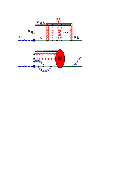
Figure 1: The amplitude $W$ including FSIs between re-scattered eikonalized quark and antiquark. The FSIs are described by a non-perturbative scattering amplitude $\mathrm{M}$ that is calculated in a generalized ladder approximation. Gluon interactions as shown in the second diagram are not taken into account (see text).

We model (7) by the diagram shown in Fig. 1, where the FSIs – generated by the gauge link in (7) – are described by a non-perturbative amputated scattering amplitude $({\mathrm{M}})_{\gamma\delta}^{\alpha\beta}$ with $\beta,\,\alpha$ ($\gamma,\,\delta$) color indices of incoming and outgoing quark (antiquark). In the next section we calculate the scattering amplitude using non-perturbative eikonal methods thereby considering a subclass of possible diagrams with interactions between quark and antiquark. We neglect classes of gluon exchanges in the second diagram in Fig. 1 represented by the red rungs since they would be attributed to the “interaction” between the quark fields and the operator $I$ in (2) and lead to terms which break the relation (5). We also neglect real gluon emission and (self)-interactions of quark and antiquark lines the second diagram in Fig. 1 since they represent radiative corrections of the GPD and are effectively modeled in terms of spectator masses and a phenomenological vertex function.

The pion-quark vertex is modeled with the interaction Lagrangian

$$\mathcal{L}=-\frac{g_{\pi}}{\sqrt{N_{c}}}\delta^{\alpha\beta}\bar{q}^{\alpha}\gamma_{5}\vec{\tau}\cdot\vec{\varphi}q^{\beta},$$ (8)

where we allow the coupling $g_{\pi}$ to depend on the momentum of the active quark in order to take into account the compositeness of the hadron and to suppress large quark virtualities [73, 42, 43]. Applying the Feynman rules we obtain an expression for the matrix element $W$ in (7) from the first diagram in Fig. 1

$$W_{i,\sigma}^{\alpha\beta}(P,k) = \frac{-i\tau}{\sqrt{N_{c}}}\Bigg{[}\delta^{\alpha\beta}g_{\pi}(k^{2})\frac{\left[(\hbox to0.0pt{\hbox to5.52084pt{\hfil/\hfil}\hss}k+m_{q})v(P_{s},\sigma)\right]_{i}}{k^{2}-m_{q}^{2}+i0}+\int\frac{d^{4}q}{(2\pi)^{4}}$$ (9)

$$\frac{g_{\pi}\left((P-q)^{2}\right)\left[(\hbox to0.0pt{\hbox to7.80904pt{\hfil/\hfil}\hss}P-\hbox to0.0pt{\hbox to5.00002pt{\hfil$q$\hfil}\hss}/+m_{q})\gamma_{5}(\hbox to0.0pt{\hbox to5.00002pt{\hfil$q$\hfil}\hss}/-m_{s})\left({\mathrm{M}}\right)_{\delta\beta}^{\alpha\delta}(q,P_{s})v(P_{s},\sigma)\right]_{i}}{\left[n\cdot(P_{s}-q)+i0\right]\left[(P-q)^{2}-m_{q}^{2}+i0\right]\left[q^{2}-m_{s}^{2}+i0\right]}\Bigg{]},$$

where $P_{s}\equiv P-k$ is the spectator momentum. The first term in (9) represents the contribution without FSIs while the second term corresponds to the first diagram in Fig. 1. We then express the FSIs through the amputated quark - antiquark scattering amplitude ${\mathrm{M}}$. Here both incoming quark and antiquark are subject to the eikonal approximation (see, e.g. [74] and references therein). While the active quark undergoes a natural eikonalization for a massless fermion since it represents the gauge link contribution, the eikonalization for a massive spectator fermion is a simplification that is justified by the physical picture of partons in an infinite momentum frame. The eikonalization of a massive fermion can be traced back to the Nordsieck-Bloch approximation [75] which describes a highly energetic helicity conserving fermion undergoing multiple scattering with very small momentum transfer. In this approximation the Dirac vertex structure $\bar{u}(p_{1})\gamma^{\mu}u(p_{2})\sim p_{\mu}/m\equiv v_{\mu}$ where $(p_{1}+p_{2})/2\equiv p$. For a massive anti-fermion one identifies the velocity $v^{\mu}=-p^{\mu}/m$, and the numerator of a fermion propagator becomes $i(-\hbox to0.0pt{\hbox to5.03125pt{\hfil/\hfil}\hss}p+m)\rightarrow i(-v\cdot p+m)$.

We proceed by performing a contour-integration of the light-cone loop-momentum $q^{-}$ in Eq. (9) where we consider poles which originate from the denominators in (9). This assumes that the scattering amplitude ${\mathrm{M}}$ does not contain poles in $q^{-}$ and the integrand is well behaved on the contour in $q^{-}$. Before we proceed, it is important to point out that one-loop calculations of T-odd functions were performed in a scalar diquark model [33, 35, 38] and a quark target model [76] where there are no contributions from a pole in $q^{-}$ in the exchanged gluon propagator. This is one reason why a factorization of the form (5) is exact in the one gluon exchange approximation. One does not expect this feature to hold in higher order calculations. In fact when including axial-vector diquarks [42] in the one-gluon exchange approximation a $q^{-}$ pole contribution from the exchanged gluon exists which leads to light-cone divergences when $q^{-}\rightarrow\infty$ and $q^{+}\rightarrow 0$. An introduction of a slightly off-light-like vector $\upsilon$ regulates this divergence resulting in logarithmic dependence of the form, $\rm{log}(\upsilon^{+}/\upsilon^{-})$ [77]. Such logarithmic terms prevent a factorization of the form (5). Alternatively, one may introduce certain vertex function $g_{\pi}(k^{2})$ by hand that suppress contributions from $q^{-}$ - poles [42]. Performing the contour integration on $q^{-}$ under these assumptions fixes the momentum $q^{-}$ of the antiquark in the loop in (9) to $q^{-}=(\vec{q}_{T}^{2}+m_{s}^{2})/2q^{+}$.

The eikonal propagator can be split into a real and imaginary part using $1/(x+i0)=\mathcal{P}(1/x)-i\pi\delta(x)$. It has been argued in [46] that only the imaginary part contributes to the relation (5) as it forces the antiquark momentum $q$ to be on the mass shell. Thus, the imaginary part of the eikonal propagator corresponds to a cut of the first diagram in Fig. 1. From the point of view of FSIs, the kinematical point $q^{+}=(1-x)P^{+}$ is the ’natural’ choice for the plus component of the spectator. In the picture where one imagines the scattered quark and antiquark to move quasi-collinearly with respect to the target pion – backwards and forwards respectively – the quark and antiquark exchange soft gluons. Under these kinematic condition one would expect the FSIs to be dominated by the “small” transverse momenta of quark and antiquark rather than the “large” plus momenta. An integration over $q^{+}$ in (LABEL:eq:Wi2) where contributions other than the pole term contribute include configurations where large momentum is also transferred from quark to antiquark in the plus direction. Nevertheless the principle value does contribute to the integral (LABEL:eq:Wi2) which allows for such momentum configurations. While this effect is beyond the picture of FSIs from soft gluon exchange, we will consider this in a future publication. Proceeding with the picture of soft gluon exchange there is a clean separation of FSIs and spatial distortion of the parton distribution in the transverse plane in the sense of (5). Using only the imaginary part of the eikonal propagator Eq. (9) reduces to

$$W_{i,\sigma}^{\alpha\beta}(P,k) = \frac{i\tau}{\sqrt{N_{c}}}(1-x)\Bigg{[}\delta^{\alpha\beta}g_{\pi}(k^{2})\frac{\left[(\hbox to0.0pt{\hbox to5.52084pt{\hfil/\hfil}\hss}k+m_{q})\gamma_{5}v(P_{s},\sigma)\right]_{i}}{\vec{k}_{T}^{2}+\tilde{m}^{2}}+$$

$$\int\frac{d^{2}q_{T}}{(2\pi)^{2}}\frac{g_{\pi}\left((P-q)^{2}\right)\left[(\hbox to0.0pt{\hbox to7.80904pt{\hfil/\hfil}\hss}P-\hbox to0.0pt{\hbox to5.00002pt{\hfil$q$\hfil}\hss}/+m_{q})\gamma_{5}v(P_{s},\sigma)\right]_{i}\left(\bar{{\mathrm{M}}}\right)_{\delta\beta}^{\alpha\delta}(q;P_{s})}{\left[\vec{q}_{T}^{2}+\tilde{m}^{2}\right]}\Bigg{]}.$$

We have introduced the notation $\bar{{\mathrm{M}}}=m_{s}\mathrm{M}/(2(1-x)P^{+})$.

Now we use (LABEL:eq:Wi2) to calculate the pion Boer-Mulders function via (6). Specifying the pion-quark-antiquark vertex function

$$g_{\pi}(k^{2})=g_{\pi}\frac{(-\Lambda^{2})^{n-1}}{(n-1)!}\partial_{\Lambda^{2}}^{n-1}\frac{(k^{2}-m_{q}^{2})f(k^{2})}{k^{2}-\Lambda^{2}+i0},$$ (11)

where $f$ is a homogeneous function of the quark virtuality, we choose it to be a Gaussian $\exp[-\lambda^{2}|k^{2}|]$ in accordance with Ref. [42]. Inserting (LABEL:eq:Wi2) into (6) and a bit of algebra yields the following expression for the Boer-Mulders function

$$\epsilon_{T}^{ij}k_{T}^{j}h_{1}^{\perp}(x,\vec{k}_{T}^{2}) = \frac{2g_{\pi}^{2}m_{\pi}}{(2\pi)^{3}\Lambda^{2}}(xm_{s}+(1-x)m_{q})\left((1-x)\Lambda^{2}\right)^{2n-1}$$ (12)

$$\times\int\frac{d^{2}q_{T}}{(2\pi)^{2}}\frac{d^{2}p_{T}}{(2\pi)^{2}}\,\epsilon_{T}^{ji}(q_{T}^{j}-p_{T}^{j})\frac{\mathrm{e}^{-\frac{2\lambda^{2}}{1-x}(xm_{s}^{2}-x(1-x)m_{\pi}^{2})}\mathrm{e^{-\frac{\lambda^{2}}{1-x}(\vec{q}_{T}^{2}+\vec{p}_{T}^{2})}}}{\left[\vec{q}_{T}^{2}+\tilde{\Lambda}^{2}(x)\right]^{n}\left[\vec{p}_{T}^{2}+\tilde{\Lambda}^{2}(x)\right]^{n}}$$

$$\times\left(\Im[{\bar{\mathrm{M}}}^{\mathrm{eik}}]\right)_{\delta\beta}^{\alpha\delta}(\vec{k}_{T}+\vec{q}_{T})\Big{(}(2\pi)^{2}\delta^{\alpha\beta}\delta^{(2)}(\vec{p}_{T}+\vec{k}_{T})$$

$$\hskip 56.9055pt+\left(\Re[\bar{{\mathrm{M}}}^{\mathrm{eik}}]\right)_{\gamma\alpha}^{\beta\gamma}(\vec{k}_{T}+\vec{p}_{T})\Big{)},$$

with $\tilde{\Lambda}^{2}(x)=xm_{s}^{2}-x(1-x)m_{\pi}^{2}+(1-x)\Lambda^{2}$. Anticipating an eikonal form for the scattering amplitude $\bar{{\mathrm{M}}}(x,\vec{k}_{T},\vec{q}_{T})\rightarrow\bar{{\mathrm{M}}}^{\mathrm{eik}}(|\vec{q}_{T}+\vec{k}_{T}|)$ that will be discussed in the next section we exploit this property to simplify the expression and show a relation to the chirally-odd GPD $H_{1}^{\pi}$. Since GPDs are defined from collinear light-cone correlations functions gauge link contributions to GPDs don’t lead to an observable effect. In fact, in light-cone gauge the corresponding contributions from the gauge link are re-shuffled into the gluon propagators [35] and they appear as gluon dressings of the tree-level contribution to GPDs. Thus one can consistently describe GPDs from tree-level diagrams in the spectator model where the effects of gluon dressings are effectively hidden in the model parameters. A calculation for the GPD $H_{1}^{\pi}$ for an antiquark spectator can be found in [48]. It is easy to generalize it with a phenomenological vertex function (11). We obtain the following representation

$$H_{1}^{\pi}(x,0,-\vec{\Delta}_{T}^{2}) = \frac{-g_{\pi}^{2}m_{\pi}}{2(2\pi)^{3}\Lambda^{2}}(xm_{s}+(1-x)\ m_{q})\left(\frac{(1-x)\Lambda^{2}}{\vec{D}_{T}^{2}+\tilde{\Lambda}^{2}(x)}\right)^{2n-1}$$ (13)

$$\times\int_{0}^{2\pi}d\varphi\int_{0}^{1}dz\frac{z^{2n-2}\mathrm{e}^{2\lambda^{2}\Lambda^{2}}\mathrm{e}^{-\frac{2\lambda^{2}(\vec{D}_{T}^{2}+\tilde{\Lambda}^{2}(x))}{(1-x)z}}}{\left[1-4z(1-z)\frac{\vec{D}_{T}^{2}}{\vec{D}_{T}^{2}+\tilde{\Lambda}^{2}(x)}\cos^{2}\varphi\right]^{n}},$$

where $\vec{D}_{T}^{2}=\frac{1}{4}(1-x)^{2}\vec{\Delta}_{T}^{2}$. Performing a translation of the integration variables in (12) according to $q_{T}\rightarrow q_{T}+k_{T}$ and $p_{T}\rightarrow p_{T}+k_{T}$, a rotation of the form $q_{T}^{\prime}=q_{T}-p_{T}$, $p_{T}^{\prime}=q_{T}+p_{T}$, weighting with a transverse quark vector $k_{T}^{i}$ and integrating both sides over $k_{T}$ we find the relation

$$m_{\pi}^{2}h_{1}^{\perp(1)}(x) = \int\frac{d^{2}q_{T}}{2(2\pi)^{2}}\,\vec{q}_{T}\cdot\vec{I}(x,\vec{q}_{T})H_{1}^{\pi}\left(x,0,-\left(\frac{\vec{q}_{T}}{1-x}\right)^{2}\right)\,.$$ (14)

The function $I^{i}$ can be expressed in terms of the real and imaginary part of the scattering amplitude $\bar{{\mathrm{M}}}$,

$$I^{i}(x,\vec{q}_{T}) = \frac{1}{N_{c}}\int\frac{d^{2}p_{T}}{(2\pi)^{2}}\,(2p_{T}-q_{T})^{i}\,\left(\Im[\bar{{\mathrm{M}}}^{\mathrm{eik}}]\right)_{\delta\beta}^{\alpha\delta}(|\vec{p}_{T}|)$$ (15)

$$\Big{(}(2\pi)^{2}\delta^{\alpha\beta}\delta^{(2)}(\vec{p}_{T}-\vec{q}_{T})+\left(\Re[\bar{{\mathrm{M}}}^{\mathrm{eik}}]\Big{)}_{\gamma\alpha}^{\beta\gamma}(|\vec{p}_{T}-\vec{q}_{T}|)\right).$$

In order to derive the relation (5) one transforms Eq. (14) into the impact parameter space via a Fourier transforms of the following form,

$$\mathcal{H}_{1}^{\pi}(x,\vec{b}_{T}^{2})=\int\frac{d^{2}\Delta_{T}}{(2\pi)^{2}}\,\mathrm{e}^{-i\vec{\Delta}_{T}\cdot\vec{b}_{T}}H_{1}^{\pi}(x,0,-\vec{\Delta}_{T}^{2}).$$ (16)

The lensing function in the impact parameter space then reads,

$$\mathcal{I}^{i}(x,\vec{b}_{T}) = i(1-x)\int\frac{d^{2}q_{T}}{(2\pi)^{2}}\,\mathrm{e}^{i\frac{\vec{q}_{T}\cdot\vec{b}_{T}}{1-x}}I^{i}(x,\vec{q}_{T}).$$ (17)

In the following section we will use a quark-antiquark scattering amplitude computed in relativistic eikonal models as input for the lensing function (15).

4 The Lensing Function in Relativistic Eikonal Model

In order to calculate the 2 $\rightarrow$ 2 scattering amplitude $\mathrm{M}$ (needed for (15)) we use functional methods to incorporate the color degrees of freedom in the eikonal limit when soft gauge bosons couple to highly energetic matter particles on the light cone. It is non-trivial to extend the functional methods established in an Abelian to non-Abelian gauge theory such as QCD. Attempts in this direction were made in Refs. [78, 71], and only recently a fully Lorentz and gauge invariant treatment was presented in Ref. [79]. Here we outline the details of the functional approach as it pertains to implementing color structure to the scattering amplitude $\mathrm{M}$ and thereby the lensing function. We leave the details to a forthcoming publication [80].

Starting from the generating functional $Z$ for QCD in a covariant gauge, a quark antiquark 4-point function $T$ can then be defined by functional derivatives with respect to quark sources which yields,

$$T_{2\rightarrow 2} \propto \int\mathcal{D}A\,\mathrm{e}^{-\frac{i}{4}\int(F^{2}+2\lambda(\partial\cdot A)^{2})}\,\mathrm{e}^{\mathrm{Tr}\ln G^{-1}[A]+\mathrm{Tr}\ln H^{-1}[A]}\,G[A]\,\bar{G}[A].$$

The first exponential describes the gluonic part of the theory including self-interactions and the second exponential describes internal closed quark and ghost loops. $G$, $\bar{G}$ are the non-perturbative quark- and antiquark-propagator determining the external legs of the 4-point function $T$, and $H$ is the ghost propagator [80]. One imposes eikonal approximations on these propagators [70, 71] that simplify the computation of the path-integral. In an Abelian theory the eikonal approximation as discussed in the previous section leads to a well-known eikonal representation [70], which was argued in [78, 71] to generalize to QCD in the following way, e.g. for a massless fermion

$$G_{\alpha\beta}^{\mathrm{eik}}(x,y|A) = -i\int_{0}^{\infty}ds\delta^{(4)}(x-y-sn)\left(\mathrm{e}^{-ig\int_{0}^{s}d\beta\,n\cdot A^{a}(y+\beta n)t^{a}}\right)_{\alpha\beta}^{+},$$

where color is implemented by a path-ordered exponential indicated by the brackets $(...)^{+}$ and the color matrix $t^{a}$ in the exponential.

Inserting the eikonal representation for the quark- and antiquark propagator into Eq. (LABEL:eq:4-pointstart) and implementing the generalized ladder approximation one finds the color gauge invariant result corresponding to the picture of FSIs discussed in the previous section,

$$\left({\mathrm{M}}^{\mathrm{eik}}\right)_{\delta\beta}^{\alpha\delta}(x,|\vec{q}_{T}+\vec{k}_{T}|) = \frac{(1-x)P^{+}}{m_{s}}\int d^{2}z_{T}\,\mathrm{e}^{-i\vec{z}_{T}\cdot(\vec{q}_{T}+\vec{k}_{T})}$$

$$\times\Bigg{[}\int d^{N_{c}^{2}-1}\alpha\int\frac{d^{N_{c}^{2}-1}u}{(2\pi)^{N_{c}^{2}-1}}\,\mathrm{e}^{-i\alpha\cdot u}\left(\mathrm{e}^{i\chi(|\vec{z}_{T}|)t\cdot\alpha}\right)_{\alpha\delta}\left(\mathrm{e}^{it\cdot u}\right)_{\delta\beta}-\delta_{\alpha\beta}\Bigg{]}.$$

In this expression, the ($N_{c}^{2}-1$) dimensional integrals result from auxiliary fields $\alpha^{a}(s)$ and $u^{a}(s)$ that were introduced in the functional formalism (see Ref. [71]) to separate the physical gluon fields from the color matrices. The eikonal phase $\chi(|\vec{z}_{T}|)$ in Eq. (4) represents the arbitrary amount of soft gluon exchanges that are summed up into an exponential form and is expressed in terms of the gluon propagator in a covariant gauge,

$$\chi(|\vec{z}_{T}|)=g^{2}\int_{-\infty}^{\infty}d\alpha\int_{-\infty}^{\infty}d\beta\,n^{\mu}\bar{n}^{\nu}\mathcal{D}_{\mu\nu}(z+\alpha n-\beta\bar{n}),$$ (21)

where $\mathcal{D}$ denotes the gluon propagator, and $g$ is the strong coupling. In this form the 4-velocity vector $v^{\mu}$ is expressed in terms of the complementary light cone vector $\bar{n}$ where $v=-\frac{(1-x)P^{+}}{m_{s}}\bar{n}$, with $n\cdot\bar{n}=1$ and $\bar{n}^{2}=0$. One may choose $\bar{n}=(0,1,\vec{0}_{T})$.

In Eq. (4) we evaluate the color integral,

$$f_{\alpha\beta}(\chi) \equiv \int d^{N_{c}^{2}-1}\alpha\int\frac{d^{N_{c}^{2}-1}u}{(2\pi)^{N_{c}^{2}-1}}\,\mathrm{e}^{-i\alpha\cdot u}\left(\mathrm{e}^{i\chi(|\vec{z}_{T}|)t\cdot\alpha}\right)_{\alpha\delta}\left(\mathrm{e}^{it\cdot u}\right)_{\delta\beta}-\delta_{\alpha\beta}$$

by deriving a power series representation for arbitrary $N_{c}$. We expand the exponential $\exp[i\chi t\cdot\alpha]$ and rewrite the resulting factors as derivatives with respect to $u$. Then we perform integrations by parts which reduces the $\alpha$ integral to a simple $\delta$-function. This simplifies the $u$-integral where $u$ is set to zero after differentiation We obtain

$$f_{\alpha\beta}(\chi)=\sum_{n=1}^{\infty}\frac{(i\chi)^{n}}{n!}(-i)^{n}(t^{a_{1}}...t^{a_{n}})_{\alpha\delta}\frac{\partial^{n}(\mathrm{e}^{it\cdot u})_{\delta\beta}}{\partial u^{a_{1}}...\partial u^{a_{n}}}\Big{|}_{u=0}.$$ (23)

Now we expand the remaining exponential in Eq. (23) and note that one can write the set of partial derivatives with respect to $u^{a_{i}}$ as a sum over all permutations $P_{n}$ of the set $\{1,...,n\}$, which results in the power series representation for $f$,

$$f_{\alpha\beta}(\chi) = \sum_{n=1}^{\infty}\frac{(i\chi)^{n}}{(n!)^{2}}\sum_{a_{1}=1}^{N_{c}^{2}-1}...\sum_{a_{n}=1}^{N_{c}^{2}-1}\sum_{P_{n}}\left(t^{a_{1}}...t^{a_{n}}t^{a_{P_{n}(1)}}...t^{a_{P_{n}(n)}}\right)_{\alpha\beta}.$$ (24)

This color factor matrix nicely illustrates the generalized ladder approximation. If only direct ladder gluons were considered the sum over permutations would become trivial in Eq. (24) and only terms $(t^{a_{1}}...t^{a_{n}}t^{a_{n}}...t^{a_{1}})_{\alpha\beta}=C_{F}^{n}\delta_{\alpha\beta}$ with $C_{F}=\frac{N_{c}^{2}-1}{2N_{c}}$ would contribute. This constitutes the leading order in a large-$N_{c}$ expansion while non-planar diagrams, i.e. crossed gluon graphs, are suppressed. For the leading contribution one may simply replace $\alpha\rightarrow C_{F}\alpha_{s}$ and work in an Abelian theory. In particular, this replacement was suggested in perturbative model calculations [32, 81]. Since we take into account crossed gluons we have to sum over all permutations in (24), and such a replacement is not possible. In an Abelian theory, the generating matrices $t$ reduce to unity, $t=1$, and since we have $n!$ permutations of the set $\{1,...,n\}$, we recover the well-known result for the Coulomb phase,

$$f^{U(1)}(\chi)=\sum_{n=1}^{\infty}\frac{(i\chi)^{n}}{n!}=\mathrm{e}^{i\chi}-1.$$ (25)

For the non-Abelian $N_{c}=2$ theory the generators are given by the Pauli matrices $\sigma^{a}=2t^{a}$. Instead of using the power series representation we can calculate the integral (LABEL:eq:ColorIntegral) analytically by means of the relation $\left(\mathrm{e}^{iu\cdot\frac{\sigma}{2}}\right)_{\alpha\beta}=\delta_{\alpha\beta}\cos\left(\frac{|u|}{2}\right)+\frac{i\vec{\sigma}_{\alpha\beta}\cdot\vec{u}}{|u|}\sin\left(\frac{|u|}{2}\right)$. We obtain a slightly different result compared to Ref. [71] for SU(2),

$$f_{\alpha\beta}^{SU(2)}(\frac{\chi}{4}) = \delta_{\alpha\beta}\left(\cos\frac{\chi}{4}-\frac{\chi}{4}\sin\frac{\chi}{4}-1+i\left(2\sin\frac{\chi}{4}+\frac{\chi}{4}\cos\frac{\chi}{4}\right)\right).$$

As a check on our numerical and analytical approaches we numerically calculate the lowest coefficients in the power series (24), and they agree with the coefficients in an expansion in $\chi$ of the analytical result (LABEL:eq:SU2Analytical). The disadvantage of using the power series representation (24) is apparent for numerical calculations since the number of operations grows with $n!$. That said, for SU(2) we calculated the first eight coefficients. For QCD, $N_{c}=3$, the generators $t$ are given by the Gell-Mann matrices $\lambda^{a}=2t^{a}$. Due to the difficulty of integrating over the Haar measure in Eq. (LABEL:eq:ColorIntegral) we put off the analytical treatment [80]. Using the power series (24) we derive the following approximative color function for $a=\chi/4$

$$\Re[f_{\alpha\beta}^{SU(3)}](a) = \delta_{\alpha\beta}(-c_{2}a^{2}+c_{4}a^{4}-c_{6}a^{6}-c_{8}a^{8}+...),$$

$$\Im[f_{\alpha\beta}^{SU(3)}](a) = \delta_{\alpha\beta}(c_{1}a-c_{3}a^{3}+c_{5}a^{5}-c_{7}a^{7}+...),$$ (27)

with the numerical values $c_{1}=5.333$, $c_{2}=6.222$, $c_{3}=3.951$, $c_{4}=1.934$, $c_{5}=0.680$, $c_{6}=0.198$, $c_{7}=0.047$, $c_{8}=0.00967$.

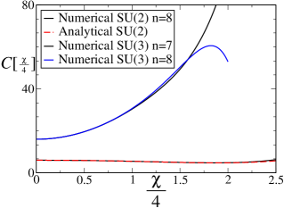
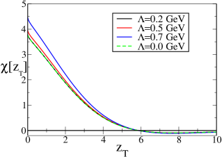
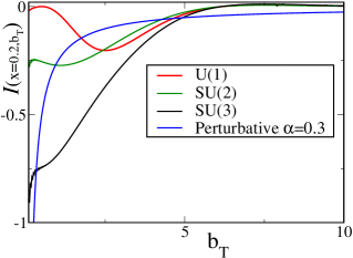
Figure 2: Left: $C[\frac{\chi}{4}]$ of Eq. (30) as a function of the eikonal amplitude $\frac{\chi}{4}$. We compare the numerical result computed by means of Eq. (24) up to the order $n=8$ with the analytical result in Eq. (4) for the $SU(2)$ color case. The numerical and analytical result agree up to $\frac{\chi}{4}\sim 2$. For $SU(3)$, we compare the numerical results for the orders $n\,=7,\,8$. The results are reliable for $\frac{\chi}{4}\sim 1.5$. Center: The eikonal phase $\chi^{DS}(|\vec{z}_{T}|)$ vs. $|\vec{z}_{T}|$ with input from Dyson-Schwinger equations at scales $\Lambda_{QCD}=0\,\mathrm{GeV},\,0.2\,\mathrm{GeV},\,0.5\,\mathrm{GeV},\,0.7\,\mathrm{GeV}$. Right: The lensing function $\mathcal{I}^{i}(x,\vec{b}_{T})$ from Eq. (4) for U(1), SU(2) and SU(3) for $x=0.2$ at a scale $\Lambda_{QCD}=0.2\,\mathrm{GeV}$. For comparison we also plot the perturbative result of Ref. [48] including the eikonalized antiquark spectator with an arbitrary value for the coupling, $\alpha=0.3$.

Working in coordinate space we express the lensing function directly in terms of the eikonal phase $\chi$ defined in Eq. (21). Defining the eikonal amplitude as in section 3, where the real and imaginary part are

$$\Re[\bar{{\mathrm{M}}}_{\alpha\beta}](\vec{p)} = \frac{1}{2}\int d^{2}z\,\mathrm{e}^{i\vec{p}\cdot\vec{z}}\Re[f_{\alpha\beta}(\chi(|\vec{z}_{T}|))],$$ (28)

$$\Im[\bar{{\mathrm{M}}}_{\alpha\beta}](\vec{p}) = \frac{1}{2}\int d^{2}z\,\mathrm{e}^{i\vec{p}\cdot\vec{z}}\Im[f_{\alpha\beta}(\chi(|\vec{z}_{T}|))],$$ (29)

we insert (28) and (29) into the lensing function (15) then transform it via (17) into the impact parameter space. This yields a lensing function of the form,

$$\mathcal{I}^{i}(x,\vec{b}_{T}) = \frac{(1-x)}{2N_{c}}\frac{b_{T}^{i}}{|\vec{b}_{T}|}\frac{\chi^{\prime}}{4}C[\frac{\chi}{4}],$$

$$C[\frac{\chi}{4}] \equiv \Bigg{[}\left(\mathrm{Tr}\Im[f]\right)^{\prime}(\frac{\chi}{4})+\frac{1}{2}\mathrm{Tr}\left[\left(\Im[f]\right)^{\prime}(\frac{\chi}{4})\left(\Re[f]\right)(\frac{\chi}{4})\right]$$ (30)

$$-\frac{1}{2}\mathrm{Tr}\left[\left(\Im[f]\right)(\frac{\chi}{4})\left(\Re[f]\right)^{\prime}(\frac{\chi}{4})\right]\Bigg{]},$$

where $\chi^{\prime}$ denotes the first derivative with respect to $|\vec{z}_{T}|$, and $\left(\Im[f]\right)^{\prime}$ and $\left(\Re[f]\right)^{\prime}$ are the first derivatives of the real and imaginary parts of the color function $f$. Also, the eikonal phase is understood to be a function of $|\vec{b}_{T}|/(1-x)$. Inserting (25) into (4) results into the following expression for the lensing function in an Abelian U(1)-theory

$$\mathcal{I}_{U(1)}^{i}(x,\vec{b}_{T}) = (1-x)\frac{b_{T}^{i}}{4|\vec{b}_{T}|}\chi^{\prime}(\frac{|\vec{b}_{T}|}{1-x})\left(1+\cos\chi(\frac{|\vec{b}_{T}|}{1-x})\right).$$ (31)

Similarly from (LABEL:eq:SU2Analytical) we calculate the lensing function in an SU(2)-theory

$$\mathcal{I}_{SU(2)}^{i}(x,\vec{b}_{T}) = \frac{(1-x)b_{T}^{i}}{16|\vec{b}_{T}|}\chi^{\prime}(\frac{|\vec{b}_{T}|}{1-x})$$

$$\times\Bigg{(}3(1+\cos\frac{\chi}{4})+\left(\frac{\chi}{4}\right)^{2}-\sin\frac{\chi}{4}\left(\frac{\chi}{4}-\sin\frac{\chi}{4}\right)\Bigg{)}\Big{|}_{\chi=\chi\left(\frac{|\vec{b}_{T}|}{1-x}\right)}.$$

For the SU(3)-QCD case we use Eq. (27). In Fig. 2 the function $C[\frac{\chi}{4}]$ is plotted versus $\frac{\chi}{4}$. While the convergence of the power series is slightly better for SU(2) where the numerical result, calculated to eighth order, agrees with the analytical result up to $\frac{\chi}{4}\sim 2$, we can trust the numerical result computed with eight coefficients up to $\frac{\chi}{4}\sim 1.5$ for SU(3).

At this point we discuss the eikonal phase $\chi$ as defined in (21) which is determined by two quantities, the strong coupling $g$ and the gluon propagator $\mathcal{D}$. One can write a general form for the gluon propagator in momentum space

$$\mathcal{D}_{\mu\nu}^{ab}(z) = \delta^{ab}\int\frac{d^{4}k}{(2\pi)^{4}}\,\tilde{\mathcal{D}}_{\mu\nu}(k)\mathrm{e}^{-ik\cdot z}$$ (33)

$$\equiv \delta^{ab}\int\frac{d^{4}k}{(2\pi)^{4}}\,\left[g_{\mu\nu}\tilde{\mathcal{D}}_{1}(k^{2})+k_{\mu}k_{\nu}\tilde{\mathcal{D}}_{2}(k^{2})\right]\mathrm{e}^{-ik\cdot z},$$

where the gauge dependent part is in $\tilde{\mathcal{D}}_{2}$. However, the gauge dependent part does not appear in the eikonal phase when inserting Eq. (33) into Eq. (21) because the eikonal vectors $n$ and $v\simeq-\frac{(1-x)P^{+}}{m_{s}}\bar{n}$ are light-like. Performing the integral yields the following expression for the eikonal phase

$$\chi(|\vec{z}_{T}|)=\frac{g^{2}}{2\pi}\int_{0}^{\infty}dk_{T}\,k_{T}\,J_{0}(|\vec{z}_{T}|k_{T})\tilde{\mathcal{D}}_{1}(-k_{T}^{2}),$$ (34)

where $J_{0}$ is a Bessel function of the first kind. The gluon propagator represents all exponentiated gluons exchanged between the two eikonal lines in the generalized ladder approximation in Fig. 1. The couplings represent the strength of the quark (antiquark) - gluon interaction in Fig. 1.

As a check of the calculation we investigated the perturbative limit of our calculation. Assuming that the quark - gluon interaction $g^{2}$ is small and using perturbative gluon propagator in Feynman gauge for $\tilde{\mathcal{D}}_{1}$ one can expand our non-perturbative result in Eq. (30) to $g^{2}$. The leading order corresponds to the result of the one-loop calculation of the Boer-Mulders function of Ref. [48] after additional eikonalization of the antiquark.

5 Non-perturbative Quantities from the Dyson-Schwinger approach

In order to obtain a numerical estimate for the eikonal phase, it is important to have a realistic estimate of the size of the QCD coupling $g$ or $\alpha_{s}=\frac{g^{2}}{4\pi}$. Since all the gluons exchanges between the eikonal lines are soft, the interactions take place at a soft scale. Thus we need to know the running of the strong coupling in the infrared limit. Inserting a perturbative gluon propagator might not describe the gluon exchange realistically. One would expect that a non-perturbative gluon propagator would be a better choice. The infrared behavior of both quantities, the running of the strong coupling and the non-perturbative gluon propagator, have been studied in the framework of the Dyson-Schwinger equations [82, 83, 84, 85] and also in lattice(see e.g. [86]). One learns from such studies that the strong coupling has a value of about $\alpha_{s}(0)\simeq 2.972$ in the infrared limit. In particular in Ref. [82] fits were presented for the running coupling. Since we are merely interested in a numerical estimate of the lensing function we will apply the simplest form of the running coupling presented in [82],

$$\alpha_{s}(\mu^{2})=\frac{\alpha_{s}(0)}{\ln\left[\mathrm{e+a_{1}(\mu^{2}/\Lambda^{2})^{a_{2}}+b_{1}(\mu^{2}/\Lambda^{2})^{b_{2}}}\right]}.$$ (35)

The values for the fit parameters are $\Lambda=0.71\,\mathrm{GeV}$, $a_{1}=1.106$, $a_{2}=2.324$, $b_{1}=0.004$ and $b_{2}=3.169$. These calculations were performed in Euclidean space where Landau gauge was applied, and agree reasonably well with each other. Because the light cone components in Eq. (34) are already integrated out and the remaining integration range is over a 2-dimensional transverse Euclidean space, and because the gauge dependent part of the gluon propagator does not contribute, it is natural to apply the Euclidean results in Landau gauge of the Dyson-Schwinger framework. One unique feature of Dyson-Schwinger studies of the gluon propagator is that it rises like $(k^{2})^{2\kappa-1}$ in the infra-red limit with a universal coefficient $\kappa\simeq 0.595$. This makes it infrared finite in contrast to the perturbative propagator. A fit to the results for the non-perturbative gluon propagator has been given in Ref. [87, 82, 88],

$$Z(p^{2},\mu^{2}) \,=\, p^{2}\mathcal{D}^{-1}(p^{2},\mu^{2})$$ (36)

$$=\left(\frac{\alpha_{s}(p^{2})}{\alpha_{s}(\mu^{2})}\right)^{1+2\delta}\left(\frac{c\left(\frac{p^{2}}{\Lambda^{2}}\right)^{\kappa}+d\left(\frac{p^{2}}{\Lambda^{2}}\right)^{2\kappa}}{1+c\left(\frac{p^{2}}{\Lambda^{2}}\right)^{\kappa}+d\left(\frac{p^{2}}{\Lambda^{2}}\right)^{2\kappa}}\right)^{2},$$

with the parameters $c=1.269$, $d=2.105$, and $\delta=-\frac{9}{44}$. These fits for the running coupling and the gluon propagator merge with the spirit of the eikonal methods described above since closed fermion loops (quenched approximation) were neglected. By using the non-perturbative propagator (36), we partly reintroduce gluon self-interactions that were originally neglected in the generalized ladder approximation. According to Ref. [88] the fitting functions Eqs. (35) and (36) were adjusted to Dyson-Schwinger results obtained at a very large renormalization scale, the mass of the top quark, $\mu^{2}=170\,\mathrm{GeV}^{2}$, which defines the normalization in (36). Since the lensing function deals with soft physics, intuitively we prefer a much lower hadronic scale which sets the normalization, $\mu=\Lambda_{QCD}\approx 0.2\,\mathrm{GeV}$. In the spirit of Sudakov form factors we also assume that the scale at which the gluons are exchanged is given by the transverse gluon momentum that we integrate over. In this way the running coupling serves as a vertex form factor that additional cuts off large gluon transverse momenta.

Our ansatz for the eikonal phase given by Dyson-Schwinger quantities then reads,

$$\chi^{DS}(|\vec{z}_{T}|) = 2\int_{0}^{\infty}dk_{T}\,k_{T}\alpha_{s}(k_{T}^{2})J_{0}(|\vec{z}_{T}|k_{T})Z(k_{T}^{2},\Lambda_{QCD}^{2})/k_{T}^{2}.$$ (37)

The numerical result for this ansatz is shown in the center panel of Fig. 2. We plot this function for various scale $\Lambda_{QCD}=0\,\mathrm{GeV}$, $0.2\,\mathrm{GeV}$, $0.5\,\mathrm{GeV}$, $0.7\,\mathrm{GeV}$. Although the choice of this scale is rather arbitrary we observe only a very mild dependence on this scale as long as it remains soft. We further observe that the phase doesn’t exceed a value of $4$ - $4.5\,\rightarrow\chi_{\mathrm{m}ax}/4\approx 1.15$. Thus this feature makes the application of the power series of the color function in SU(3) reliable since $\chi/4$ never exceeds $1.5$ in the lensing function, Eq. (30) and in turn in the calculation of the Boer-Mulders function in Eq. (5).

Finally, we insert our ansatz for the eikonal phase into the lensing functions (4) for a U(1), SU(2) and SU(3) color function. We plot the results in Fig. 3 for a color function for U(1), SU(2), SU(3). While we observe that all lensing functions fall off at large transverse distances, they are quite different in size at small distances. However for each case, the all order calculation sums up to an exponential of the eikonal phase where one observes oscillations from the Bessel function $J_{0}$ of the first kind. Despite these oscillations the lensing function remains negative.

6 The Pion Boer-Mulders Function

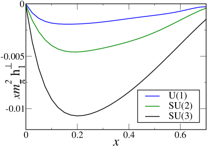
Figure 3: The pion Boer-Mulders function, $xm_{\pi}^{2}h_{1}^{\perp,(1)}(x)$ vs. $x$ calculated by means of the relation to the chirally-odd GPD $\mathcal{H}_{1}^{\pi}$ for a SU(3), SU(2), U(1) gauge theory.

In this section we use the eikonal model for the lensing function together with the spectator model for the GPD $H_{1}^{\pi}$ to present predictions of the relation (5) for the first moment of the pion Boer-Mulders function $h_{1}^{\perp(1)}$.

We start by fixing the model parameters in (13). We encounter six free model parameters $m_{s}$, $m_{q}$, $\Lambda$, $\lambda$, $g_{\pi}$ and $n$ that we need to determine by fitting to pion data. In order to do so we determine the chiral-even GPD $F_{1}^{\pi}$ (for definition and notation see Ref. [48]) in the spectator model,

$$F_{1}^{\pi}(x,0,-\vec{\Delta}_{T}^{2}) = \frac{g_{\pi}^{2}}{2(2\pi)^{2}}\mathrm{e}^{2\lambda^{2}\Lambda^{2}}\left(\frac{(1-x)\Lambda^{2}}{\vec{D}_{T}^{2}+\tilde{\Lambda}^{2}(x)}\right)^{2n-2}$$

$$\times\int_{0}^{2\pi}d\varphi\int_{0}^{1}dz\frac{z^{2n-3}\left[1-2z-z\frac{x(1-x)m_{\pi}^{2}-2m_{s}m_{q}}{\vec{D}_{T}^{2}+\tilde{\Lambda}^{2}(x)}\right]\mathrm{e}^{-\frac{2\lambda^{2}(\vec{D}_{T}^{2}+\tilde{\Lambda}^{2}(x))}{(1-x)z}}}{\left[1-4z(1-z)\frac{\vec{D}_{T}^{2}}{\vec{D}_{T}^{2}+\tilde{\Lambda}^{2}(x)}\cos^{2}\varphi\right]^{n}}.$$

When integrated over $x$, the GPD reduces to the pion form factor $F^{\pi^{+}}(Q^{2})=-F^{\pi^{-}}(Q^{2})$. An experimental fit of the pion form factor to data is presented in Refs. [89, 90], and up to $Q^{2}=2.45\,\mathrm{GeV^{2}}$ is displayed by the monopole formula $F_{\mathrm{fit}}(Q^{2})=(1+1.85\,Q^{2})^{-1}$. This procedure is expected to predict the $t$-dependence of the chirally-odd GPD $H_{1}^{\pi}$ reasonably well up to $Q^{2}=2.45\,\mathrm{GeV^{2}}$. In order to fix the $x$-dependence of $H_{1}^{\pi}$ we fit the collinear limit $F_{1}^{\pi}(x,0,0)$ to the valence quark distribution in a pion. A parameterization for $F_{1}^{\pi}(x)$ was given by GRV in Ref. [91] at a scale $\mu^{2}=2\,\mathrm{GeV^{2}}$. Reasonable agreements of the form factor- and collinear limit of Eq. (6) with the data fits are found for the parameters $m_{q}=0.834\,\mathrm{GeV}$, $m_{s}=0.632\,\mathrm{GeV}$, $\Lambda=0.067\,\mathrm{GeV}$, $\lambda=0.448\,\mathrm{GeV}$, $n=0.971$, $g_{\pi}=3.604$. Details of the fitting procedure for this and an analogous calculation for the Sivers function will be presented in a future publication  [80].

With the predicted GPD $H_{1}^{\pi}$ and the lensing function $\mathcal{I}^{i}(x,\vec{b}_{T})\equiv b_{T}^{i}/|b_{T}|\mathcal{I}(x,|b_{T}|)$ as input we use (5) to give a prediction for the valence contribution to the first $k_{T}$-moment of the pion Boer-Mulders function,

$$m_{\pi}^{2}h_{1}^{\perp(1)}(x)=2\pi\int_{0}^{\infty}db_{T}\,b_{T}^{2}\mathcal{I}(x,b_{T})\frac{\partial}{\partial b_{T}^{2}}\mathcal{H}_{1}^{\pi}(x,b_{T}^{2}).$$ (39)

Numerical results for $m_{\pi}^{2}h_{1}^{\perp(1)}(x)$ are presented in Fig. 3 for a U(1), SU(2) and SU(3) gauge theory. One observes that all results are negative which reflects the sign of the lensing function. It was argued in Ref. [66] that a negative sign of the lensing functions indicates attractive FSIs. We find that this is valid in an Abelian perturbative model as well as our non-perturbative model in a non-Abelian gauge theory. The magnitude of the SU(3) result is about $0.01$, while the SU(2) result and U(1) result are smaller. One observes a growth of the pion Boer-Mulders function with $N_{c}$. Similar growth was also predicted by a model-independent large $N_{c}$ analysis for the nucleon [92], though with different leading order behavior. A phenomenological calculation of the ratio $k_{\perp}h_{1}^{\perp\pi}(x,k_{\perp})/m_{\pi}F_{1}^{\pi}(x,k_{\perp})$ was carried out in a perturbative, Abelian, one gluon exchange approximation and used to estimate the $\cos 2\phi$ AA in $\pi^{-}p$ Drell-Yan scattering [41]. Similar effects were seen as compared to $p\bar{p}$ Drell Yan scattering [93, 94, 95, 96]. It will be useful to study the dependence of the $\cos 2\phi$ AA on color degrees of freedom from this non-perturbative approach. So far the pion Boer-Mulders function is an unknown function but may be accessible from a proposed pion-proton Drell-Yan experiment by the COMPASS collaboration. If a pion Boer-Mulders function is extracted from such an experiment our analysis can be used to quantitatively test the GPD - TMD relation (5). As a comparison, an extraction of another T-odd parton distribution, the proton Sivers function $f_{1T}^{\perp(1)}$, from SIDIS data measured at HERMES and COMPASS [97, 98] reveals an effect of the magnitude of about $0.04$. A similar calculation using eikonal methods for the proton Sivers function will be reported elsewhere [80].

7 Conclusions

In this paper we examined the FSIs of an active quark in a pion which are essential to generate a non-vanishing chirally-odd and (naive) T-odd parton distribution i.e. the Boer-Mulders function. We considered a pion in a valence quark configuration and worked in a spectator framework. The FSIs then were modeled by a non-perturbative 2 $\rightarrow$ 2 scattering amplitude which we calculated using eikonal methods. This treatment sums up all soft gluons between re-scattered quark and antiquark while taking into account color degrees of freedom and leads to a more complete description of FSIs as compared to calculations in the perturbative Abelian one gluon exchange approximation. We find that under the kinematical conditions of soft gluon exchange for FSIs, the Boer-Mulders function can be split into FSIs modeled by eikonal methods and a spatial distribution of quarks in a plane transverse to the direction of motion. This spatial distribution is described by a chirally-odd pion impact parameter GPD which we calculate in the spectator model. Together, both effects, i.e. FSI and spatial distortion give a prediction for the first moment of the Boer-Mulders function that can be tested in pion-proton Drell-Yan experiments.

Acknowledgments

We thank D. Boer, S. Brodsky, M. Burkardt, H. Fried, G. Goldstein, S. Liuti, A. Metz, P.J. Mulders, J.-W. Qiu, O. Teryaev, and H. Weigel for useful discussions. L. G. is grateful for for support from G. Miller and the Institute For Nuclear Theory, University of Washington where part of this work was undertaken. L.G. acknowledges support from U.S. Department of Energy under contract DE-FG02-07ER41460. Authored by Jefferson Science Associates, LLC under U.S. DOE Contract No. DE-AC05-06OR23177. The U.S. Government retains a non-exclusive, paid-up, irrevocable, world-wide license to publish or reproduce this manuscript for U.S. Government purposes.

References

- [1] G. Bunce et al., Phys. Rev. Lett. 36, 1113 (1976).
- [2] W. H. Dragoset et al., Phys. Rev. D18, 3939 (1978).
- [3] J. Antille et al., Phys. Lett. B94, 523 (1980).
- [4] FNAL-E704, D. L. Adams et al., Phys. Lett. B264, 462 (1991).
- [5] COMPASS, C. Schill, Nucl. Phys. Proc. Suppl. 186, 74 (2009).
- [6] HERMES, A. Airapetian et al., Phys. Rev. Lett. 84, 4047 (2000).
- [7] HERMES, A. Airapetian et al., Phys. Rev. Lett. 94, 012002 (2005).
- [8] CLAS, H. Avakian et al., Phys. Rev. D69, 112004 (2004).
- [9] CLAS, H. Avakian, P. E. Bosted, V. Burkert, and L. Elouadrhiri, AIP Conf. Proc. 792, 945 (2005).
- [10] STAR, J. Adams et al., Phys. Rev. Lett. 92, 171801 (2004).
- [11] PHENIX, S. S. Adler et al., Phys. Rev. Lett. 95, 202001 (2005).
- [12] BRAHMS, I. Arsene et al., Phys. Rev. Lett. 101, 042001 (2008).
- [13] STAR, B. I. Abelev et al., Phys. Rev. Lett. 101, 222001 (2008).
- [14] G. L. Kane, J. Pumplin, and W. Repko, Phys. Rev. Lett. 41, 1689 (1978).
- [15] A. V. Efremov and O. V. Teryaev, Phys. Lett. B150, 383 (1985).
- [16] A. V. Efremov and O. V. Teryaev, Sov. J. Nucl. Phys. 36, 140 (1982).
- [17] J.-w. Qiu and G. Sterman, Phys. Rev. Lett. 67, 2264 (1991).
- [18] J.-w. Qiu and G. Sterman, Nucl. Phys. B378, 52 (1992).
- [19] J. P. Ralston and D. E. Soper, Nucl. Phys. B152, 109 (1979).
- [20] R. L. Jaffe and X.-D. Ji, Phys. Rev. Lett. 67, 552 (1991).
- [21] J. C. Collins, Nucl. Phys. B396, 161 (1993).
- [22] D. W. Sivers, Phys. Rev. D41, 83 (1990).
- [23] M. Anselmino, M. Boglione, and F. Murgia, Phys. Lett. B362, 164 (1995).
- [24] P. J. Mulders and R. D. Tangerman, Nucl. Phys. B461, 197 (1996).
- [25] D. Boer and P. J. Mulders, Phys. Rev. D57, 5780 (1998).
- [26] D. Boer, P. J. Mulders, and F. Pijlman, Nucl. Phys. B667, 201 (2003).
- [27] X. Ji, J.-W. Qiu, W. Vogelsang, and F. Yuan, Phys. Rev. Lett. 97, 082002 (2006).
- [28] X. Ji, J.-W. Qiu, W. Vogelsang, and F. Yuan, Phys. Lett. B638, 178 (2006).
- [29] A. Bacchetta, D. Boer, M. Diehl, and P. J. Mulders, JHEP 08, 023 (2008).
- [30] X.-d. Ji, J.-p. Ma, and F. Yuan, Phys. Rev. D71, 034005 (2005).
- [31] D. W. Sivers, Phys. Rev. D43, 261 (1991).
- [32] S. J. Brodsky, D. S. Hwang, and I. Schmidt, Phys. Lett. B530, 99 (2002).
- [33] J. C. Collins, Phys. Lett. B536, 43 (2002).
- [34] A. V. Belitsky, X. Ji, and F. Yuan, Nucl. Phys. B656, 165 (2003).
- [35] X.-d. Ji and F. Yuan, Phys. Lett. B543, 66 (2002).
- [36] G. R. Goldstein and L. Gamberg, (2002), Transversity and meson photoproduction, Proceedings of ICHEP 2002; North Holland, Amsterdam, p. 452 (2003), hep-ph/0209085, Published in Amsterdam ICHEP 452-454.
- [37] D. Boer, S. J. Brodsky, and D. S. Hwang, Phys. Rev. D67, 054003 (2003).
- [38] L. P. Gamberg, G. R. Goldstein, and K. A. Oganessyan, Phys. Rev. D67, 071504 (2003).
- [39] L. P. Gamberg, G. R. Goldstein, and K. A. Oganessyan, Phys. Rev. D68, 051501 (2003).
- [40] A. Bacchetta, A. Schaefer, and J.-J. Yang, Phys. Lett. B578, 109 (2004).
- [41] Z. Lu and B.-Q. Ma, Phys. Rev. D70, 094044 (2004).
- [42] L. P. Gamberg, G. R. Goldstein, and M. Schlegel, Phys. Rev. D77, 094016 (2008).
- [43] A. Bacchetta, F. Conti, and M. Radici, Phys. Rev. D78, 074010 (2008).
- [44] M. Burkardt, Int. J. Mod. Phys. A18, 173 (2003).
- [45] M. Burkardt and D. S. Hwang, Phys. Rev. D69, 074032 (2004).
- [46] S. Meissner, A. Metz, and K. Goeke, Phys. Rev. D76, 034002 (2007).
- [47] A. V. Belitsky, X.-d. Ji, and F. Yuan, Phys. Rev. D69, 074014 (2004).
- [48] S. Meissner, A. Metz, M. Schlegel, and K. Goeke, JHEP 08, 038 (2008).
- [49] QCDSF, D. Brommel et al., Phys. Rev. Lett. 101, 122001 (2008).
- [50] M. Burkardt and B. Hannafious, Phys. Lett. B658, 130 (2008).
- [51] NA10, S. Falciano et al., Z. Phys. C31, 513 (1986).
- [52] NA10, M. Guanziroli et al., Z. Phys. C37, 545 (1988).
- [53] J. S. Conway et al., Phys. Rev. D39, 92 (1989).
- [54] K. Goeke, A. Metz, and M. Schlegel, Phys. Lett. B618, 90 (2005).
- [55] J. C. Collins, D. E. Soper, and G. Sterman, Adv. Ser. Direct. High Energy Phys. 5, 1 (1988).
- [56] A. Bacchetta et al., JHEP 02, 093 (2007).
- [57] X.-d. Ji, J.-P. Ma, and F. Yuan, Phys. Lett. B597, 299 (2004).
- [58] J. C. Collins and A. Metz, Phys. Rev. Lett. 93, 252001 (2004).
- [59] R. D. Tangerman and P. J. Mulders, (1994).
- [60] D. Boer, Phys. Rev. D60, 014012 (1999).
- [61] S. Arnold, A. Metz, and M. Schlegel, Phys. Rev. D79, 034005 (2009).
- [62] M. Burkardt, Nucl. Phys. A735, 185 (2004).
- [63] M. Diehl, Phys. Rept. 388, 41 (2003).
- [64] K. Goeke, M. V. Polyakov, and M. Vanderhaeghen, Prog. Part. Nucl. Phys. 47, 401 (2001).
- [65] A. V. Belitsky and A. V. Radyushkin, Phys. Rept. 418, 1 (2005).
- [66] M. Burkardt, Phys. Rev. D72, 094020 (2005).
- [67] M. Diehl and P. Hagler, Eur. Phys. J. C44, 87 (2005).
- [68] Z. Lu and I. Schmidt, Phys. Rev. D75, 073008 (2007).
- [69] S. Meissner, A. Metz, and M. Schlegel, JHEP 08, 056 (2009).
- [70] H. D. I. Abarbanel and C. Itzykson, Phys. Rev. Lett. 23, 53 (1969).
- [71] H. M. Fried, Y. Gabellini, and J. Avan, Eur. Phys. J. C13, 699 (2000).
- [72] H. Meyer and P. J. Mulders, Nucl. Phys. A528, 589 (1991).
- [73] R. Jakob, P. J. Mulders, and J. Rodrigues, Nucl. Phys. A626, 937 (1997).
- [74] H. M. Fried, Gif-sur-Yvette, France: Ed. Frontieres (1990) 326 p.
- [75] F. Bloch and A. Nordsieck, Phys. Rev. 52, 54 (1937).
- [76] K. Goeke, S. Meissner, A. Metz, and M. Schlegel, Phys. Lett. B637, 241 (2006).
- [77] L. P. Gamberg, D. S. Hwang, A. Metz, and M. Schlegel, Phys. Lett. B639, 508 (2006).
- [78] H. M. Fried and Y. Gabellini, Phys. Rev. D55, 2430 (1997).
- [79] H. M. Fried, Y. Gabellini, T. Grandou, and Y. M. Sheu, (2009), arXiv:0903.2644.
- [80] L. P. Gamberg and M. Schlegel, In preparation.
- [81] S. J. Brodsky, D. S. Hwang, and I. Schmidt, Nucl. Phys. B642, 344 (2002).
- [82] C. S. Fischer and R. Alkofer, Phys. Rev. D67, 094020 (2003).
- [83] R. Alkofer, W. Detmold, C. S. Fischer, and P. Maris, Phys. Rev. D70, 014014 (2004).
- [84] R. Alkofer, Braz. J. Phys. 37, 144 (2007).
- [85] C. S. Fischer, A. Maas, and J. M. Pawlowski, (2008), arXiv:0810.1987.
- [86] A. Sternbeck and L. von Smekal, (2008), arXiv:0811.4300.
- [87] C. S. Fischer and R. Alkofer, Phys. Lett. B536, 177 (2002).
- [88] R. Alkofer, C. S. Fischer, F. J. Llanes-Estrada, and K. Schwenzer, Annals Phys. 324, 106 (2009).
- [89] Jefferson Lab, H. P. Blok et al., Phys. Rev. C78, 045202 (2008).
- [90] Jefferson Lab, G. M. Huber et al., Phys. Rev. C78, 045203 (2008).
- [91] M. Gluck, E. Reya, and A. Vogt, Z. Phys. C53, 651 (1992).
- [92] P.V. Pobylitsa (2003), Transverse-momentum dependent parton distributions in large-N(c) QCD, hep-ph/0301236.
- [93] Z. Lu and B.-Q. Ma, Phys. Lett. B615, 200 (2005).
- [94] L. P. Gamberg and G. R. Goldstein, Phys. Lett. B650, 362 (2007).
- [95] Z. Lu, B.-Q. Ma, and I. Schmidt, Phys. Lett. B639, 494 (2006).
- [96] V. Barone, A. Prokudin, and B.-Q. Ma, Phys. Rev. D78, 045022 (2008).
- [97] M. Anselmino et al., Eur. Phys. J. A39, 89 (2009).
- [98] S. Arnold, A. V. Efremov, K. Goeke, M. Schlegel, and P. Schweitzer, (2008), arXiv:0805.2137.