UG-FT-261/09

CAFPE-131/09

EFI 09-28

November 10, 2009

Combining Anomaly and $Z^{\prime}$ Mediation of Supersymmetry Breaking

Jorge de Blas^(a), Paul Langacker^(b), Gil Paz^(c), Lian-Tao Wang^(d)

^a Departamento de Física Teórica y del Cosmos and CAFPE,
Universidad de Granada, E-18071 Granada, Spain
^b  School of Natural Sciences, Institute for Advanced Study
Princeton, NJ 08540, U.S.A
^c  Enrico Fermi Institute, University of Chicago
5640 S. Ellis Ave., Chicago, IL 60637, U.S.A
^d  Department of Physics, Princeton University
Princeton, NJ 08544, U.S.A

We propose a scenario in which the supersymmetry breaking effect mediated by an additional $U(1)^{\prime}$ is comparable with that of anomaly mediation. We argue that such a scenario can be naturally realized in a large class of models. Combining anomaly with $Z^{\prime}$ mediation allows us to solve the tachyonic slepton problem of the former and avoid significant fine tuning in the latter. We focus on an NMSSM-like scenario where $U(1)^{\prime}$ gauge invariance is used to forbid a tree-level $\mu$ term, and present concrete models, which admit successful dynamical electroweak symmetry breaking. Gaugino masses are somewhat lighter than the scalar masses, and the third generation squarks are lighter than the first two. In the specific class of models under consideration, the gluino is light since it only receives a contribution from 2-loop anomaly mediation, and it decays dominantly into third generation quarks. Gluino production leads to distinct LHC signals and prospects of early discovery. In addition, there is a relatively light $Z^{\prime}$, with mass in the range of several TeV. Discovering and studying its properties can reveal important clues about the underlying model.

1 Introduction

Many top-down supersymmetric constructions contain extra abelian gauge interactions [1]. Since a $U(1)^{\prime}$ often couples to both the minimal supersymmetric standard model (MSSM) and additional hidden sectors, it is plausible that it plays a role in mediating supersymmetry breaking. One might refer to such a scenario as $Z^{\prime}$ mediation. There are several possibilities for an extra $Z^{\prime}$ to participate in the mediation of supersymmetry breaking. Completely analogous to the vector supermultiplet of the Standard Model (SM) gauge groups, a $U(1)^{\prime}$ can be the mediator of supersymmetry breaking either through gauge mediation [2] or gaugino mediation [3, 4] . In this paper, we will use $Z^{\prime}$ mediation to collectively refer to both possibilities, and give specific qualification when referring to particular realizations.

In a pair of previous works [5, 6], we have considered a special implementation of such a scenario, in which the $Z^{\prime}$ gaugino becomes massive as a result of supersymmetry breaking. Although it was referred to as “$Z^{\prime}$ mediation” in [5, 6], it can be thought of as a $Z^{\prime}$-gaugino mediated supersymmetry breaking, and this is the name we will use in this paper. A possible realization of this scenario in string theory was subsequently proposed in [7]. Further applications and realizations of the scenario are discussed in [8] and [9], respectively. Extensions of the Higgs sector of such a scenario have been discussed in [10]. A generic feature of the $Z^{\prime}$-gaugino mediation scenario is the generation of the soft scalar masses at one-loop order and gaugino masses at two-loop order [5, 6]. Simple estimates implies that the scalar masses are about 1000 times heavier than the MSSM gaugino masses. Since direct searches constrain the gaugino masses to be above $\sim 100$ GeV, it follows that if the MSSM gaugino masses are generated by $Z^{\prime}$-gaugino mediation and are in the range of 100-1000 GeV, the soft scalar masses are in the range 100-1000 TeV. To obtain electroweak symmetry breaking at its observed scale, one fine tuning is needed.

In this article, we study the possibility that the effect of $Z^{\prime}$ mediation can be comparable with some other supersymmetry breaking mediation mechanism. By choosing flavor universal $U(1)^{\prime}$ charges, the $Z^{\prime}$ mediation is naturally flavor diagonal. Hence, we would like to narrow our attention to mechanisms with similar properties in order to avoid introducing additional tuning or new flavor protection mechanisms. Typical examples of such mechanisms are gauge mediation [2], anomaly mediation [11, 12], and gaugino mediation [3, 4]. Combining $Z^{\prime}$ mediation with gauge mediation or gaugino mediation amounts to straightforward extensions of these scenarios with a larger gauge symmetry. These scenarios are of phenomenological interest, but we will not pursue them further in this paper. Instead, we focus on the possibility of a $Z^{\prime}$-gaugino mediation that is co-dominant with anomaly mediation (AMSB). A model of combining MSSM gaugino mediation and anomaly mediation has been proposed in [13]. By considering the $Z^{\prime}$ gaugino as a mediator instead, as well as a different underlying model, our setup and its phenomenological features are very different.

One immediate question is whether it is natural for these two mechanisms to be comparable. As we will discuss in detail in Sec. 2, such a scenario can be achieved in a large class of models. Here, we will instead summarize the main features of the spectrum of soft parameters. The scale of the soft parameters in both anomaly and $Z^{\prime}$-gaugino mediation is set by one dimensionful parameter for each mechanism. For $Z^{\prime}$-gaugino mediation this parameter is the $Z^{\prime}$ gaugino mass $M_{\tilde{Z}^{\prime}}$. Up to order one dimensionless parameters and logarithms of the ratio of the supersymmetry (SUSY) breaking scale $\Lambda_{S}$ to $M_{\tilde{Z}^{\prime}}$, the soft scalar masses ($m^{2}_{\tilde{f}}$) and the gaugino masses ($M_{a}$) are given by

$$(m^{2}_{\tilde{f}})_{{\tilde{Z}}^{\prime}{\rm MSB}}\sim\frac{M_{\tilde{Z}^{\prime}}^{2}}{16\pi^{2}},\qquad\qquad M_{a}\sim\frac{M_{\tilde{Z}^{\prime}}}{(16\pi^{2})^{2}}.$$

For AMSB the dimensionful parameter is the gravitino mass $m_{3/2}$. Very loosely we can write

$$(m^{2}_{\tilde{f}})_{\rm AMSB}\sim\frac{m^{2}_{3/2}}{(16\pi^{2})^{2}},\qquad\qquad M_{a}\sim\frac{m_{3/2}}{16\pi^{2}}.$$

Here, we would like to consider a scenario in which contributions to the soft scalar masses from these two scenarios are comparable. In this case, the positive contribution from $Z^{\prime}$ gaugino mediation can solve the tachyonic slepton mass problem of anomaly mediation. The gaugino masses, dominated by anomaly mediation, are also of the same order of magnitude. Therefore, this scenario solves the fine-tuning problem of $Z^{\prime}$-gaugino mediation. We demand

$$(m^{2}_{\tilde{f}})_{{\tilde{Z}}^{\prime}{\rm MSB}}\sim(m^{2}_{\tilde{f}})_{\rm AMSB}\ \Rightarrow\ r\equiv\frac{m_{3/2}}{M_{\tilde{Z}^{\prime}}}\sim 4\pi,$$ (1)

i.e., the $Z^{\prime}$ gaugino mass should be about an order of magnitude smaller than the gravitino mass. If such a hierarchy holds, the $Z^{\prime}$ contribution to the MSSM gaugino masses is

$$M_{a}\sim\frac{M_{\tilde{Z}^{\prime}}}{(4\pi)^{4}}\sim\frac{m_{3/2}}{(4\pi)^{5}}\ll\frac{m_{3/2}}{(4\pi)^{2}},$$

i.e., three order of magnitude suppressed compared to the anomaly contribution and completely negligible. Again, we will leave the question of whether such a mild hierarchy between the $Z^{\prime}$ gaugino and the gravitino mass can be realized naturally in models to the discussion in Section 2.

As an immediate consequence of having comparable contributions to the scalar masses from $Z^{\prime}$-gaugino and anomaly mediation, the tachyonic slepton problem of pure anomaly mediation is overcome. Another challenge in anomaly mediation is to obtain the correct ratio of $\mu/B_{\mu}$. In the scenario with a $U(1)^{\prime}$, it is natural to consider a next-to-minimal supersymmetric standard model (NMSSM) - like scenario where a tree level $\mu$ term is forbidden by $U(1)^{\prime}$ symmetry. This includes most of the supersymmetric $U(1)^{\prime}$ models other than those based on $B-L$. The $U(1)^{\prime}$ gauge symmetry breaking, the effective $\mu$ and $B_{\mu}$ parameters, and electroweak symmetry breaking are all generated dynamically. Although not necessarily a natural solution for the $\mu/B_{\mu}$ problem, we found that it is not difficult to find model points which admit successful electroweak symmetry breaking.

Adding additional $U(1)^{\prime}$ contributions to anomaly mediation has been considered before in the literature [14, 15, 16], including the possibility of combining anomaly and $Z^{\prime}$ mediation in the context of $U(1)^{\prime}_{B-L}$ [17]. However, our scenario is different either in the way the $U(1)^{\prime}$ contribution arises, how the $\mu/B_{\mu}$ problem is addressed, or in our consideration of the issue of generating the hierarchy between the gravitino and the $Z^{\prime}$ gaugino mass from microscopic considerations.

The structure of the rest of the paper is as follows. In section 2 we discuss how the required hierarchy between the gravitino and the $Z^{\prime}$ gaugino can be obtained in extra-dimensional models. In section 3 we discuss in general terms a specific implementation of the joint scenario, combining anomaly mediation with the model described in the original $Z^{\prime}$-mediation papers. In section 4 we present the detailed spectrum for two illustrative points in parameter space. In section 5 we present our conclusions. Most of the detailed expressions are relegated to the appendices.

2 $Z^{\prime}$-gaugino mediation and anomaly mediation

In this section we will show that the mild hierarchy between the $Z^{\prime}$ gaugino and the gravitino can be obtained if we consider an extra-dimensional implementation of the model. We begin with a setup used in the original proposal of gaugino mediation [3, 4]. We assume there is only one flat extra dimension, $y\in[0,L]$, where the MSSM matter fields are localized at $y=0$, and the hidden sector responsible for the supersymmetry breaking is localized on a spatially separated brane at $y=L$. Unlike the standard gaugino mediation, we assume that the MSSM gauge supermultiplets are localized together with the matter fields on the brane at $y=0$. The $Z^{\prime}$ gaugino, on the other hand, propagates in the bulk. Therefore, a $Z^{\prime}$ gaugino mass is generated via a direct coupling to the hidden sector brane, while the $SU(3)_{C}\times SU(2)_{L}\times U(1)_{Y}$ gauginos remain massless at tree level or their mass arises from a higher order term. There are several possible couplings between the $Z^{\prime}$ and the fields on the hidden sector brane. We consider the simplest possibility, a brane localized term of the form

$$c\,\int d^{2}\theta\,\frac{X}{M_{*}^{2}}\,W_{{{\mbox{\tiny$Z^{\prime}$}}}}\,W_{{{\mbox{\tiny$Z^{\prime}$}}}}\delta(y-L),$$ (2)

where $W_{{{\mbox{\tiny$Z^{\prime}$}}}}$ is the $U(1)^{\prime}$ field strength, $X$ is the field whose $F$ component generates the gaugino mass, $L$ is the size of the extra dimension, $M_{*}$ is the 5D Planck mass and $c$ is a constant. The 5D and the 4D Planck masses are related by $M_{*}^{3}\,L=M_{P}^{2}$.

When the field $X$ develops an $F$ term, a $Z^{\prime}$ gaugino mass is generated,

$$M_{\tilde{Z}^{\prime}}=c\,\frac{F_{X}}{M_{*}^{2}\,L},$$ (3)

where the extra factor of $L$ arises from the fact that the wave function of the zero mode of the $Z^{\prime}$ gaugino is spread over the extra dimension. The gravitino mass is of the order

$$m_{3/2}\sim\frac{F}{M_{P}}=\frac{F}{\sqrt{M_{*}^{3}\,L}}.$$ (4)

If we assume that $F$ and $F_{X}$ are comparable, we have $M_{*}L\sim c^{2}r^{2}$, where $r$ is the ratio of the gravitino to the $Z^{\prime}$ gaugino mass defined in Eq. 1. This product of the 5D Planck mass and the size of the extra dimension is constrained both from above and below. Naive dimensional analysis [18] relates the compactification scale $L^{-1}$ and the cut-off $\sim M_{*}$ as [3, 4]

$$M_{*}L\lesssim 16\pi^{2}.$$ (5)

One of the central ingredients of anomaly mediation and gaugino mediation is to suppress contact terms of the form $1/M_{*}^{2}\int d^{4}\theta\,Y^{\dagger}\,Y\,Q_{i}^{\dagger}\,Q_{j},$ with $Y(Q)$ hidden (visible) sector fields, which can potentially violate flavor constraints. This is the so-called sequestering. It has been argued [11, 19] that locality in the extra dimension can gives rise to exponential suppression $\sim e^{-m_{Y}L}$. Taking $m_{Y}\sim M_{*}$, the constraints on first two generation flavor changing neutral currents lead to [13]

$$M_{*}L\gtrsim 16.$$ (6)

The conditions in Eq. 5 and Eq. 6 imply that

$$4\lesssim c\,r\lesssim 4\pi.$$ (7)

As we have discussed in the previous section, we need $r\sim\mathcal{O}(10)$ for $Z^{\prime}$-gaugino mediation and anomaly mediation to give comparable contributions to the soft scalar masses. With an order one coefficient in Eq. 2 we can easily generate the appropriate mass hierarchy.

We remark that the actual extra-dimensional model is likely to have additional structure. In particular, it has been argued [20, 21, 22, 23] that warped compactification could be necessary for successful sequestering.

We will not go into details of building a realization of our scenario in a warped space. We only comment that most of the relevant features of the flat extra-dimensional model do not change significantly since they are mainly determined by the physics below the compactification scale. The phenomenological study presented later in this paper begins with a general parameterization of the boundary condition of supersymmetry breaking, and is not specific to any particular kind of compactification.

We would like to make a more detailed comparison with the scenario studied in Ref. [13]. In addition to anomaly mediation, MSSM gauginos are employed as the mediators of supersymmetry breaking. In that case, operators of the form of Eq. 2, with obvious substitution of the $Z^{\prime}$ field strength superfield with the corresponding ones for the MSSM gauge fields, give the dominant contributions to the MSSM gauginos in comparison with the anomaly mediation contribution, unless $M_{*}L\sim 10^{4}$ which is difficult to realize. To avoid that, such a coupling has to be absent and additional higher-order interactions lead to comparable contributions from gaugino mediation and anomaly mediation. In our case, while the operator of Eq. 2 gives the dominant contribution to the $Z^{\prime}$ gaugino mass, our key requirement is that the contributions to the scalar mass are comparable. As we have already seen, this is a much milder condition and easy to satisfy. The MSSM gaugino masses are then almost completely determined by anomaly mediation.

We also emphasize that the scenario we have presented in this section is a specific implementation of the more general $Z^{\prime}$-gaugino mediation scenario of [5, 6], and the two are not equivalent. In general, we can consider a different scenario of $Z^{\prime}$ gauge mediation, in which the $Z^{\prime}$ couples to a messenger sector and the boundary condition is different from Eq. 2. The $Z^{\prime}$ gaugino and scalar charged under $U(1)^{\prime}$ receive supersymmetry breaking masses at the same order [24]. This is an interesting possibility which we will not pursue further. We also note that in the extra-dimensional setup, one can consider a scenario in which the operator in Eq. 2 is absent, and the $Z^{\prime}$ couples to a messenger sector on the hidden sector brane. It was pointed out in [3] that, even in this case, the boundary values of the scalar masses are still small in comparison with the gaugino mass, and the low energy spectrum is still that of the gaugino mediation.

3 Specific implementation: General Expressions

Having shown that combining $Z^{\prime}$ and anomaly mediation is natural within this class of extra-dimensional models, we now present an explicit implementation. We choose to do that using the same model as in the original $Z^{\prime}$-mediation papers [5, 6]. While certainly not the only possible realization, it is probably one of the simplest possibilities.

3.1 The model

• We introduce a new $U(1)^{\prime}$ gauge symmetry under which all the MSSM fields are charged. The $U(1)^{\prime}$ charges are family universal.

• The charges of $H_{u}$ and $H_{d}$ are such that an elementary $\mu$ term in the superpotential is not allowed. Instead we introduce a SM singlet superfield $S$ which is charged under $U(1)^{\prime}$, such that the superpotential term $SH_{u}H_{d}$ is allowed.

• To cancel the new anomalies we introduce the following “exotic” matter:

  • 3 pairs of colored, $SU(2)_{L}$ singlet exotics $D,D^{c}$ with hypercharge $Y_{D}=-1/3$ and $Y_{D^{c}}=1/3$.

  • 2 pairs of uncolored $SU(2)_{L}$ singlet exotics $E,E^{c}$ with hypercharge $Y_{E}=-1$ and $Y_{E^{c}}=1$.

• The exotic fields can couple to $S$, namely the superpotential terms $SDD^{c}$ and $SEE^{c}$ are allowed.

• Normalizing the charges by $Q_{H_{d}}=1$, $Q_{H_{u}}$ and $Q_{Q}$ are the only free parameters. The other charges are determined by the anomaly cancellation conditions and the allowed superpotential couplings. The explicit relations are listed in appendix A.

The superpotential is

$$W = y_{u}{H}_{u}{Q}{u}^{c}+y_{d}{H}_{d}{Q}{d}^{c}+y_{e}{H}_{d}{L}{e}^{c}+y_{\nu}{H}_{u}{L}{\nu}^{c}$$

$$+ \lambda{S}{H}_{u}{H}_{d}+y_{D}\,S\left(\sum_{i=1}^{3}D_{i}D_{i}^{c}\right)+y_{E}\,S\left(\sum_{j=1}^{2}E_{j}E_{j}^{c}\right).$$

We assume that the $Z^{\prime}$ gaugino mass is generated at the SUSY breaking scale $\Lambda_{S}$. The other gauginos and scalar masses at $\Lambda_{S}$ are generated from the anomaly contribution. We use the general expressions from [25], collected in Appendix B for completeness.

One interesting feature of this model is that the $\beta$-function of the strong coupling vanishes at one-loop order. The gluino mass is generated almost exclusively by the anomaly contribution, which is proportional to this $\beta$-function. This implies that the gluino mass is zero at one loop, but will get a non-zero contribution at the two-loop level. Nevertheless, its size can be comparable to the wino and bino masses, which are non-zero already at one-loop order. In particular the two-loop gluino mass is still much larger than the $Z^{\prime}$ contribution. As a result one finds that for a generic choice of parameters the gaugino mass hierarchy is $M_{1}>M_{3}>M_{2}$. This should be compared to the “standard” AMSB for which the gaugino mass hierarchy is such that the gluino is heavier than the bino and the wino. In other words, since we are considering a non-minimal extension of the standard model, the hierarchy of the gauge coupling $\beta$-functions, and consequently the gaugino mass hierarchy, is different from that of the MSSM. For consistency we will calculate all of the MSSM gaugino masses at two-loop level.

The effect of the $Z^{\prime}$ gauge coupling $\beta$-function must also be included in the anomaly contribution to the scalar masses. Therefore, compared to the standard AMSB, it is possible to find that more scalars apart from the sleptons are tachyonic at the UV boundary. Vacuum stability in the very early universe could constrain such a scenario [26]. However, without a compelling model of that era of cosmic evolution, we will not take this as a constraint on our parameter space.

We would like to emphasize that the vanishing of the strong coupling $\beta$-function at one-loop order is not an accident, but a rather general result following from these assumptions: introduce $n_{D}$ generations of exotic quarks (i.e., $n_{D}$ triplets and $n_{D}$ anti-triplets), demanding that there is a single SM singlet field $S$ (or a set of $S$ fields with the same $U(1)^{\prime}\,$ charge) which generates the effective $\mu$ term and gives mass to the exotic quarks, and allow the standard quark Yukawa couplings. The cancellation of the $SU(3)^{2}_{C}\times U(1)^{\prime}$ anomaly then requires that $n_{D}=3$ [6]. As a result the strong coupling $\beta$ function vanishes at one loop.

While the boundary condition at the SUSY breaking scale for $M_{\lambda},m_{\tilde{f}_{i}}$ and $A_{y}$ arise only from the anomaly contribution, the renormalization group equations (RGEs) for these parameters also receive contributions from the interactions with the $Z^{\prime}$ gaugino. We run the RGEs down to the electroweak (EW) scale using the two-loop RGEs for the gauge couplings and the gaugino masses, and the one-loop RGEs for all the other parameters. The explicit formulas for the RGEs are listed in appendix C. The RGEs can be solved numerically.

Around the EW scale we minimize the scalar potential for the neutral Higgses and the scalar component of $S$. It is given by [28]

$$V(S,H_{u}^{0},H_{d}^{0}) = m_{S}^{2}|S|^{2}+m^{2}_{H_{u}}|H_{u}^{0}|^{2}+m^{2}_{H_{d}}|H_{d}^{0}|^{2}+$$

$$+ |\lambda|^{2}\left(|S|^{2}|H_{u}^{0}|^{2}+|S|^{2}|H_{d}^{0}|^{2}+|H_{u}^{0}|^{2}|H_{d}^{0}|^{2}\right)-(ASH_{u}^{0}H_{d}^{0}+\,{\rm h.c})$$

$$+ \frac{1}{8}\,(g_{2}^{2}+\frac{3}{5}g_{1}^{2})\left(|H_{u}^{0}|^{2}-|H_{d}^{0}|^{2}\right)^{2}+\frac{1}{2}g_{{{\mbox{\tiny$Z^{\prime}$}}}}^{2}\left(Q_{H_{u}}|H_{u}^{0}|^{2}+Q_{H_{d}}|H_{d}^{0}|^{2}+Q_{S}|S|^{2}\right)^{2},$$

where $g_{2}$ is the $SU(2)_{L}$ gauge coupling and $g_{1}$ is related to the hypercharge gauge coupling $g_{Y}$ via $g_{1}^{2}=5g^{2}_{Y}/3$. The vacuum at this scale should break the $U(1)^{\prime}$ symmetry as well as the electroweak symmetry. We typically require that the vacuum expectation value (vev) of $S$ is larger than the EW scale. Using these vevs we can calculate the spectrum.

3.2 The spectrum calculation

In this section, we review the method we employed to calculate the low energy spectrum from the UV inputs. Several of the mass matrices needed for the calculation of the spectrum can be found in the literature:

• Those for the $Z$ and $Z^{\prime}$ gauge bosons and the neutralinos can be found in [28].

• Those for the charginos are the same as in the MSSM, see for example [29], but with $\mu$ replaced by $\lambda\langle S\rangle$.

• The tree level expressions for the scalar mass matrices of $H_{u},H_{d}$ and $S$ can be found in [30].

The masses of the fermions are given by

$$m_{f_{i}}=y_{i}\langle\phi_{i}\rangle.$$ (10)

where $y_{i}$ are non-negligible only for the top quark, the $b$ quark, the $\tau$ lepton, and the exotics $D$ and $E$. Also, $\phi_{t}=H_{u}^{0}$, $\phi_{b,\tau}=H_{d}^{0}$, and $\phi_{D,E}=S$. All the vevs are assumed to be real.

The sfermion mass matrices can be written in a compact form as

$$m_{\tilde{f}_{i}}^{2}=\left(\begin{array}[]{ccc}m^{2}_{\tilde{f}_{i1}}+y_{i}^{2}\langle\phi_{i}\rangle^{2}+\Delta_{{\tilde{f}}_{i1}}&&\pm\lambda\,y_{i}\langle S\rangle\langle H_{u}^{0}\rangle\langle H_{d}^{0}\rangle/\langle\phi_{i}\rangle\mp A^{*}_{y_{i}}\langle\phi_{i}\rangle\\ \pm\lambda\,y_{i}\langle S\rangle\langle H_{u}^{0}\rangle\langle H_{d}^{0}\rangle/\langle\phi_{i}\rangle\mp A_{y_{i}}\langle\phi_{i}\rangle&&m^{2}_{\tilde{f}_{i2}}+y^{2}_{i}\langle\phi_{i}\rangle^{2}+\Delta_{{\tilde{f}}_{i2}}\end{array}\right),$$ (11)

where the upper signs are for the $\tilde{t}$ and the lower are for the $\tilde{b}$, $\tilde{\tau}$, $\tilde{D}$, and $\tilde{E}$. In the last equation $y_{i}$ and $A_{y_{i}}$ are non-zero only for the stops, sbottoms, staus, and the scalar exotics. The notation for the soft masses is such that for squarks and sleptons $m^{2}_{\tilde{f}_{i1}}$ is the $SU(2)_{L}$ doublet soft mass and $m^{2}_{\tilde{f}_{i2}}$ is the right-handed soft mass. For the exotics $m^{2}_{\tilde{f}_{D1}}=m^{2}_{\tilde{D}},\,m^{2}_{\tilde{f}_{E1}}=m^{2}_{\tilde{E}},\,m^{2}_{\tilde{f}_{D2}}=m^{2}_{\tilde{D}^{c}},\,m^{2}_{\tilde{f}_{E2}}=m^{2}_{\tilde{E}^{c}}$. Also

$$\Delta_{{\tilde{f}}_{i1}} = \frac{1}{2}\left(g^{2}_{2}T^{3}_{i1}-\frac{3}{5}g_{1}^{2}Y_{i1}\right)\left(\langle H_{d}^{0}\rangle^{2}-\langle H_{u}^{0}\rangle^{2}\right)+g_{{{\mbox{\tiny$Z^{\prime}$}}}}^{2}Q_{i1}\left(Q_{S}\langle S\rangle^{2}+Q_{H_{u}}\langle H_{u}^{0}\rangle^{2}+Q_{H_{d}}\langle H_{d}^{0}\rangle^{2}\right)$$

$$\Delta_{{\tilde{f}}_{i2}} = \frac{1}{2}\left(g^{2}_{2}T^{3}_{i2}-\frac{3}{5}g_{1}^{2}Y_{i2}\right)\left(\langle H_{d}^{0}\rangle^{2}-\langle H_{u}^{0}\rangle^{2}\right)+g_{{{\mbox{\tiny$Z^{\prime}$}}}}^{2}Q_{i2}\left(Q_{S}\langle S\rangle^{2}+Q_{H_{u}}\langle H_{u}^{0}\rangle^{2}+Q_{H_{d}}\langle H_{d}^{0}\rangle^{2}\right),$$

where $T^{3}$ and $Y$ are the third component of the weak isospin and the weak hypercharge, respectively.

There are also important one-loop radiative corrections to the scalar masses of $H_{u},H_{d}$ and $S$. These are most easily calculated by using the one-loop Coleman-Weinberg potential [31]. We limit ourselves to the effects of the stop and top loops, which due to the large top Yukawa coupling are expected to be the dominant ones. The one-loop effective potential in the $\overline{{\rm DR}^{\prime}}$ scheme is [30, 32]

$$V^{1}=\frac{3}{32\pi^{2}}\left[\sum^{2}_{j=1}m^{4}_{\tilde{t}_{j}}\left(\ln\frac{m^{2}_{\tilde{t}_{j}}}{\mu^{2}}-\frac{3}{2}\right)-2\bar{m}^{4}_{t}\left(\ln\frac{\bar{m}^{2}_{t}}{\mu^{2}}-\frac{3}{2}\right)\right],$$ (13)

where $\mu$ is the renormalization scale, $\bar{m}^{2}_{t}=y^{2}_{t}|H^{0}_{u}|^{2}$, and $m^{2}_{\tilde{t}_{j}}$ are the field-valued eigenvalues of (11) for the case of stops.

Let $\langle\phi_{i}\rangle$ be the vev of $H_{u}^{0}$,$H_{d}^{0}$, or $S$ including the effect of the radiative corrections. We now expand each field around its vev as

$$\phi_{j}=\langle\phi_{j}\rangle+\frac{1}{\sqrt{2}}\phi^{R}_{j}+i\frac{1}{\sqrt{2}}\phi^{I}_{j}.$$ (14)

The one-loop corrections for the mass matrices of the CP even (${\cal M}^{1}_{+}$) and CP odd (${\cal M}^{1}_{-}$) “Higgses” can be written as [30]

$$\left({\cal M}^{1}_{+}\right)_{ij} = \frac{\partial^{2}V^{1}}{\partial\phi^{R}_{i}\,\partial\phi^{R}_{j}}\bigg{|}_{0}-\delta_{ij}\frac{1}{\sqrt{2}\langle\phi_{i}\rangle}\frac{\partial V^{1}}{\partial\phi^{R}_{i}}\bigg{|}_{0}$$

$$\left({\cal M}^{1}_{-}\right)_{ij} = \frac{\partial^{2}V^{1}}{\partial\phi^{I}_{i}\,\partial\phi^{I}_{j}}\bigg{|}_{0}-\delta_{ij}\frac{1}{\sqrt{2}\langle\phi_{i}\rangle}\frac{\partial V^{1}}{\partial\phi^{R}_{i}}\bigg{|}_{0}.$$ (15)

Instead of displaying explicit analytical results for these mass matrices, it is easier to calculate them for a given point in parameter space. In calculating the radiative corrections we do not set the various gauge coupling to zero, since the $D$-term contributions to the stop masses can be quite substantial. From (3.2) we obtain the masses for the “Higgs” particles listed in section 4. Finally, the radiative corrections to the charged Higgs masses can be determined by $SU(2)_{L}$ symmetry.

4 Specific implementation: Illustration points

To show that the model can lead to a reasonable spectrum we choose two specific illustration points. We list the input parameters and the resulting spectrum. We have checked that all the masses for the supersymmetric particles are allowed by the current experimental bounds.

The input parameters can be divided into dimensionless and dimensionful parameters. The dimensionless input parameters are the $U(1)^{\prime}$ charges of $H_{u}$ and $Q$ (the quark doublet), which are listed in Table 1, the $U(1)^{\prime}$ gauge coupling $g_{{{\mbox{\tiny$Z^{\prime}$}}}}$, and the superpotential couplings $y_{t},y_{b},y_{\tau},y_{D},y_{E}$ and $\lambda$. The dimensionless couplings are chosen to be

$$U(1)^{\prime}\mbox{ gauge coupling (at }\Lambda_{S}) : \quad g_{{{\mbox{\tiny$Z^{\prime}$}}}}=0.45$$

$$\mbox{Superpotential parameters (at }\Lambda_{\rm EW}) : \quad\lambda=0.1,\,y_{D}=0.3,\,y_{E}=0.5.$$ (16)

The values of $y_{t},\,y_{b}$ and $y_{\tau}$ will be chosen below such that at the electroweak scale they reproduce the values of the top quark mass [33], the $b$ quark mass [34], and the $\tau$ lepton mass [33], where we ignore the small running effect on the $\tau$ lepton mass.

	$Q$	$u^{c}$	$d^{c}$	$L$	$\nu^{c}$	$e^{c}$	$H_{u}$	$H_{d}$	$S$	$D_{i}$	$D_{i}^{c}$	$E_{i}$	$E_{i}^{c}$
$Q_{i}$	$-\frac{1}{3}$	$\frac{11}{15}$	$-\frac{2}{3}$	$\frac{4}{5}$	$-\frac{2}{5}$	$-\frac{9}{5}$	$-\frac{2}{5}$	$1$	$-\frac{3}{5}$	$\frac{4}{5}$	$-\frac{1}{5}$	$\frac{9}{5}$	$-\frac{6}{5}$

Table 1: $U(1)^{\prime}$ charges used in the model. $Q_{H_{d}}$ is normalized to 1. We have chosen $Q_{H_{u}}=-\frac{2}{5}$, and $Q_{Q}=-\frac{1}{3}$. The rest of the charges are determined by anomaly cancellation and gauge invariance.

The dimensionful input parameters are the gravitino mass $m_{3/2}$, the $Z^{\prime}$ gaugino mass $M_{\tilde{Z}^{\prime}}$ and the SUSY breaking scale $\Lambda_{S}$. They must be chosen such that the electroweak and $U(1)^{\prime}$ symmetry breaking occurs when we run down to the EW scale. We also demand that the ratio of the gravitino mass to the $Z^{\prime}$ gaugino is in the allowed range of Eq. 7, with $c=1$. The values of $\tan\beta$ compatible with a realistic spectrum for our choice of the charges, $g_{{{\mbox{\tiny$Z^{\prime}$}}}}$, $\lambda$, $y_{D}$ and $y_{E}$ can be read from Fig. 1 where the lines of constant $\tan{\beta}$ are drawn as a function of the scales of the model. We find

$$15\lesssim\tan{\beta}\lesssim 37.$$

Moving along each line towards higher values of the $Z^{\prime}$-gaugino and gravitino masses the overall spectrum is heavier.

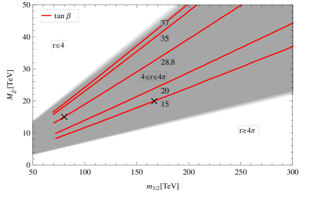
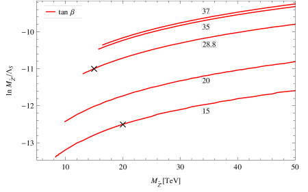
Figure 1: Constant $\tan{\beta}$ lines in the $M_{\tilde{Z}^{\prime}}-m_{3/2}$ plane (left) and the corresponding values of $\Lambda_{S}$ along such lines as a function of $M_{\tilde{Z}^{\prime}}$(right). The shaded region in the left plot corresponds to the allowed range in Eq. 7 ($r=m_{3/2}/M_{{\tilde{Z}}^{\prime}}$) for $c=1$. The position of our two illustration points is indicated by the crosses.

We choose two illustration points. The first has

$$m_{3/2}=80\,{\rm TeV},\quad M_{\tilde{Z}^{\prime}}=15\,{\rm TeV},\quad\Lambda_{S}\sim 10^{9}\,{\rm GeV}.$$ (17)

The top, bottom, and tau Yukawa couplings are taken to be

$$y_{t}=1,\,y_{b}=0.5,\,y_{\tau}=0.294$$ (18)

at the EW scale. For the first illustration point the vacuum parameters are

$$\tan\beta=28.8,\quad\langle S\rangle=11.9\,{\rm TeV}.$$ (19)

In Fig. 2 we show the running of the scalar soft masses of $H_{u}$, $H_{d}$ and $S$, for this point.

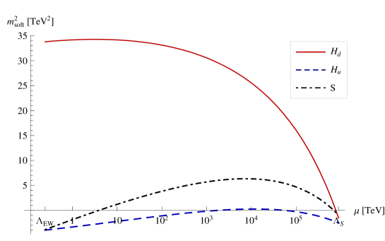
Figure 2: Scalar soft masses squared for the Higgs fields in the first illustration point.

The second illustration point has

$$m_{3/2}\approx 167\,{\rm TeV},\quad M_{\tilde{Z}^{\prime}}=20\,{\rm TeV},\quad\Lambda_{S}\sim 5\cdot 10^{9}\,{\rm GeV}.$$ (20)

The top, bottom, and tau Yukawa couplings are taken to be

$$y_{t}=1,\,y_{b}=0.257,\,y_{\tau}=0.154$$ (21)

at the EW scale. The vacuum parameters are

$$\tan\beta=15,\quad\langle S\rangle=25.2\,{\rm TeV}.$$ (22)

In the Tables 2 to 9 we display the details of the spectrum for both points. We use white and gray background colors to distinguish between the first and second points, respectively.

Due to the large $\tan\beta$ and the large vev of $S$, the vevs are strongly ordered : $\langle H_{d}^{0}\rangle\ll\langle H_{u}^{0}\rangle\ll\langle S\rangle$. As a result there is very little mixing in the extended Higgs sector ($H_{u}$,$H_{d}$,$S$). The Higgs masses, including the one-loop radiative corrections, and their composition are listed in Table 2.

	$m$ [TeV]		Composition[$\%$]
			$H_{d}$		$H_{u}$		$S$
$h^{0}$	0.138	0.142	0.1	0.4	99.9	99.6	0	0
$H^{0}_{1}$	2.79	5.69	0	0	0	0	100	100
$A^{0}$	4.78	6.85	99.9	99.6	0.1	0.4	0	0
$H^{0}_{2}$	4.78	6.85	99.9	99.6	0.1	0.4	0	0
$H^{\pm}$	4.78	6.85	99.9	99.6	0.1	0.4	-	-

Table 2: Neutral and charged Higgs masses (including radiative corrections) and composition, for point 1 (white background) and point 2 (gray background).

The radiative corrections can be quite substantial. For example, at tree level we have $m_{h^{0}}=85$ GeV, $m_{H^{0}_{1}}=2.78$ TeV, and $m_{H^{0}_{2}}=5.37$ TeV for the first illustration point. For the lightest Higgs boson, two-loop effects typically reduce the one-loop mass by a few GeV [35]. The radiative corrections to the charged Higgs masses were determined by $SU(2)_{L}$ symmetry and not by a direct calculation.

The gluino mass is shown in Table 3. We also include in the table the bino and wino mass parameters to compare with the standard anomaly mediation scenario. As described in the previous section, we find that like the standard AMSB the wino is the lightest of the gauginos, but unlike standard AMSB the gluino is lighter than the bino.

$M_{1}$ [TeV]		$M_{2}$ [TeV]		$M_{3}$ [TeV]
1.17	2.41	0.279	0.582	0.399	0.813

Table 3: Gaugino mass parameters for point 1 (white background) and point 2 (gray background). The neutralino and chargino mass eigenvalues are given in Tables 4 and 5, respectively.

As can be seen from Fig. 1, one can raise the overall scale and still find acceptable spectrum. One can vary the mass splitting between $M_{3}$ and $M_{2}$, which is approximately the mass difference between the gluino and the lightest supersymmetric particle (LSP), by increasing the overall scale. In Fig. 3 we show how such splitting as well as the gluino mass grow as we lift the $Z^{\prime}$-gaugino and gravitino masses along each constant $\tan{\beta}$ line in Fig. 1. Whether this mass splitting is less than $m_{t}$, bigger than $m_{t}$, or bigger than $2m_{t}$, has important implications to phenomenology, as discussed in detail in section 5. The largest splitting for our illustration points is for the second one, with $M_{3}-M_{2}\sim 230\ {\rm GeV}$, and we observe that for gluinos below a TeV we can achieve values up to the order of 300 GeV. The gluino masses we consider are not excluded by the jets $+\not{\!\!E}_{T}$ search at the Tevatron [36]. It is also possible to probe this scenario at the Tevatron if the gluino mass is in the range of 300 - 400 GeV.

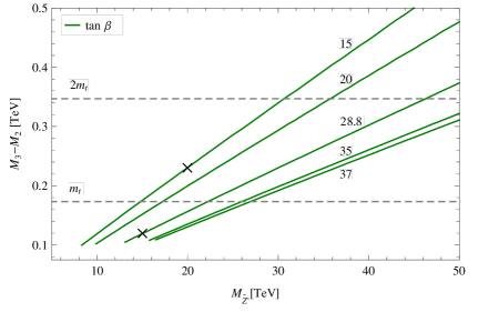
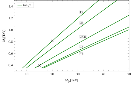
Figure 3: (Left) Mass splitting between the gluino and wino masses for each $\tan{\beta}$ line in Fig. 1. (Right) Gluino mass along the same lines. Again, the two points discussed in the text are indicated by a cross.

Similarly to the Higgs sector, there is generally very little mixing in the neutralino sector. The only exception are the Higgsinos, which mix within themselves almost maximally, due to the large effective $\mu$ term. The neutralino masses and composition are listed in Table 4. In our case, as can be seen especially in the first point, there is also some Higgsino-bino mixing because of the small difference between the effective $\mu$ ($=\lambda\langle S\rangle$) and $M_{1}$.

	$m_{\tilde{N}}$ [TeV]		Composition[$\%$]
			${\tilde{B}}$		${\tilde{W}}^{0}$		${\tilde{Z}^{\prime}}$		${\tilde{H}}_{d}^{0}$		${\tilde{H}}_{u}^{0}$		${\tilde{S}}$
${\tilde{N}}_{1}$	0.278	0.582	0	0	99.5	99.9	0	0	0.5	0.1	0	0	0	0
${\tilde{N}}_{2}$	0.612	1.81	0	0	0	0	4.6	9.2	0	0	0.1	0	95.3	90.7
${\tilde{N}}_{3}$	1.15	2.41	71.2	94.1	0.1	0	0	0	14.9	3.1	13.7	2.8	0	0
${\tilde{N}}_{4}$	1.19	2.52	0	0	0.2	0	0	0	49.8	50	50	50	0	0
${\tilde{N}}_{5}$	1.21	2.53	28.8	5.9	0.2	0.1	0	0	34.8	46.8	36.2	47.2	0	0
${\tilde{N}}_{6}$	12.7	17.8	0	0	0	0	95.4	90.8	0	0	0	0	4.6	9.2

Table 4: Neutralino masses and composition for point 1 (white background) and point 2 (gray background).

	$m_{\tilde{C}}$ [TeV]		Composition[$\%$]
			${\tilde{W}}^{\pm}$		${\tilde{H}}^{\pm}$
${\tilde{C}}_{1}$	0.278	0.581	99	99.8	1	0.2
${\tilde{C}}_{2}$	1.2	2.52	1	0.2	99	99.8

Table 5: Chargino masses and composition for point 1 (white background) and point 2 (gray background).

Due to the large difference between $M_{2}$ and the effective $\mu$ , the mixing in the chargino sector is also very small. The chargino spectrum is displayed in Table 5. The ${\tilde{C}}_{1}$ is expected to be heavier than the ${\tilde{N}}_{1}$ by $\sim 160$ MeV due to radiative corrections [37].

$1^{\mathrm{st}}$ and $2^{\mathrm{nd}}$ families						$3^{\mathrm{rd}}$ family
	$m_{\tilde{f}}$ [TeV]			$m_{\tilde{f}}$ [TeV]			$m_{\tilde{f}}$ [TeV]			$m_{\tilde{f}}$ [TeV]
${\tilde{u}}_{L},{\tilde{c}}_{L}$	2.42	3.75	${\tilde{u}}_{R},{\tilde{c}}_{R}$	4.11	4.72	${\tilde{t}}_{1}$	0.695	1.29	${\tilde{t}}_{2}$	3.16	1.81
${\tilde{d}}_{L},{\tilde{s}}_{L}$	2.42	3.75	${\tilde{d}}_{R},{\tilde{s}}_{R}$	4.7	7.22	${\tilde{b}}_{1}\approx{\tilde{b}}_{L}$	0.689	1.61	${\tilde{b}}_{2}\approx{\tilde{b}}_{R}$	4.28	7
${\tilde{\nu}^{e}}_{L},{\tilde{\nu}^{\mu}}_{L}$	4.65	5.74	${\tilde{\nu}^{e}}_{R},{\tilde{\nu}^{\mu}}_{R}$	3.05	4.95	${\tilde{\nu}^{\tau}}_{L}$	4.38	5.6	${\tilde{\nu}^{\tau}}_{R}$	3.05	4.95
${\tilde{e}}_{L},{\tilde{\mu}}_{L}$	4.65	5.74	${\tilde{e}}_{R},{\tilde{\mu}}_{R}$	12.2	18.1	${\tilde{\tau}}_{1}\approx{\tilde{\tau}}_{L}$	4.38	5.6	${\tilde{\tau}}_{2}\approx{\tilde{\tau}}_{R}$	12	18

Table 6: Sfermion masses for point 1 (white background) and point 2 (gray background). The mass mixing for third family sfermions is small except for the stops in the second point where the two diagonal entries in Eq. 11 are similar resulting in a large mixing. The values for the first (second) illustration point are $\sin\theta_{{\tilde{t}}_{L}{\tilde{t}}_{R}}=0.04(0.65)$, $\sin\theta_{{\tilde{b}}_{L}{\tilde{b}}_{R}}=0.007(0.003)$ and $\sin\theta_{{\tilde{\tau}}_{L}{\tilde{\tau}}_{R}}=0.0006(0.0003)$.

The MSSM sfermions are in the range of a few TeV. They range from the lightest, which is the lighter sbottom (stop) for the first (second) point, to the heaviest, which is the right-handed slepton. Their masses are given in Table 6. The MSSM sfermion masses are determined by the contributions from anomaly mediation, $Z^{\prime}$-gaugino mediation, and D-term contributions after $U(1)^{\prime}$ gauge symmetry breaking. Therefore, most features of the spectrum can be understood from the prediction of pure anomaly mediation and the choices of charges in Table 1. The anomaly contribution to the soft masses is negative not only for the first and second families of sleptons but for all the MSSM sfermions. This is because of the vanishing of the strong coupling $\beta$-function at one loop and the extra negative contribution from the $\beta$-function of the $Z^{\prime}$ gauge coupling. The $Z^{\prime}$-gaugino mediation leads to large positive contributions proportional to $Q_{i}^{2}$, raising the soft masses from the tachyonic region, as can be seen in Fig. 4. This dependence on the charge explains the difference between the first two generations of left-handed and right-handed squarks. The third generation squarks are generically lighter due to the effect of the Yukawa couplings in the running, which can in some cases turn some of the soft masses tachyonic again. From Fig. 4 (right) we observe that this is the case for the left-handed stop and sbottom in our particular example. The $D$-term contributions can be either positive or negative depending on $Q_{i}Q_{S}$. Although in general smaller, here they are responsible for returning the squared masses for the left-handed squarks back to the positive region.

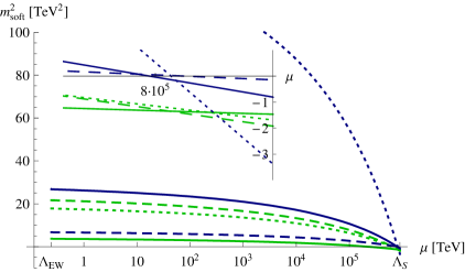
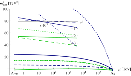
Figure 4: Running of the MSSM sfermion soft masses squared in the first illustration point. First and second families (left). Third family (right). A close view of the region near $\Lambda_{S}$ is displayed to illustrate the pure anomaly mediation contribution.

Similarly, the exotic sfermions range from the lightest, $\tilde{D}_{1}$, to the heaviest, $\tilde{E}_{2}$, which is also the heaviest sfermion in the spectrum. Their masses and mixings are given in Table 7. The exotic fermion masses are given in Table 8.

	$m_{\tilde{f}}$ [TeV]			$m_{\tilde{f}}$ [TeV]		$\sin\theta_{{\tilde{f}}{\tilde{f}}^{c}}$
${\tilde{D}}_{1}$	2.53	3.24	${\tilde{D}}_{2}$	6.41	11.6	0.48	0.63
${\tilde{E}}_{1}$	9.25	15.6	${\tilde{E}}_{2}$	12.8	20.6	0.37	0.55

Table 7: Exotic sfermion masses and mixings for point 1 (white background) and point 2 (gray background).

	$m_{f}$ [TeV]
$D$	3.57	7.56
$E$	5.95	12.6

Table 8: Exotic fermion masses for point 1 (white background) and point 2 (gray background).

Finally, the $Z^{\prime}$ gauge boson mass and $Z-Z^{\prime}$ mixing angle are listed in Table 9. The spectra are summarized in Figs. 5 and 6.

$M_{Z^{\prime}}$ [TeV]		$\sin\theta_{ZZ^{\prime}}$
2.78	5.68	3$\cdot$10-4	7$\cdot$10-5

Table 9: $Z^{\prime}$ mass and mixing for point 1 (white background) and point 2 (gray background).

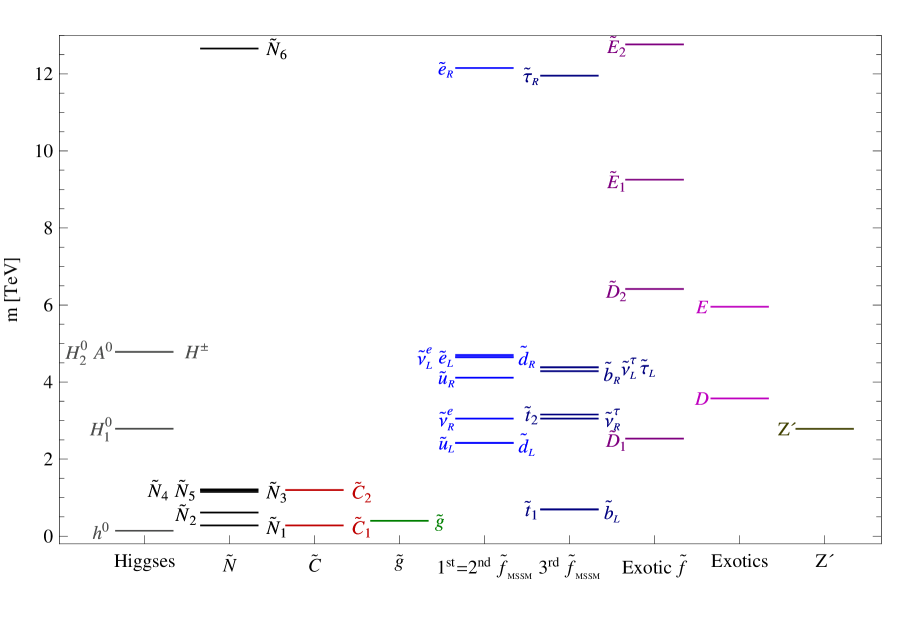
Figure 5: Spectrum of the first illustration point discussed in the text.

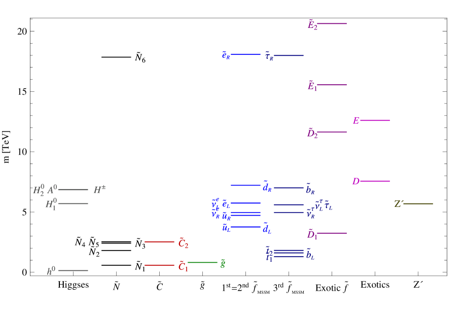
Figure 6: Spectrum of the second illustration point discussed in the text.

The fact that $m_{H_{1}}$ and $M_{Z^{\prime}}$ are approximately the same is not an accident. It arises from the fact that there is very little mixing in the Higgs sector. Consequently $H_{1}$ is almost “pure” $S$. If we now consider only the $S$ and $Z^{\prime}$ sector and allow for negative $m_{S}^{2}$, we can think of $m_{S}^{2}$ as arising from a Fayet-Iliopoulos term [38]. Adding a constant term to the scalar potential for $S$, we can write it as,

$$V=m^{2}_{S}|S|^{2}+\frac{g_{{{\mbox{\tiny$Z^{\prime}$}}}}^{2}}{2}Q_{S}^{2}|S|^{4}+\mbox{constant}=\frac{1}{2}\left(\xi-g_{{{\mbox{\tiny$Z^{\prime}$}}}}Q_{S}|S|^{2}\right)^{2},$$ (23)

where $\xi=-m_{S}^{2}/g_{{{\mbox{\tiny$Z^{\prime}$}}}}Q_{S}$. The vacuum in this case breaks the $U(1)^{\prime}$ gauge symmetry but not supersymmetry. The chiral and the vector multiplet are combined to form a massive vector multiplet with mass $\sqrt{2}|m_{S}|$.

Introducing a gaugino mass term breaks supersymmetry explicitly, but at tree level its presence only shifts the singlino and the $Z^{\prime}$ gaugino mass, while the scalar and vector components of the supermultiplet remain degenerate. This degeneracy will be lifted by other interactions of the scalar component of $S$, and its mixing, but these are still smaller effects, so to a good approximation $m_{H_{1}}$ and $M_{Z^{\prime}}$ are equal.

5 Conclusions

In this paper, we argued that combining $Z^{\prime}$ mediation with anomaly mediation is both a plausible and a feasible scenario. As an example , we have considered a particular realization and argued that its contribution can be naturally comparable to anomaly mediation. Such an approach solves the tachyonic slepton mass problem of anomaly mediation, and the need for fine-tuning in the original $Z^{\prime}$ mediation models. In this context, it is natural to consider an NMSSM-like model in which $U(1)^{\prime}$ gauge symmetry forbids a $\mu$ term in the superpotential. In this case, the $U(1)^{\prime}$ gauge symmetry breaking, the effective $\mu$ and $B_{\mu}$ terms, and the electroweak symmetry breaking must all be generated dynamically from UV input values. We found that it is not difficult to find viable models in this scenario. We presented two explicit examples with different low energy spectrum.

We comment on generic phenomenological features of this class of models. The gaugino spectrum is completely determined by the anomaly mediation. However, since we have to introduce additional exotic matter, the anomaly mediation contribution can be dramatically different from the MSSM prediction. Such a change can lead to significantly different phenomenology. In the specific class of models we considered here, the gluino only receives a contribution from 2-loop anomaly mediation, and is only somewhat heavier than the LSP (wino in this case). Such light gluinos can be copiously produced at the LHC. Since stops and sbottoms are typically lighter than the first two families of squarks, the decay products of the gluino are mainly dominated by the third generation states: $b\bar{b}+\tilde{N}_{0}$, $t+\bar{b}+\tilde{C}^{+}$, and $t\bar{t}+\tilde{N}_{0}$. However, the availability of decay channels involving top quarks depends on $M_{3}-M_{2}$. For the first illustration point $M_{3}-M_{2}<m_{t}$ and only the $b\bar{b}+\tilde{N}_{0}$ decay mode is possible. For the second illustration point $m_{t}<M_{3}-M_{2}<2m_{t}$ and both $b\bar{b}+\tilde{N}_{0}$ and $t+\bar{b}+\tilde{C}^{+}$ are possible. Requiring the gluino is lighter than a TeV, the largest value of $M_{3}-M_{2}$ is of the order of $300$ GeV. Different choices of the input charges may help in getting an even larger splitting. While the $b\bar{b}b\bar{b}+\not{\!\!E}_{T}$ signal is a very useful discovery channel, the decay channels which lead to multiple top final states have spectacular signals and can lead to early discovery at the LHC [39]. Another prominent feature of this scenario is the presence of a $Z^{\prime}$ gauge boson with $M_{Z^{\prime}}$ around several TeV, unlike the pure $Z^{\prime}$-gaugino mediation where $M_{Z^{\prime}}$ is typically very heavy. Such a $Z^{\prime}$ has an excellent chance of being discovered at the LHC. Detailed measurements of its properties, in particular its couplings to various Standard Model matter fields, especially leptons and third generation quarks, provide clues crucial to piecing together the complete picture of mediation of supersymmetry breaking. Such a $Z^{\prime}$ will also decay into superpartners, which also offers a good opportunity of studying their properties [40, 41]. In particular, in this model, $Z^{\prime}$ decay probably offers the only possibility of discovering and study the properties of the singlino.

Acknowledgments: We would like to thank Zohar Komargodski, Yael Shadmi and Jay Wacker for useful discussions. J.B. also gratefully acknowledges the hospitality of the Institute for Advanced Study at Princeton during part of this work. The work of J.B. is supported by MICINN project FPA2006-05294 and Junta de Andalucía projects FQM 101, FQM 437 and FQM 03048. The work of P.L. is supported by the IBM Einstein Fellowship and by NSF grant PHY-0503584. The work of G.P. is supported in part by the Department of Energy grants DE-FG02-90ER40542 and DE-FG02-90ER40560, and by the United States-Israel Bi-national Science Foundation grant 2006280. The work of L.-T. W. is supported by the National Science Foundation under grant PHY-0756966 and the Department of Energy under grant DE-FG02-90ER40542.

Appendix A $U(1)^{\prime}$ charges

We normalize all the $U(1)^{\prime}$ charges such that $Q_{H_{d}}=1$. Defining $Q_{H_{u}}=x$ and $Q_{Q}=y$, the other charges are

$$Q_{u^{c}}=-x-y,\quad Q_{d^{c}}=-1-y,\quad Q_{L}=-\frac{1}{3}(1+x)-3y,$$

$$Q_{e^{c}}=-1+\frac{1+x}{3}+3y,\quad Q_{\nu^{c}}=-x+\frac{1+x}{3}+3y$$

$$Q_{S}=-1-x,\quad Q_{D}=\frac{2}{9}(3+x-3y)+\sqrt{2(1+3y)(1-x+6y)},\quad Q_{D^{c}}=-Q_{S}-Q_{D}$$

$$Q_{E}=-3y-\frac{3}{2}Q_{D}+2,\quad Q_{E^{c}}=-Q_{S}-Q_{E}.$$ (24)

Appendix B Boundary conditions

We assume that at a scale $\Lambda_{S}$ the gaugino and scalar masses are generated from the anomaly contribution. We use the general expressions from [25],

$$M_{\lambda} = -\frac{g^{2}}{2}\frac{dg^{-2}}{d\ln\mu}m_{3/2}=\frac{\beta_{g}}{g}m_{3/2}$$

$$m_{\tilde{Q}}^{2} = -\frac{1}{4}\frac{d^{2}\ln Z_{Q}}{d(\ln\mu)^{2}}m_{3/2}^{2}=-\frac{1}{4}\left(\frac{\partial\gamma}{\partial g}\beta_{g}+\frac{\partial\gamma}{\partial y}\beta_{y}\right)m_{3/2}^{2}$$

$$A_{y} = \frac{1}{2}\sum_{i}\frac{d\ln Z_{Q_{i}}}{d\ln\mu}m_{3/2}=-{\beta_{y}}m_{3/2},$$ (25)

where $\gamma\equiv{d\ln Z}/{d\ln\mu}$, $\beta_{g}\equiv{dg}/{d\ln\mu}$, $\beta_{y}\equiv{dy}/{d\ln\mu}$, and $A_{y}$ is defined as in ${\cal L}=-A_{y}~{}\phi_{1}\,\phi_{2}\,\phi_{3}$ +h.c.. At one loop

$$\gamma^{i}_{j}=-\frac{1}{16\pi^{2}}\left[y^{imn}y^{*}_{jmn}-4g_{a}^{2}C_{a}(i)\delta^{i}_{j}\right].$$ (26)

To determine the boundary conditions, we need the beta functions for the gauge and Yukawa couplings. In the mixed scenario the dominant contribution to the gaugino masses (apart from the $Z^{\prime}$ gaugino) is the anomaly contribution. For the models of [5, 6], the beta function for $g_{3}$ vanishes at one loop. As a result at one loop the gluino is massless. It will get a non-zero contribution at two-loop order. For consistency we will use the two-loop expressions for all three gauge coupling beta functions. To derive the beta functions we use the general expressions in [42, 43, 44, 45]. In the following $n_{D}=3$ and $n_{E}=2$.

B.1 Gauge and Yukawa $\beta$ functions

The gauge coupling $\beta$ functions are

$$\beta_{g_{1}} = \frac{g_{1}^{3}}{16\pi^{2}}\bigg{\{}\frac{51}{5}+\frac{1}{16\pi^{2}}\bigg{[}24g_{3}^{2}+\frac{27}{5}g_{2}^{2}+\frac{351}{25}g_{1}^{2}+g_{z^{\prime}}^{2}\frac{12}{5}{\rm Tr}\left(Y^{2}Q^{2}\right)$$

$$\qquad\quad-\frac{26}{5}y_{t}^{2}-\frac{14}{5}y_{b}^{2}-\frac{18}{5}y_{\tau}^{2}-\frac{6}{5}\lambda^{2}-\frac{12}{5}y_{D}^{2}-\frac{24}{5}y_{E}^{2}\bigg{]}\bigg{\}}$$

$$\beta_{g_{2}} = \frac{g_{2}^{3}}{16\pi^{2}}\bigg{\{}1+\frac{1}{16\pi^{2}}\bigg{[}24g_{3}^{2}+25g_{2}^{2}+\frac{9}{5}g_{1}^{2}+2g_{z^{\prime}}^{2}(Q_{H_{d}}^{2}+Q^{2}_{H_{u}}+3(Q_{L}^{2}+3Q_{Q}^{2}))$$

$$\qquad\quad-6y_{t}^{2}-6y_{d}^{2}-2y_{\tau}^{2}-2\lambda^{2}\bigg{]}\bigg{\}}$$

$$\beta_{g_{3}} = \frac{g_{3}^{3}}{(16\pi^{2})^{2}}\bigg{[}48g_{3}^{2}+9g_{2}^{2}+3g_{1}^{2}+6g_{z^{\prime}}^{2}(Q_{D}^{2}+Q_{D^{c}}^{2}+2Q_{Q}^{2}+Q_{u^{c}}^{2}+Q_{d^{c}}^{2})-4y_{t}^{2}-4y_{b}^{2}-6y_{D}^{2}\bigg{]}$$

$$\beta_{g_{{{\mbox{\tiny$Z^{\prime}$}}}}} = \frac{g_{{{\mbox{\tiny$Z^{\prime}$}}}}^{3}}{16\pi^{2}}\bigg{\{}{\rm Tr}\left(Q^{2}\right)+\frac{1}{16\pi^{2}}\bigg{[}4g_{{{\mbox{\tiny$Z^{\prime}$}}}}^{2}{\rm Tr}\left(Q^{4}\right)+g_{1}^{2}\frac{12}{5}{\rm Tr}\left(Y^{2}Q^{2}\right)$$

$$\qquad\quad+6g_{2}^{2}(Q_{H_{d}}^{2}+Q^{2}_{H_{u}}+3(Q_{L}^{2}+3Q_{Q}^{2}))+48g_{3}^{2}(Q_{D}^{2}+Q_{D^{c}}^{2}+2Q_{Q}^{2}+Q_{u^{c}}^{2}+Q_{d^{c}}^{2})-$$

$$\qquad\quad-12(Q_{u^{c}}^{2}+Q_{Q}^{2}+Q_{H_{u}}^{2})y_{t}^{2}-12(Q_{d^{c}}^{2}+Q_{Q}^{2}+Q_{H_{d}}^{2})y_{b}^{2}-4(Q_{e^{c}}^{2}+Q_{L}^{2}+Q_{H_{d}}^{2})y_{e}^{2}$$

$$\qquad\quad-18(Q_{D^{c}}^{2}+Q_{D}^{2}+Q_{S}^{2})y_{D}^{2}-4(Q_{E^{c}}^{2}+Q_{E}^{2}+Q_{S}^{2})y_{E}^{2}-4(Q_{H_{u}}^{2}+Q_{H_{d}}^{2}+Q_{S}^{2})\lambda^{2}\bigg{]}\bigg{\}}.$$

The relevant $\beta$ functions for the Yukawa couplings are

$$\beta_{y_{t}} = \frac{y_{t}}{16\pi^{2}}\bigg{[}\lambda^{2}+6y_{t}^{2}+y_{b}^{2}-\frac{16}{3}g_{3}^{2}-3g_{2}^{2}-\frac{13}{15}g_{1}^{2}-2g_{{{\mbox{\tiny$Z^{\prime}$}}}}^{2}(Q_{H_{u}}^{2}+Q_{Q}^{2}+Q_{u^{c}}^{2})\bigg{]}$$

$$\beta_{y_{b}} = \frac{y_{b}}{16\pi^{2}}\bigg{[}\lambda^{2}+6y_{b}^{2}+y_{t}^{2}+y_{e}^{2}-\frac{16}{3}g_{3}^{2}-3g_{2}^{2}-\frac{7}{15}g_{1}^{2}-2g_{{{\mbox{\tiny$Z^{\prime}$}}}}^{2}(Q_{H_{d}}^{2}+Q_{Q}^{2}+Q_{d^{c}}^{2})\bigg{]}$$

$$\beta_{y_{\tau}} = \frac{y_{\tau}}{16\pi^{2}}\bigg{[}\lambda^{2}+3y_{b}^{2}+4y_{\tau}^{2}-3g_{2}^{2}-\frac{9}{5}g_{1}^{2}-2g_{{{\mbox{\tiny$Z^{\prime}$}}}}^{2}(Q_{H_{d}}^{2}+Q_{L}^{2}+Q_{e^{c}}^{2})\bigg{]}$$

$$\beta_{\lambda} = \frac{\lambda}{16\pi^{2}}\bigg{[}4\lambda^{2}+3y_{t}^{2}+3y_{b}^{2}+y_{\tau}^{2}+3n_{D}\,y_{D}^{2}+n_{E}\,y_{E}^{2}-3g_{2}^{2}-\frac{3}{5}g_{1}^{2}-2g^{2}_{z^{\prime}}\left(Q_{S}^{2}+Q_{H_{u}}^{2}+Q^{2}_{H_{d}}\right)\bigg{]}$$

$$\beta_{y_{D}} = \frac{y_{D}}{16\pi^{2}}\bigg{[}2\lambda^{2}+(3n_{D}+2)y_{D}^{2}+n_{E}y_{E}^{2}-\frac{16}{3}g_{3}^{2}-\frac{6}{5}g_{1}^{2}(Y_{D}^{2}+Y_{D^{c}}^{2})-2g_{{{\mbox{\tiny$Z^{\prime}$}}}}^{2}(Q_{S}^{2}+Q_{D}^{2}+Q_{D^{c}}^{2})\bigg{]}$$

$$\beta_{y_{E}} = \frac{y_{E}}{16\pi^{2}}\bigg{[}2\lambda^{2}+3n_{D}y_{D}^{2}+(n_{E}+2)y_{E}^{2}-\frac{6}{5}g_{1}^{2}(Y_{E}^{2}+Y_{E^{c}}^{2})-2g_{{{\mbox{\tiny$Z^{\prime}$}}}}^{2}(Q_{S}^{2}+Q_{E}^{2}+Q_{E^{c}}^{2})\bigg{]}.$$

We have set all the SM Yukawas, apart from $y_{t},\,y_{b}$, and $y_{\tau}$, to zero.

B.2 Gaugino masses

The MSSM gaugino masses are

$$M_{3}(\Lambda_{S})=\frac{\beta_{g_{3}}}{g_{3}}\,m_{3/2},\quad M_{2}(\Lambda_{S})=\frac{\beta_{g_{2}}}{g_{2}}\,m_{3/2},\quad M_{1}(\Lambda_{S})=\frac{\beta_{g_{1}}}{g_{1}}\,m_{3/2}.$$ (29)

The $Z^{\prime}$ gaugino mass, $M_{\tilde{Z}^{\prime}}$, is a free parameter. If we fix it at the scale $M_{\tilde{Z}^{\prime}}$, its value at $\Lambda_{S}$ would be

$$M_{\tilde{Z}^{\prime}}(\Lambda_{S})=M_{\tilde{Z}^{\prime}}(M_{\tilde{Z}^{\prime}})\left[1-\frac{{\rm Tr}\left(Q^{2}\right)g_{{{\mbox{\tiny$Z^{\prime}$}}}}^{2}(\Lambda_{s})}{8\pi^{2}}\ln\left(\frac{\Lambda_{S}}{M_{\tilde{Z}^{\prime}}}\right)\right].$$ (30)

B.3 Scalar masses

The general expression for the scalar masses is schematically

$$m^{2}=\frac{m_{3/2}^{2}}{16\pi^{2}}\left[\#\,y\,\beta_{y}-\sum_{i}\,2\,C_{i}\,g_{i}\,\beta_{i}\right],$$ (31)

where $\#$ is an integer which depends on the specific form of the Yukawa coupling. The constants $C_{i}$ are

$$C_{3}=4/3,\quad C_{2}=3/4,\quad C_{1}=3\,Y^{2}/5,\quad C_{z^{\prime}}=Q^{2},$$ (32)

where $Y$ is the hypercharge and $Q$ is the $U(1)^{\prime}$ charge.

The expression for the soft masses at the SUSY breaking scale are, for $S,H_{u},$ and $H_{d}$,

$$m^{2}_{S} = \frac{m^{2}_{3/2}}{16\pi^{2}}\left(2\lambda\,\beta_{\lambda}+3n_{D}y_{D}\,\beta_{y_{D}}+n_{E}y_{E}\,\beta_{y_{E}}-2g_{{{\mbox{\tiny$Z^{\prime}$}}}}Q_{S}^{2}\,\beta_{g_{{{\mbox{\tiny$Z^{\prime}$}}}}}\right)$$

$$m^{2}_{H_{u}} = \frac{m^{2}_{3/2}}{16\pi^{2}}\left(\lambda\,\beta_{\lambda}+3y_{t}\,\beta_{y_{t}}-\frac{6}{4}g_{2}\,\beta_{g_{2}}-\frac{6}{5}Y^{2}_{H_{u}}g_{1}\,\beta_{g_{1}}-2g_{{{\mbox{\tiny$Z^{\prime}$}}}}Q_{H_{u}}^{2}\,\beta_{g_{{{\mbox{\tiny$Z^{\prime}$}}}}}\right)$$

$$m^{2}_{H_{d}} = \frac{m^{2}_{3/2}}{16\pi^{2}}\left(\lambda\,\beta_{\lambda}+3y_{b}\,\beta_{y_{b}}+y_{\tau}\,\beta_{y_{\tau}}-\frac{6}{4}g_{2}\,\beta_{g_{2}}-\frac{6}{5}Y^{2}_{H_{d}}g_{1}\,\beta_{g_{1}}-2g_{{{\mbox{\tiny$Z^{\prime}$}}}}Q_{H_{d}}^{2}\,\beta_{g_{{{\mbox{\tiny$Z^{\prime}$}}}}}\right);$$ (33)

for the scalar exotics,

$$m^{2}_{\tilde{D}} = \frac{m^{2}_{3/2}}{16\pi^{2}}\left(y_{D}\,\beta_{y_{D}}-\frac{8}{3}g_{3}\,\beta_{g_{3}}-\frac{6}{5}Y^{2}_{D}g_{1}\,\beta_{g_{1}}-2g_{{{\mbox{\tiny$Z^{\prime}$}}}}Q_{D}^{2}\,\beta_{g_{{{\mbox{\tiny$Z^{\prime}$}}}}}\right)$$

$$m^{2}_{\tilde{D}^{c}} = \frac{m^{2}_{3/2}}{16\pi^{2}}\left(y_{D}\,\beta_{y_{D}}-\frac{8}{3}g_{3}\,\beta_{g_{3}}-\frac{6}{5}Y^{2}_{D^{c}}g_{1}\,\beta_{g_{1}}-2g_{{{\mbox{\tiny$Z^{\prime}$}}}}Q_{D^{c}}^{2}\,\beta_{g_{{{\mbox{\tiny$Z^{\prime}$}}}}}\right)$$

$$m^{2}_{\tilde{E}} = \frac{m^{2}_{3/2}}{16\pi^{2}}\left(y_{E}\,\beta_{y_{E}}-\frac{6}{5}Y^{2}_{E}g_{1}\,\beta_{g_{1}}-2g_{{{\mbox{\tiny$Z^{\prime}$}}}}Q_{E}^{2}\,\beta_{g_{{{\mbox{\tiny$Z^{\prime}$}}}}}\right)$$

$$m^{2}_{\tilde{E}^{c}} = \frac{m^{2}_{3/2}}{16\pi^{2}}\left(y_{E}\,\beta_{y_{E}}-\frac{6}{5}Y^{2}_{E^{c}}g_{1}\,\beta_{g_{1}}-2g_{{{\mbox{\tiny$Z^{\prime}$}}}}Q_{E^{c}}^{2}\,\beta_{g_{{{\mbox{\tiny$Z^{\prime}$}}}}}\right);$$ (34)

for the third generation squarks

$$m^{2}_{\tilde{Q}_{3}} = \frac{m^{2}_{3/2}}{16\pi^{2}}\left(y_{t}\,\beta_{y_{t}}+y_{b}\,\beta_{y_{b}}-\frac{8}{3}g_{3}\,\beta_{g_{3}}-\frac{6}{4}g_{2}\,\beta_{g_{2}}-\frac{6}{5}Y^{2}_{Q}g_{1}\,\beta_{g_{1}}-2g_{{{\mbox{\tiny$Z^{\prime}$}}}}Q_{Q}^{2}\,\beta_{g_{{{\mbox{\tiny$Z^{\prime}$}}}}}\right)$$

$$m^{2}_{\tilde{t}^{c}} = \frac{m^{2}_{3/2}}{16\pi^{2}}\left(2y_{t}\,\beta_{y_{t}}-\frac{8}{3}g_{3}\,\beta_{g_{3}}-\frac{6}{5}Y^{2}_{u^{c}}g_{1}\,\beta_{g_{1}}-2g_{{{\mbox{\tiny$Z^{\prime}$}}}}Q_{u^{c}}^{2}\,\beta_{g_{{{\mbox{\tiny$Z^{\prime}$}}}}}\right)$$

$$m^{2}_{\tilde{b}^{c}} = \frac{m^{2}_{3/2}}{16\pi^{2}}\left(2y_{b}\,\beta_{y_{b}}-\frac{8}{3}g_{3}\,\beta_{g_{3}}-\frac{6}{5}Y^{2}_{d^{c}}g_{1}\,\beta_{g_{1}}-2g_{{{\mbox{\tiny$Z^{\prime}$}}}}Q_{d^{c}}^{2}\,\beta_{g_{{{\mbox{\tiny$Z^{\prime}$}}}}}\right);$$ (35)

for the first two generations of squarks,

$$m^{2}_{\tilde{Q}_{i}} = \frac{m^{2}_{3/2}}{16\pi^{2}}\left(-\frac{8}{3}g_{3}\,\beta_{g_{3}}-\frac{6}{4}g_{2}\,\beta_{g_{2}}-\frac{6}{5}Y^{2}_{Q}g_{1}\,\beta_{g_{1}}-2g_{{{\mbox{\tiny$Z^{\prime}$}}}}Q_{Q}^{2}\,\beta_{g_{{{\mbox{\tiny$Z^{\prime}$}}}}}\right)$$

$$m^{2}_{\tilde{u}^{c}_{i}} = \frac{m^{2}_{3/2}}{16\pi^{2}}\left(-\frac{8}{3}g_{3}\,\beta_{g_{3}}-\frac{6}{5}Y^{2}_{u^{c}}g_{1}\,\beta_{g_{1}}-2g_{{{\mbox{\tiny$Z^{\prime}$}}}}Q_{u^{c}}^{2}\,\beta_{g_{{{\mbox{\tiny$Z^{\prime}$}}}}}\right)$$

$$m^{2}_{\tilde{d}^{c}_{i}} = \frac{m^{2}_{3/2}}{16\pi^{2}}\left(-\frac{8}{3}g_{3}\,\beta_{g_{3}}-\frac{6}{5}Y^{2}_{d^{c}}g_{1}\,\beta_{g_{1}}-2g_{{{\mbox{\tiny$Z^{\prime}$}}}}Q_{d^{c}}^{2}\,\beta_{g_{{{\mbox{\tiny$Z^{\prime}$}}}}}\right);$$ (36)

for the third generation of charged sleptons,

$$m^{2}_{\tilde{L}_{3}} = \frac{m^{2}_{3/2}}{16\pi^{2}}\left(y_{\tau}\,\beta_{y_{\tau}}-\frac{6}{4}g_{2}\,\beta_{g_{2}}-\frac{6}{5}Y^{2}_{L}g_{1}\,\beta_{g_{1}}-2g_{{{\mbox{\tiny$Z^{\prime}$}}}}Q_{L}^{2}\,\beta_{g_{{{\mbox{\tiny$Z^{\prime}$}}}}}\right)$$

$$m^{2}_{\tilde{\tau}^{c}} = \frac{m^{2}_{3/2}}{16\pi^{2}}\left(2y_{\tau}\,\beta_{y_{\tau}}-\frac{6}{5}Y^{2}_{e^{c}}g_{1}\,\beta_{g_{1}}-2g_{{{\mbox{\tiny$Z^{\prime}$}}}}Q_{e^{c}}^{2}\,\beta_{g_{{{\mbox{\tiny$Z^{\prime}$}}}}}\right);$$ (37)

and for the rest of the sleptons,

$$m^{2}_{\tilde{L}_{i}} = \frac{m^{2}_{3/2}}{16\pi^{2}}\left(-\frac{6}{4}g_{2}\,\beta_{g_{2}}-\frac{6}{5}Y^{2}_{L}g_{1}\,\beta_{g_{1}}-2g_{{{\mbox{\tiny$Z^{\prime}$}}}}Q_{L}^{2}\,\beta_{g_{{{\mbox{\tiny$Z^{\prime}$}}}}}\right)$$

$$m^{2}_{\tilde{e}^{c}_{i}} = \frac{m^{2}_{3/2}}{16\pi^{2}}\left(-\frac{6}{5}Y^{2}_{e^{c}}g_{1}\,\beta_{g_{1}}-2g_{{{\mbox{\tiny$Z^{\prime}$}}}}Q_{e^{c}}^{2}\,\beta_{g_{{{\mbox{\tiny$Z^{\prime}$}}}}}\right)$$

$$m^{2}_{\tilde{\nu}^{c}_{i}} = \frac{m^{2}_{3/2}}{16\pi^{2}}\left(-2g_{{{\mbox{\tiny$Z^{\prime}$}}}}Q_{\nu^{c}}^{2}\,\beta_{g_{{{\mbox{\tiny$Z^{\prime}$}}}}}\right).$$ (38)

B.4 $A$ terms

The non-zero Yukawa couplings are $y_{t},y_{b},y_{\tau},\,\lambda,\,y_{D}$ and $y_{E}$. The corresponding $A$ terms are:

$$A_{t}=-\beta_{y_{t}}m_{3/2},\quad A_{b}=-\beta_{y_{b}}m_{3/2},\quad A_{\tau}=-\beta_{y_{\tau}}m_{3/2},\quad$$

$$A_{\lambda}=-\beta_{\lambda}m_{3/2},\quad A_{D}=-\beta_{y_{D}}m_{3/2},\quad A_{E}=-\beta_{y_{E}}m_{3/2}.$$ (39)

Appendix C RGE equations

To derive the RGEs we use the general expressions in [42, 43, 44, 45].

C.1 Gauge and Yukawa couplings

The gauge coupling RGEs are

$$dg_{i}/d\ln\mu=\beta_{g_{i}},$$ (40)

where $i=1,2,3,Z^{\prime}$ and the $\beta_{i}$ are given in (B.1).

The Yukawa RGEs are

$$dy_{i}/d\ln\mu=\beta_{y_{i}},$$ (41)

where $i=t,b,\tau,\lambda,D,E$ and the $\beta_{i}$ are given in (B.1).

C.2 Gaugino masses

The RGEs for the gaugino masses are

$$\frac{dM_{1}}{d\ln\mu} = \frac{g_{1}^{2}}{16\pi^{2}}\Bigg{\{}\frac{102}{5}M_{1}+\frac{2}{16\pi^{2}}\bigg{[}24g_{3}^{2}(M_{1}+M_{3})+\frac{27}{5}g_{2}^{2}(M_{1}+M_{2})+\frac{351}{25}g_{1}^{2}(2M_{1})$$

$$+g_{z^{\prime}}^{2}\frac{12}{5}{\rm Tr}\left(Y^{2}Q^{2}\right)(M_{1}+M_{\tilde{Z}^{\prime}}))$$

$$+M_{1}\Big{(}-\frac{26}{5}y_{t}^{2}-\frac{14}{5}y_{b}^{2}-\frac{18}{5}y_{\tau}^{2}-\frac{6}{5}\lambda^{2}-\frac{12}{5}y_{D}^{2}-\frac{24}{5}y_{E}^{2}\Big{)}$$

$$+\frac{26}{5}A_{t}y_{t}+\frac{14}{5}A_{b}y_{b}+\frac{18}{5}A_{\tau}y_{\tau}+\frac{6}{5}A_{\lambda}\lambda+\frac{12}{5}A_{D}y_{D}+\frac{24}{5}A_{E}y_{E}\bigg{]}\Bigg{\}}$$

$$\frac{dM_{2}}{d\ln\mu} = \frac{g_{2}^{2}}{16\pi^{2}}\Bigg{\{}2M_{2}+\frac{2}{16\pi^{2}}\bigg{[}24g_{3}^{2}(M_{2}+M_{3})+25g_{2}^{2}(2M_{2})+\frac{9}{5}g_{1}^{2}(M_{2}+M_{1})$$

$$+2g_{z^{\prime}}^{2}(Q_{H_{d}}^{2}+Q^{2}_{H_{u}}+3(Q_{L}^{2}+3Q_{Q}^{2}))(M_{2}+M_{\tilde{Z}^{\prime}})$$

$$+M_{2}\Big{(}-6y_{t}^{2}-6y_{b}^{2}-2y_{\tau}^{2}-2\lambda^{2}\Big{)}+6A_{t}y_{t}+6A_{b}y_{b}+2A_{\tau}y_{\tau}+2A_{\lambda}\lambda\bigg{]}\Bigg{\}}$$

$$\frac{dM_{3}}{d\ln\mu} = \frac{2g_{3}^{2}}{(16\pi^{2})^{2}}\bigg{[}48g_{3}^{2}(2M_{3})+9g_{2}^{2}(M_{3}+M_{2})+3g_{1}^{2}(M_{3}+M_{1})+M_{3}\Big{(}-4y_{t}^{2}-4y_{b}^{2}-6y_{D}^{2}\Big{)}$$

$$+6g_{z^{\prime}}^{2}(Q_{D}^{2}+Q_{D^{c}}^{2}+2Q_{Q}^{2}+Q_{u^{c}}^{2}+Q_{d^{c}}^{2})(M_{3}+M_{\tilde{Z}^{\prime}})+4A_{t}y_{t}+4A_{b}y_{b}+6A_{D}y_{D}\bigg{]}$$

$$\frac{dM_{\tilde{Z}^{\prime}}}{d\ln\mu} = \frac{g_{{{\mbox{\tiny$Z^{\prime}$}}}}^{2}}{16\pi^{2}}\Bigg{\{}2{\rm Tr}\left(Q^{2}\right)M_{\tilde{Z}^{\prime}}+\frac{2}{16\pi^{2}}\bigg{[}4g_{{{\mbox{\tiny$Z^{\prime}$}}}}^{2}{\rm Tr}\left(Q^{4}\right)(2M_{\tilde{Z}^{\prime}})+g_{1}^{2}\frac{12}{5}{\rm Tr}\left(Y^{2}Q^{2}\right)(M_{\tilde{Z}^{\prime}}+M_{1})$$

$$+6g_{2}^{2}(Q_{H_{d}}^{2}+Q^{2}_{H_{u}}+3(Q_{L}^{2}+3Q_{Q}^{2}))(M_{\tilde{Z}^{\prime}}+M_{2})$$

$$+48g_{3}^{2}(Q_{D}^{2}+Q_{D^{c}}^{2}+2Q_{Q}^{2}+Q_{u^{c}}^{2}+Q_{d^{c}}^{2})(M_{\tilde{Z}^{\prime}}+M_{3})+$$

$$+12(Q_{u^{c}}^{2}+Q_{Q}^{2}+Q_{H_{u}}^{2})(A_{t}-M_{\tilde{Z}^{\prime}}y_{t})y_{t}+12(Q_{d^{c}}^{2}+Q_{Q}^{2}+Q_{H_{d}}^{2})(A_{b}-M_{\tilde{Z}^{\prime}}y_{b})y_{b}+$$

$$+4(Q_{H_{d}}^{2}+Q_{L}^{2}+Q_{e^{c}}^{2})(A_{\tau}-M_{\tilde{Z}^{\prime}}y_{\tau})+4(Q_{H_{u}}^{2}+Q_{H_{d}}^{2}+Q_{S}^{2})(A_{\lambda}-M_{\tilde{Z}^{\prime}}\lambda)+$$

$$+18(Q_{D^{c}}^{2}+Q_{D}^{2}+Q_{S}^{2})(A_{D}-M_{\tilde{Z}^{\prime}}y_{D})y_{D}+4(Q_{E^{c}}^{2}+Q_{E}^{2}+Q_{S}^{2})(A_{E}-M_{\tilde{Z}^{\prime}}y_{E})y_{E}\lambda\bigg{]}\Bigg{\}}.$$

C.3 Scalar masses

The RGEs for the soft masses are given below. The $U(1)_{Y}$ and $U(1)^{\prime}$ $D$-term contributions which are of the form Tr($Ym_{i}^{2}$) and Tr($Qm_{i}^{2}$) are not included. As explained in [6], at one-loop order the RGEs for these traces are homogeneous equations. Using the expressions of appendix B.3, one can show that these traces vanish at $\mu=\Lambda_{S}$. As a result they vanish for all scales and need not be included in the RGEs for the soft masses. We have also verified explicitly that numerically solving the soft masses RGEs with and without these traces give the same result.

The expression for RGEs of the soft masses, are for $S,H_{u},$ and $H_{d}$,

$$16\pi^{2}\,\frac{dm_{S}^{2}}{d\ln\mu} = -8g_{{{\mbox{\tiny$Z^{\prime}$}}}}^{2}Q_{S}^{2}M_{\tilde{Z}^{\prime}}^{2}+4\lambda^{2}(m_{S}^{2}+m_{H_{u}}^{2}+m_{H_{d}}^{2})$$

$$+6n_{D}y_{D}^{2}(m_{S}^{2}+m_{\tilde{D}}^{2}+m_{\tilde{D}^{c}}^{2})+2n_{E}y_{E}^{2}(m_{S}^{2}+m_{\tilde{E}}^{2}+m_{\tilde{E}^{c}}^{2})$$

$$+4A^{2}_{\lambda}+2n_{E}A_{E}^{2}+6n_{D}A_{D}^{2}$$

$$16\pi^{2}\,\frac{dm_{H_{u}}^{2}}{d\ln\mu} = -8g_{{{\mbox{\tiny$Z^{\prime}$}}}}^{2}Q_{H_{u}}^{2}M_{\tilde{Z}^{\prime}}^{2}-6M_{2}^{2}g_{2}^{2}-\frac{24}{5}M_{1}^{2}g_{1}^{2}Y_{H_{u}}^{2}$$

$$+2\lambda^{2}(m_{S}^{2}+m_{H_{u}}^{2}+m_{H_{d}}^{2})+6y_{t}^{2}(m_{H_{u}}^{2}+m_{\tilde{Q}_{3}}^{2}+m_{\tilde{t}^{c}}^{2})+6A_{t}^{2}+2A_{\lambda}^{2}$$

$$16\pi^{2}\,\frac{dm_{H_{d}}^{2}}{d\ln\mu} = -8g_{{{\mbox{\tiny$Z^{\prime}$}}}}^{2}Q_{H_{d}}^{2}M_{\tilde{Z}^{\prime}}^{2}-6M_{2}^{2}g_{2}^{2}-\frac{24}{5}M_{1}^{2}g_{1}^{2}Y_{H_{d}}^{2}$$ (43)

$$+2\lambda^{2}(m_{S}^{2}+m_{H_{u}}^{2}+m_{H_{d}}^{2})+6y_{b}^{2}(m_{H_{d}}^{2}+m_{\tilde{Q}_{3}}^{2}+m_{\tilde{b}^{c}}^{2})+2y_{\tau}^{2}(m_{H_{d}}^{2}+m_{\tilde{L}_{3}}^{2}+m_{\tilde{\tau}^{c}}^{2})$$

$$+6A_{b}^{2}+2A_{\tau}^{2}+2A_{\lambda}^{2};$$

for the scalar exotics,

$$16\pi^{2}\,\frac{dm_{\tilde{D}}^{2}}{d\ln\mu} = -8g_{{{\mbox{\tiny$Z^{\prime}$}}}}^{2}Q_{D}^{2}M_{\tilde{Z}^{\prime}}^{2}-\frac{32}{3}M_{3}^{2}g_{3}^{2}-\frac{24}{5}M_{1}^{2}g_{1}^{2}Y_{D}^{2}+2y_{D}^{2}(m_{S}^{2}+m_{\tilde{D}}^{2}+m_{\tilde{D}^{c}}^{2})+2A_{D}^{2}$$

$$16\pi^{2}\,\frac{dm_{\tilde{D}^{c}}^{2}}{d\ln\mu} = -8g_{{{\mbox{\tiny$Z^{\prime}$}}}}^{2}Q_{D^{c}}^{2}M_{\tilde{Z}^{\prime}}^{2}-\frac{32}{3}M_{3}^{2}g_{3}^{2}-\frac{24}{5}M_{1}^{2}g_{1}^{2}Y_{D^{c}}^{2}+2y_{D}^{2}(m_{S}^{2}+m_{\tilde{D}}^{2}+m_{\tilde{D}^{c}}^{2})+2A_{D}^{2}$$

$$16\pi^{2}\,\frac{dm_{\tilde{E}}^{2}}{d\ln\mu} = -8g_{{{\mbox{\tiny$Z^{\prime}$}}}}^{2}Q_{E}^{2}M_{\tilde{Z}^{\prime}}^{2}-\frac{24}{5}M_{1}^{2}g_{1}^{2}Y_{E}^{2}+2y_{E}^{2}(m_{S}^{2}+m_{\tilde{E}}^{2}+m_{\tilde{E}^{c}}^{2})+2A_{E}^{2}$$

$$16\pi^{2}\,\frac{dm_{\tilde{E}^{c}}^{2}}{d\ln\mu} = -8g_{{{\mbox{\tiny$Z^{\prime}$}}}}^{2}Q_{E^{c}}^{2}M_{\tilde{Z}^{\prime}}^{2}-\frac{24}{5}M_{1}^{2}g_{1}^{2}Y_{E^{c}}^{2}+2y_{E}^{2}(m_{S}^{2}+m_{\tilde{E}}^{2}+m_{\tilde{E}^{c}}^{2})+2A_{E}^{2};$$ (44)

for the third generation squarks,

$$16\pi^{2}\,\frac{dm_{\tilde{Q}_{3}}^{2}}{d\ln\mu} = -8g_{{{\mbox{\tiny$Z^{\prime}$}}}}^{2}Q_{Q}^{2}M_{\tilde{Z}^{\prime}}^{2}-\frac{32}{3}M_{3}^{2}g_{3}^{2}-6M_{2}^{2}g_{2}^{2}-\frac{24}{5}M_{1}^{2}g_{1}^{2}Y_{Q}^{2}$$

$$+2y_{t}^{2}(m_{H_{u}}^{2}+m_{\tilde{Q}_{3}}^{2}+m_{\tilde{t}^{c}}^{2})+2y_{b}^{2}(m_{H_{d}}^{2}+m_{\tilde{Q}_{3}}^{2}+m_{\tilde{b}^{c}}^{2})+2A_{t}^{2}+2A_{b}^{2}$$

$$16\pi^{2}\,\frac{dm_{\tilde{t}^{c}}^{2}}{d\ln\mu} = -8g_{{{\mbox{\tiny$Z^{\prime}$}}}}^{2}Q_{\tilde{u}^{c}}^{2}M_{\tilde{Z}^{\prime}}^{2}-\frac{32}{3}M_{3}^{2}g_{3}^{2}-\frac{24}{5}M_{1}^{2}g_{1}^{2}Y_{u^{c}}^{2}+4y_{t}^{2}(m_{H_{u}}^{2}+m_{\tilde{Q}_{3}}^{2}+m_{\tilde{t}^{c}}^{2})+4A_{t}^{2}$$

$$16\pi^{2}\,\frac{dm_{\tilde{b}^{c}}^{2}}{d\ln\mu} = -8g_{{{\mbox{\tiny$Z^{\prime}$}}}}^{2}Q_{d^{c}}^{2}M_{\tilde{Z}^{\prime}}^{2}-\frac{32}{3}M_{3}^{2}g_{3}^{2}-\frac{24}{5}M_{1}^{2}g_{1}^{2}Y_{d^{c}}^{2}+4y_{b}^{2}(m_{H_{d}}^{2}+m_{\tilde{Q}_{3}}^{2}+m_{\tilde{b}^{c}}^{2})+4A_{b}^{2};$$

for the first two generations of squarks,

$$16\pi^{2}\,\frac{dm_{\tilde{Q}_{1}}^{2}}{d\ln\mu} = -8g_{{{\mbox{\tiny$Z^{\prime}$}}}}^{2}Q_{Q}^{2}M_{\tilde{Z}^{\prime}}^{2}-\frac{32}{3}M_{3}^{2}g_{3}^{2}-6M_{2}^{2}g_{2}^{2}-\frac{24}{5}M_{1}^{2}g_{1}^{2}Y_{Q}^{2}$$

$$16\pi^{2}\,\frac{dm_{\tilde{u}_{1}^{c}}^{2}}{d\ln\mu} = -8g_{{{\mbox{\tiny$Z^{\prime}$}}}}^{2}Q_{u^{c}}^{2}M_{\tilde{Z}^{\prime}}^{2}-\frac{32}{3}M_{3}^{2}g_{3}^{2}-\frac{24}{5}M_{1}^{2}g_{1}^{2}Y_{u^{c}}^{2}$$

$$16\pi^{2}\,\frac{dm_{\tilde{d}_{1}^{c}}^{2}}{d\ln\mu} = -8g_{{{\mbox{\tiny$Z^{\prime}$}}}}^{2}Q_{d^{c}}^{2}M_{\tilde{Z}^{\prime}}^{2}-\frac{32}{3}M_{3}^{2}g_{3}^{2}-\frac{24}{5}M_{1}^{2}g_{1}^{2}Y_{d^{c}}^{2};$$ (46)

for the third generation of charged sleptons,

$$16\pi^{2}\,\frac{dm_{\tilde{L}_{3}}^{2}}{d\ln\mu} = -8g_{{{\mbox{\tiny$Z^{\prime}$}}}}^{2}Q_{L}^{2}M_{\tilde{Z}^{\prime}}^{2}-6M_{2}^{2}g_{2}^{2}-\frac{24}{5}M_{1}^{2}g_{1}^{2}Y_{L}^{2}+2y_{\tau}^{2}(m_{H_{d}}^{2}+m_{\tilde{L}_{3}}^{2}+m_{\tilde{\tau}^{c}}^{2})+2A_{\tau}^{2}$$

$$16\pi^{2}\,\frac{dm_{\tilde{\tau}^{c}}^{2}}{d\ln\mu} = -8g_{{{\mbox{\tiny$Z^{\prime}$}}}}^{2}Q_{e^{c}}^{2}M_{\tilde{Z}^{\prime}}^{2}-\frac{24}{5}M_{1}^{2}g_{1}^{2}Y_{e^{c}}^{2}+4y_{\tau}^{2}(m_{H_{d}}^{2}+m_{\tilde{L}_{3}}^{2}+m_{\tilde{\tau}^{c}}^{2})+4A_{\tau}^{2};$$ (47)

and for the rest of the sleptons,

$$16\pi^{2}\,\frac{dm_{\tilde{L}}^{2}}{d\ln\mu} = -8g_{{{\mbox{\tiny$Z^{\prime}$}}}}^{2}Q_{L}^{2}M_{\tilde{Z}^{\prime}}^{2}-6M_{2}^{2}g_{2}^{2}-\frac{24}{5}M_{1}^{2}g_{1}^{2}Y_{L}^{2}$$

$$16\pi^{2}\,\frac{dm_{\tilde{e}^{c}}^{2}}{d\ln\mu} = -8g_{{{\mbox{\tiny$Z^{\prime}$}}}}^{2}Q_{e^{c}}^{2}M_{\tilde{Z}^{\prime}}^{2}-\frac{24}{5}M_{1}^{2}g_{1}^{2}Y_{e^{c}}^{2}$$

$$16\pi^{2}\,\frac{dm_{\tilde{\nu}^{c}}^{2}}{d\ln\mu} = -8g_{{{\mbox{\tiny$Z^{\prime}$}}}}^{2}Q_{\nu^{c}}^{2}M_{\tilde{Z}^{\prime}}^{2}.$$ (48)

C.4 $A$ terms

The RGEs for the $A$ terms are

$$16\pi^{2}\,\frac{dA_{t}}{d\ln\mu} = \frac{16}{3}g_{3}^{2}(2M_{3}y_{t}-A_{t})+3g_{2}^{2}(2M_{2}y_{t}-A_{t})+\frac{13}{15}g_{1}^{2}(2M_{1}y_{t}-A_{t})$$

$$+2g_{{{\mbox{\tiny$Z^{\prime}$}}}}^{2}(Q_{H_{u}}^{2}+Q_{Q}^{2}+Q_{u^{c}}^{2})(2M_{\tilde{Z}^{\prime}}y_{t}-A_{t})$$

$$+18A_{t}y_{t}^{2}+y_{b}^{2}A_{t}+2A_{b}y_{b}\,y_{t}+\lambda^{2}A_{t}+2A_{\lambda}\lambda\,y_{t}$$

$$16\pi^{2}\,\frac{dA_{b}}{d\ln\mu} = \frac{16}{3}g_{3}^{2}(2M_{3}y_{b}-A_{b})+3g_{2}^{2}(2M_{2}y_{b}-A_{b})+\frac{7}{15}g_{1}^{2}(2M_{1}y_{b}-A_{b})$$

$$+2g_{{{\mbox{\tiny$Z^{\prime}$}}}}^{2}(Q_{H_{d}}^{2}+Q_{Q}^{2}+Q_{d^{c}}^{2})(2M_{\tilde{Z}^{\prime}}y_{b}-A_{b})$$

$$+18A_{b}y_{b}^{2}+y_{t}^{2}A_{b}+2A_{t}y_{t}\,y_{b}+y_{\tau}^{2}A_{b}+2A_{\tau}y_{\tau}\,y_{b}+\lambda^{2}A_{b}+2A_{\lambda}\lambda\,y_{b}$$

$$16\pi^{2}\,\frac{dA_{\tau}}{d\ln\mu} = 3g_{2}^{2}(2M_{2}y_{\tau}-A_{\tau})+\frac{9}{5}g_{1}^{2}(2M_{1}y_{\tau}-A_{\tau})$$

$$+2g_{{{\mbox{\tiny$Z^{\prime}$}}}}^{2}(Q_{H_{d}}^{2}+Q_{L}^{2}+Q_{e^{c}}^{2})(2M_{\tilde{Z}^{\prime}}y_{\tau}-A_{\tau})$$

$$+12A_{\tau}y_{\tau}^{2}+3y_{b}^{2}A_{\tau}+6A_{b}y_{b}\,y_{\tau}+\lambda^{2}A_{\tau}+2A_{\lambda}\lambda\,y_{\tau}$$

$$16\pi^{2}\,\frac{dA_{\lambda}}{d\ln\mu} = 3g_{2}^{2}(2M_{2}\lambda-A_{\lambda})+\frac{3}{5}g_{1}^{2}(2M_{1}\lambda-A_{\lambda})$$

$$+2g_{{{\mbox{\tiny$Z^{\prime}$}}}}^{2}(Q_{S}^{2}+Q_{H_{u}}^{2}+Q_{H_{d}}^{2})(2M_{\tilde{Z}^{\prime}}\lambda-A_{\lambda})$$

$$+A_{\lambda}(12\lambda^{2}+3y_{t}^{2}+3y_{b}^{2}+y_{\tau}^{2}+n_{E}y_{E}^{2}+3n_{D}y_{D}^{2})$$

$$+\lambda(6y_{t}A_{t}+6y_{b}A_{b}+2y_{\tau}A_{\tau}+2n_{E}y_{E}A_{E}+6n_{D}y_{D}A_{D})$$

$$16\pi^{2}\,\frac{dA_{y_{D}}}{d\ln\mu} = \frac{16}{3}g_{3}^{2}(2M_{3}y_{D}-A_{D})+\frac{6}{5}\left(Y_{D}^{2}+Y^{2}_{D^{c}}\right)g_{1}^{2}(2M_{1}y_{D}-A_{D})$$

$$+2g_{{{\mbox{\tiny$Z^{\prime}$}}}}^{2}(Q_{S}^{2}+Q_{D}^{2}+Q_{D^{c}}^{2})(2M_{\tilde{Z}^{\prime}}y_{D}-A_{D})+A_{D}(2\lambda^{2}+n_{E}y_{E}^{2}+(9n_{D}+6)y_{D}^{2})$$

$$+y_{D}(4\lambda A_{\lambda}+2n_{E}y_{E}A_{E})$$

$$16\pi^{2}\,\frac{dA_{y_{E}}}{d\ln\mu} = \frac{6}{5}\left(Y_{E}^{2}+Y^{2}_{E^{c}}\right)g_{1}^{2}(2M_{1}y_{E}-A_{E})+2g_{{{\mbox{\tiny$Z^{\prime}$}}}}^{2}(Q_{S}^{2}+Q_{E}^{2}+Q_{E^{c}}^{2})(2M_{\tilde{Z}^{\prime}}y_{E}-A_{E})$$ (49)

$$+A_{E}(2\lambda^{2}+3n_{D}y_{D}^{2}+(3n_{E}+6)y_{E}^{2})+y_{E}(4\lambda A_{\lambda}+6n_{D}y_{D}A_{D}).$$

References

- [1] For recent reviews, see R. Blumenhagen, M. Cvetic, P. Langacker and G. Shiu, Ann. Rev. Nucl. Part. Sci. 55, 71 (2005) [arXiv:hep-th/0502005]. P. Langacker, arXiv:0909.3260 [hep-ph].
- [2] M. Dine and W. Fischler, Phys. Lett. B 110, 227 (1982). C. R. Nappi and B. A. Ovrut, Phys. Lett. B 113, 175 (1982). L. Alvarez-Gaume, M. Claudson and M. B. Wise, Nucl. Phys. B 207, 96 (1982). M. Dine and A. E. Nelson, Phys. Rev. D 48, 1277 (1993) [arXiv:hep-ph/9303230]; M. Dine, A. E. Nelson and Y. Shirman, Phys. Rev. D 51, 1362 (1995) [arXiv:hep-ph/9408384]; M. Dine, A. E. Nelson, Y. Nir and Y. Shirman, Phys. Rev. D 53, 2658 (1996) [arXiv:hep-ph/9507378]. For a review of gauge mediation, see G. F. Giudice and R. Rattazzi, Phys. Rept. 322, 419 (1999) [arXiv:hep-ph/9801271].
- [3] D. E. Kaplan, G. D. Kribs and M. Schmaltz, Phys. Rev. D 62, 035010 (2000) [arXiv:hep-ph/9911293].
- [4] Z. Chacko, M. A. Luty, A. E. Nelson and E. Ponton, JHEP 0001, 003 (2000) [arXiv:hep-ph/9911323].
- [5] P. Langacker, G. Paz, L. T. Wang and I. Yavin, Phys. Rev. Lett. 100, 041802 (2008) [arXiv:0710.1632 [hep-ph]].
- [6] P. Langacker, G. Paz, L. T. Wang and I. Yavin, Phys. Rev. D 77, 085033 (2008) [arXiv:0801.3693 [hep-ph]].
- [7] H. Verlinde, L. T. Wang, M. Wijnholt and I. Yavin, JHEP 0802, 082 (2008) [arXiv:0711.3214 [hep-th]].
- [8] T. Kikuchi and T. Kubo, Phys. Lett. B 666, 262 (2008) [arXiv:0804.3933 [hep-ph]].
- [9] T. W. Grimm and A. Klemm, JHEP 0810, 077 (2008) [arXiv:0805.3361 [hep-th]].
- [10] P. Langacker, G. Paz and I. Yavin, Phys. Lett. B 671, 245 (2009) [arXiv:0811.1196 [hep-ph]].
- [11] L. Randall and R. Sundrum, Nucl. Phys. B 557, 79 (1999) [arXiv:hep-th/9810155].
- [12] G. F. Giudice, M. A. Luty, H. Murayama and R. Rattazzi, JHEP 9812, 027 (1998) [arXiv:hep-ph/9810442].
- [13] D. E. Kaplan and G. D. Kribs, JHEP 0009, 048 (2000) [arXiv:hep-ph/0009195].
- [14] I. Jack and D. R. T. Jones, Phys. Lett. B 482, 167 (2000) [arXiv:hep-ph/0003081].
- [15] B. Murakami and J. D. Wells, Phys. Rev. D 68, 035006 (2003) [arXiv:hep-ph/0302209].
- [16] R. Sundrum, Phys. Rev. D 71, 085003 (2005) [arXiv:hep-th/0406012].
- [17] T. Kikuchi and T. Kubo, Phys. Lett. B 669, 81 (2008) [arXiv:0807.4923 [hep-ph]].
- [18] A. Manohar and H. Georgi, Nucl. Phys. B 234, 189 (1984). H. Georgi and L. Randall, Nucl. Phys. B 276, 241 (1986). M. A. Luty, Phys. Rev. D 57, 1531 (1998) [arXiv:hep-ph/9706235]. A. G. Cohen, D. B. Kaplan and A. E. Nelson, Phys. Lett. B 412, 301 (1997) [arXiv:hep-ph/9706275].
- [19] M. A. Luty and R. Sundrum, Phys. Rev. D 62, 035008 (2000) [arXiv:hep-th/9910202].
- [20] M. A. Luty and R. Sundrum, Phys. Rev. D 64, 065012 (2001) [arXiv:hep-th/0012158]. M. A. Luty and R. Sundrum, Phys. Rev. D 65, 066004 (2002) [arXiv:hep-th/0105137].
- [21] A. Anisimov, M. Dine, M. Graesser and S. D. Thomas, Phys. Rev. D 65, 105011 (2002) [arXiv:hep-th/0111235]. A. Anisimov, M. Dine, M. Graesser and S. D. Thomas, Phys. Rev. D 65, 105011 (2002) [arXiv:hep-th/0111235].
- [22] S. Kachru, J. McGreevy and P. Svrcek, JHEP 0604, 023 (2006) [arXiv:hep-th/0601111].
- [23] S. Kachru, L. McAllister and R. Sundrum, JHEP 0710, 013 (2007) [arXiv:hep-th/0703105].
- [24] P. Langacker, N. Polonsky and J. Wang, Phys. Rev. D 60, 115005 (1999) [arXiv:hep-ph/9905252].
- [25] T. Gherghetta, G. F. Giudice and J. D. Wells, Nucl. Phys. B 559, 27 (1999) [arXiv:hep-ph/9904378].
- [26] A. D. Linde, Nucl. Phys. B 216, 421 (1983) [Erratum-ibid. B 223, 544 (1983)].
- [27] J. Erler, Nucl. Phys. B 586, 73 (2000) [arXiv:hep-ph/0006051].
- [28] P. Langacker, arXiv:0801.1345 [hep-ph].
- [29] S. P. Martin, arXiv:hep-ph/9709356.
- [30] V. Barger, P. Langacker, H. S. Lee and G. Shaughnessy, Phys. Rev. D 73, 115010 (2006) [arXiv:hep-ph/0603247].
- [31] S. R. Coleman and E. J. Weinberg, Phys. Rev. D 7, 1888 (1973).
- [32] S. P. Martin, Phys. Rev. D 65, 116003 (2002) [arXiv:hep-ph/0111209].
- [33] C. Amsler et al. [Particle Data Group], Phys. Lett. B 667, 1 (2008).
- [34] J. Abdallah et al. [DELPHI Collaboration], Eur. Phys. J. C 46, 569 (2006) [arXiv:hep-ex/0603046].
- [35] T. Hahn, S. Heinemeyer, W. Hollik, H. Rzehak and G. Weiglein, Comput. Phys. Commun. 180, 1426 (2009).
- [36] J. Alwall, M. P. Le, M. Lisanti and J. G. Wacker, Phys. Lett. B 666, 34 (2008) [arXiv:0803.0019 [hep-ph]]. J. Alwall, M. P. Le, M. Lisanti and J. G. Wacker, Phys. Rev. D 79, 015005 (2009) [arXiv:0809.3264 [hep-ph]].
- [37] D. M. Pierce, J. A. Bagger, K. T. Matchev and R. j. Zhang, Nucl. Phys. B 491, 3 (1997) [arXiv:hep-ph/9606211].
- [38] P. Fayet and J. Iliopoulos, Phys. Lett. B 51, 461 (1974).
- [39] B. S. Acharya, P. Grajek, G. L. Kane, E. Kuflik, K. Suruliz and L. T. Wang, arXiv:0901.3367 [hep-ph].
- [40] M. Baumgart, T. Hartman, C. Kilic and L. T. Wang, JHEP 0711, 084 (2007) [arXiv:hep-ph/0608172].
- [41] T. Han, I. W. Kim and J. Song, arXiv:0906.5009 [hep-ph].
- [42] S. P. Martin and M. T. Vaughn, Phys. Rev. D 50, 2282 (1994) [Erratum-ibid. D 78, 039903 (2008)] [arXiv:hep-ph/9311340].
- [43] Y. Yamada, Phys. Rev. Lett. 72, 25 (1994) [arXiv:hep-ph/9308304].
- [44] Y. Yamada, Phys. Rev. D 50, 3537 (1994) [arXiv:hep-ph/9401241].
- [45] I. Jack and D. R. T. Jones, Phys. Lett. B 333, 372 (1994) [arXiv:hep-ph/9405233].