The SPLASH Survey: Internal Kinematics, Chemical Abundances, and
Masses of the Andromeda I, II, III, VII, X, and XIV dSphs^1,2

Abstract

We present new Keck/DEIMOS spectroscopic observations of hundreds of individual stars along the sightline to Andromeda’s first three discovered dwarf spheroidal galaxies (dSphs) – And I, II, and III, and leverage recent observations by our team of three additional dSphs, And VII, X, and XIV, as a part of the SPLASH Survey (Spectroscopic and Photometric Landscape of Andromeda’s Stellar Halo). Member stars of each dSph are isolated from foreground Milky Way dwarf and M31 field contamination using a variety of photometric and spectroscopic diagnostics. Our final spectroscopic sample of member stars in each dSph, for which we measure accurate radial velocities with a median uncertainty (random plus systematic errors) of 4 – 5 km s^-1, includes 80 red giants in And I, 95 in And II, 43 in And III, 18 in And VII, 22 in And X, and 38 in And XIV. The sample of confirmed members in the six dSphs are used to derive each system’s mean radial velocity, intrinsic central velocity dispersion, mean abundance, abundance spread, and dynamical mass.

This combined data set presents us with a unique opportunity to perform the first systematic comparison of the global properties (e.g., metallicities, sizes, and dark matter masses) of one-third of Andromeda’s total known dSph population with Milky Way counterparts of the same luminosity. Our overall comparisons indicate that the family of dSphs in these two hosts have both similarities and differences. For example, we find that the luminosity – metallicity relation is very similar between $L$ $\sim$ 10⁵ – 10⁷ $L_{\odot}$, suggesting that the chemical evolution histories of each group of dSphs is similar. The lowest luminosity M31 dSphs appear to deviate from the relation, possibly suggesting tidal stripping. Previous observations have noted that the sizes of M31’s brightest dSphs are systematically larger than Milky Way satellites of similar luminosity. At lower luminosities between $L$ = 10⁴ – 10⁶ $L_{\odot}$, we find that the sizes of dSphs in the two hosts significantly overlap and that four of the faintest M31 dSphs are smaller than Milky Way counterparts. The first dynamical mass measurements of six M31 dSphs over a large range in luminosity indicates similar mass-to-light ratios compared to Milky Way dSphs among the brighter satellites, and smaller mass-to-light ratios among the fainter satellites. Combined with their similar or larger sizes at these luminosities, these results hint that the M31 dSphs are systematically less dense than Milky Way dSphs. The implications of these similarities and differences for general understanding of galaxy formation and evolution is summarized.

1. Introduction

Dwarf spheroidal (dSph) galaxies represent important laboratories for constraining feedback processes in galaxies and for testing cosmological models on the smallest scales (Klypin et al. 1999; Moore et al. 1999; Bullock, Kravtsov, & Weinberg 2000). These low luminosity systems ($-1.5\lesssim M_{V}\lesssim-13$) show no evidence of ongoing star formation, contain little or no interstellar matter, and are almost always distributed around massive hosts, such as the Milky Way. Within the framework of the $\Lambda$CDM paradigm, theories suggest that the observed dSph satellites are the present-day counterparts to previously accreted objects that were tidally destroyed to build the spheroids and stellar halos of massive galaxies (Bullock et al. 2001; Bullock & Johnston 2005). This process has been directly verified in the outskirts of giant galaxies with the discovery of luminous substructure in the form of tidal streams. For example, the accretion mechanism, where these dwarf galaxies are shredded and eventually melded into diffuse stellar components, is abundant in the Milky Way (e.g., the Sagittarius, Orphan, and Cetus Polar Streams – Ibata, Gilmore, & Irwin 1994; Belokurov et al. 2007; Newberg, Yanny, & Willet 2009), in the Andromeda (M31) spiral galaxy (e.g., the Giant Southern Stream – Ibata et al. 2001), as well as in several other systems such as NGC 5907 (Martinez-Delgado et al. 2008) and NGC 4013 (Martinez-Delgado et al. 2009).

Despite representing the most common morphological class among all galaxies in the Universe, the overall count of known dSph satellites around the Milky Way and M31 are significantly lower than first-order expectations. Simulations predict large galaxy halos to host thousands of dark matter substructures with masses similar to those of dSph galaxies (Klypin et al. 1999; Diemand, Kuhlen, & Madau 2007; Springel et al. 2008). While models exist for explaining the mismatch, they can only be tested with precise mass measurements of the observed dwarfs. Recently, large observational efforts have successfully uncovered many new dSphs around both the Milky Way (e.g., Willman et al. 2005; Zucker et al. 2006a; 2006b; Sakamoto & Hasegawa 2006; Belokurov et al. 2006; Belokurov et al. 2007; Irwin et al. 2007; Walsh, Jerjen, & Willman 2007; Liu et al. 2008; Belokurov et al. 2008; Belokurov et al. 2009) and M31 (Martin et al. 2006; Zucker et al. 2007; Ibata et al. 2007; Majewski et al. 2007; Irwin et al. 2008; McConnachie et al. 2008; Martin et al. 2009), effectively doubling the total sample size in the past few years. Follow up spectroscopic observations of individual stars in the new Milky Way satellites (e.g., by Kleyna et al. 2005; Munoz et al. 2006; Simon & Geha 2007, Martin et al. 2007; Koch et al. 2009; Geha et al. 2009) have established that these systems are the most dark matter dominated objects known, and also provided a means to test proposed solutions of the “missing satellites problem” (see also Strigari et al. 2008a; 2008b). Unfortunately, it is difficult to draw general conclusions based on the Milky Way system alone.

Table 1

Date	Mask	Pointing center:		Field PA	Exp.	No. Sci.
		$\alpha_{\rm J2000}$	$\delta_{\rm J2000}$	(∘E of N)	Time	Targets
		(h:m:s)	(∘:′:′′)		(s)
2005 Nov 05	d1_1 (And I)	00:45:48.61	+38:05:46.8	$+0.0$	3 x 1,200	153
2006 Sep 16	d1_2 (And I)	00:46:13.95	+38:00:27.0	$+90.0$	3 x 1,200	150
2005 Sep 06	d2_1 (And II)	01:17:07.46	+33:29:25.1	$-90.0$	3 x 1,200	139
2005 Sep 06	d2_2 (And II)	01:16:43.29	+33:34:25.8	$+0.0$	3 x 1,200	139
2005 Sep 08	d3_1 (And III)	00:36:03.83	+36:27:27.4	$+90.0$	3 x 1,200	128
2005 Sep 08	d3_2 (And III)	00:35:39.61	+36:21:41.8	$+0.0$	3 x 1,200	126

Recently, a number of large surveys have targeted the outskirts of M31 with wide field imagers on 4-meter class telescopes (e.g., Ferguson et al. 2002; Ostheimer 2003; Ibata et al. 2007; McConnachie et al. 2009). These studies, combined with spectroscopic follow up such as the SPLASH Survey (Spectroscopic and Photometric Landscape of Andromeda’s Stellar Halo), have resulted in ground-breaking discoveries related to the properties of M31’s stellar halo, which itself was discovered in the surveys (Guhathakurta et al., 2005; Irwin et al., 2005). For example, the field halo of M31 exhibits a power-law surface brightness profile similar to the Milky Way (Ostheimer, 2003; Guhathakurta et al., 2005; Irwin et al., 2005), is filled with substructure (Ibata et al., 2007; Gilbert et al., 2007, 2009), and is metal-poor in its outskirts (Kalirai et al., 2006a; Chapman et al., 2006; Koch et al., 2008). These recent surveys have also led to the discovery of new dSph galaxies in M31, over 35 years after van den Bergh (1972) found the first such systems. Similar to the discovery rate in the Milky Way, the past five years have led to thirteen new galaxies, And IX (Zucker et al., 2004), And X (Zucker et al., 2007), And XI–XIII (Martin et al., 2006), And XIV (Majewski et al., 2007), And XV–XVI (Ibata et al., 2007), And XVII (Irwin et al., 2008), And XVIII–XX (McConnachie et al., 2008), and And XXI–XXII (Martin et al., 2009). The total population of known dSphs is therefore similar in M31 and the Milky Way, and considering the spatial coverage of the surveys in both galaxies (e.g., the PAandAS Survey – Ibata et al. 2007; McConnachie et al. 2008; McConnachie et al. 2009), the overall census is incomplete by at least a factor of a few.

Given the distance to M31, 780 kpc, most of our information on the properties of its dSph population has come about from studies of the bright red giant branch (RGB) stars in these systems. For example, McConnachie & Irwin (2006) present a detailed analysis of the structural properties of six of these galaxies and find both similarities and differences with the Galactic population. For example, similar to the Galactic system, M31 dSphs with higher central surface brightnesses are found further from their host. A key difference however is that the scale radii of the M31 dSphs is approximately twice as large as the Milky Way dSphs at the same luminosity. McConnachie & Irwin (2006) also show that the central surface brightness of the M31 satellites is smaller than that of comparable Milky Way systems. The only Hubble Space Telescope HST observations of the M31 satellites are the WFPC2 studies of Da Costa et al. (1996; 2000; 2002), who obtained optical photometry of stars in each of And I, II, and III down to the level of the horizontal branch. Their study provides the first constraints on the age and abundance distributions of stars in these three systems. Indeed, Da Costa et al. find that, similar to the Milky Way dSphs, the M31 satellites have also had diverse evolutionary histories.

Unlike for the Milky Way satellites, there exist very few spectroscopic studies of the M31 dSph system, most of which were only able to characterize a few stars in each galaxy. Cote et al. (1999) obtained the first such spectra using HIRES on Keck. They measured velocities for seven RGB stars in And II and estimated both the radial velocity of the galaxy and the central velocity dispersion from this small sample. Guhathakurta, Reitzel, & Grebel (2000) also obtained spectra of a few tens of individual RGB stars in each of And I, III, V, and VI. Their study led to a dynamical mass estimate of M31 based on the mean radial velocity of each dSph (Evans et al., 2000). Unfortunately, the data set could not be used to probe the internal kinematics of the satellites given low numbers of stars in each galaxy, and large uncertainties in the velocity measurements. Guhathakurta, Reitzel, & Grebel (2000) also looked at several stars in And VII with HIRES on Keck and measured both the radial velocity and the total velocity dispersion of the galaxy (e.g., the combined true intrinsic dispersion plus the dispersion due to velocity errors). Recently, Chapman et al. (2005) and Chapman et al. (2007) have used Keck/DEIMOS to spectroscopically confirm six to eight members of And IX and And XII, however these data do not constrain the internal kinematics of the dSph. For example, the inclusion of one marginal member in the outer radial bin of And IX inflates the velocity dispersion by a factor of two. A re-analysis of these data by Collins et al. (2009) establishes upper limits on the velocity dispersions of both galaxies, and they also do not resolve the dispersions of And XI and XIII. Finally, Letarte et al. (2009) have presented a new analysis of seven and eight spectroscopically confirmed stars in And XV and And XVI. The radial velocity uncertainties in these measurements are large, ranging from $\sigma_{v}$ = 6 – 25 km s^-1, with one star as high as $\sigma_{v}$ = 52 km s^-1. Summarizing, of the entire 18 galaxies comprising the known M31 dSph population, And II and And VII are the only systems with secure velocity dispersion measurements, based on high resolution studies of 7 and $\sim$20 stars each.

In this paper, we present the first results from a large project aimed at spectroscopically observing hundreds of stars in the M31 dSph system, as a part of the overall SPLASH Survey. These data will allow the first detailed comparison of the properties of M31 satellites to the Milky Way dSph system. For example, we will accurately measure velocities of (a minimum of) dozens of individual stars in each galaxy, thereby resolving their intrinsic central velocity dispersions and leading to estimates of the total system masses. For the best data sets ($>$500 velocities in a single dSph), we will also probe for any radial changes in the velocity dispersion, and test for rotation, thereby constraining dynamical models for dSphs (e.g., Kroupa 1997). Such high quality data sets can also be used to better understand how luminosity maps to dark matter subhalo mass.

In addition to the kinematical analysis, spectroscopic observations of large numbers of stars in each dSph can provide a detailed analysis of radial trends in the chemical abundances of stars, and perhaps even constrain the $\alpha$-abundance of these satellites. Therefore, these observations directly relate to a better understanding of both population gradients and the evolutionary history of dSphs. Comparisons of the results from the survey with the well studied dSphs of the Milky Way will aid in our understanding of whether the observed differences in the satellite systems (see § 6) are caused by in situ processes within the galaxies, or whether they are shaped by different interaction histories of the dSphs with their massive hosts.

In this first paper, we address the internal kinematics, chemical compositions, sizes, and total masses of And I, II, III, VII, X, and XIV, based on a large sample size of individual radial velocities. Future papers will address other M31 dSphs, for which we have already collected a substantial amount of Keck/DEIMOS observations. The layout of this paper is as follows. We describe the photometric and spectroscopic observations of these dSphs as well as the data reduction in the next section. This includes a detailed discussion of the uncertainties in the velocity measurements, which are critical to understand in order to resolve the intrinsic dispersions of the (kinematically cold) satellites. Membership of stars in the satellites is established and velocity histograms of the confirmed red giants are presented in § 3. The kinematics are analyzed to yield mass-to-light ratios for the galaxies in § 4. Next, we measure the chemical abundance of each dSph in § 5. Unlike previous studies, we measure the abundances of each confirmed dSph star using two independent methods, photometrically and spectroscopically. The results from this overall study are discussed in § 6, where we compare the properties of all six M31 dSphs (e.g., their sizes, metallicities, and masses) with measured trends for Milky Way satellites. The main results from the paper are summarized in § 7.

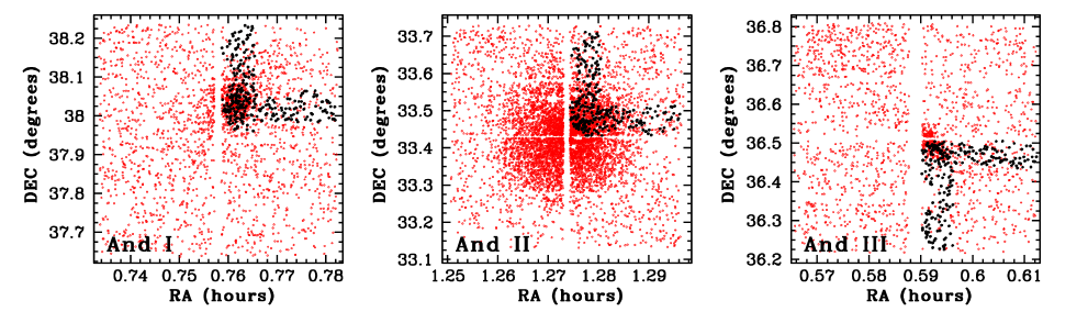
Figure 1.— The distribution of stars from the KPNO wide-field Mosaic observations of each dSph are shown as small points. The selection function used to isolate these stars involved a simple cut on the color-magnitude diagram (CMD) to enhance the dSph RGB with respect to the field population, which is still abundantly present in the maps. Superimposed on the photometric data are the objects targeted with Keck/DEIMOS spectroscopy (darker points).

2. The Data Set

The imaging and spectroscopic observations for three of the six dSphs in this study are being presented for the first time (And I, II, and III), whereas the data sets for And VII, X, and XIV have been (at least partially) presented in previous studies. For these three galaxies, however, we present a new analysis of the spectra in the present paper. We begin by first introducing the new data for And I, II, and III, followed by a short summary of the previously presented data for And VII, X, and XIV, including any relevant new analysis.

2.1. Photometric and Spectroscopic Observations – And I, II, and III

We imaged each of And I, II, and III with the wide-field Mosaic camera on the Kitt Peak National Observatory (KPNO) 4-m telescope from 1998 to 2002 (Ostheimer 2003). This camera subtends an angular size of 36${}^{\prime}\times$ 36^′, much larger than the King limiting diameter of And I ($r_{l}$ = 10.4^′) and And III ($r_{l}$ = 7.2^′), and slightly smaller than that of And II ($r_{l}$ = 22.0^′). The observations were obtained in the Washington System ($M$, $T_{2}$) bands and converted to Johnson-Cousins ($V$, $I$) using the relations given in Majewski et al. (2000). The exposure times were set at 900 seconds in the $M$ filter and 3,600 seconds in the $T$ filter, reaching a photometric depth of $I\sim$ 24. The most luminous (metal-poor) RGB stars have intrinsic magnitudes of $M_{I}$ $\sim$ $-$4, and therefore at the distance of M31 (780 kpc, ($m-M$)₀ = 24.5), these stars will have $I_{\rm 0}$ = 20.5. Our imaging observations are therefore well suited to probe several magnitudes of the RGB in each of the dSphs.

We also obtained imaging observations of the same fields using the intermediate-width $DDO51$ filter (Majewski et al., 2000). This filter is centered on the surface-gravity sensitive Mgb and MgH stellar absorption features, and therefore provides an efficient means to discriminate foreground Milky Way contaminants from M31 dSph RGB stars (Ostheimer, 2003; Gilbert et al., 2006; Guhathakurta et al., 2006). The filter is especially efficient at boosting our odds of targeting true dSph stars that are located far from the core of each galaxy, where the surface brightness of members if low relative to the foreground veil of Milky Way dwarf stars. These stars, in the outskirts of the dSphs, represent key data points when studying radial trends. The combination of the wide-field broadband imaging observations with co-spatial $DDO51$ filter exposures provides the necessary framework to conduct the first largely uncontaminated study of the properties of M31 dSphs.

With this unique photometric data set in hand, we spectroscopically targeted the brightest RGB candidates in each of And I, II, and III with the DEIMOS multiobject spectrograph (Faber et al., 2003) on the Keck II 10-meter telescope. To do this, we first measured the positions of all stars in the KPNO Mosaic images and transformed the positions into equatorial coordinates using the USNO-B Guide Star Catalogue as a reference (Monet et al., 2003). These positions were then mapped onto the DEIMOS mask. The spectroscopic data were collected in late 2005, as summarized in Table 1. The observations were obtained using the standard setup described in detail in several previous papers (e.g., Gilbert et al. 2006, Guhathakurta et al. 2006 and Kalirai et al. 2006b). To summarize a few key details, the spectroscopic observations were obtained using the 1200 lines mm^-1 grating at a central wavelength of 7800 ${\rm\AA}$. The resolution of the spectra for a typical seeing of 0$\farcs$8 FWHM is 1.3 ${\rm\AA}$ and the spectral range is $\approx$6400 – 9100 ${\rm\AA}$, depending exactly on the position of each object relative to the mask center.

In total, we measured a spectrum for 835 objects in six masks (two per galaxy), where each mask subtends roughly 16${}^{\prime}\times$ 4^′. Of these, 42 objects were measured on multiple masks to assess our radial velocity accuracy (see § 2.3). The targets were chosen over a magnitude range extending from just above the tip of the RGB down to $\sim$2 magnitudes below the tip in each satellite. The mean spectral $S/N$ in the entire sample of observations is $\sim$5 per pixel. The $DDO51$ filter observations were used to screen objects in the selection process to ensure that high probability RGB stars were targeted before lower probability objects (which turn out to be mostly foreground Milky Way dwarfs).

The positions and orientations of the Keck/DEIMOS spectroscopic fields relative to And I, II, and III were carefully placed to allow both a study of stars near the center of each dSph and also to probe radially outward from the core. To illustrate these pointings, we present starcount maps of each galaxy taken from our wide-field KPNO Mosaic imaging data in Figure 1. For each galaxy, we make a very rough cut on the photometric data to isolate stars located along the RGB in the color-magnitude diagrams (CMDs), which are presented later in § 3. The spectroscopic targets are shown as darker points.

2.1.1 Existing Observations of And VII, X, and XIV

The data sets for And VII, X, and XIV differ from the three dSphs discussed above in several ways, and so we briefly summarize this sample here. First, for And VII, the photometry was obtained by Grebel & Guhathakurta (1999) using Keck/LRIS. The galaxy is one of the most luminous M31 satellites known, with an integrated brightness of $M_{\rm V}$ = $-$13.3 $\pm$ 0.3, and so several of the brightest red giants in the photometric sample were targeted with Keck/HIRES for spectroscopy. These observations utilized special purpose multislit masks with a half dozen slitlets each, with each slitlet having a length of 1 – 2$\farcs$5. The technique employed is described in detail in Sneden et al. (2004), in the context of similar observations of the globular cluster M3. Note, Grebel & Guhathakurta (1999) refer to this galaxy as the Cassiopeia dSph in their paper.

The second galaxy in this existing sample is And X, a newly discovered low-luminosity M31 dSph from the Sloan Digital Sky Survey (Zucker et al., 2007). We used the imaging data set described by Zucker et al. (2007) to target two Keck/DEIMOS spectroscopic masks in this galaxy, using the same setup as discussed above (and below) for And I, II, III. The details of the observations, data reduction, and results are presented in Kalirai et al. (2009).

The final galaxy in the sample is And XIV, a system that we discovered with KPNO/Mosaic three years ago. This galaxy is one of the most remote systems known in M31, located at a projected distance of 162 kpc and a line of sight distance that places it behind M31 by $\sim$80 kpc. We targeted And XIV with two Keck/DEIMOS spectroscopic masks, again, using an identical setup as discussed above (and below) for And I, II, and III. The details of the observations, data reduction, and results for this dSph are presented in (Majewski et al., 2007).

2.2. Data Reduction

Data reduction of the six DEIMOS multi-slit masks being presented for the first time in the present study (And I, II, and III) are based on the spec2d software pipeline (version 1.1.4) developed by the DEEP2 Galaxy Redshift Survey team at the University of California-Berkeley for that project (see Faber et al. 2007 for more information). Briefly, internal quartz flat-field exposures are obtained and used to rectify the curved raw spectra into rectangular arrays by applying small shifts and interpolating in the spatial direction. A one-dimensional slit function correction and two-dimensional flat-field and fringing correction are applied to each slitlet. Using the DEIMOS optical model as a starting point, a two-dimensional wavelength solution is determined from multiple Kr-Ar-Ne-Xe arc lamp exposures with residuals of order 0.01 ${\rm\AA}$. Each slitlet is then sky-subtracted exposure by exposure using a B-spline model for the sky. The individual exposures of the slitlet are averaged with cosmic-ray rejection and inverse-variance weighting. Finally one dimensional spectra are extracted for all science targets using the optimal scheme of Horne (1986) and are rebinned into logarithmic wavelength bins with 15 km s^-1 per pixel. We note that the modifications to this pipeline discussed by Simon & Geha (2007) and Gilbert et al. (2009) were used in the present reductions. Specifically, the cosmic ray rejection algorithm was altered to allow alignment of individual two dimensional exposures in the spatial direction before co-addition.

In Figure 2, we present several of our final 1-dimensional spectra for stars in each of the three M31 dSphs. Only a 500 ${\rm\AA}$ section of the spectrum centered near the Ca ii triplet is shown in each case for the sake of clarity. These absorption lines, as well as other spectral features, are clearly visible in the data for bright and faint objects in each galaxy.

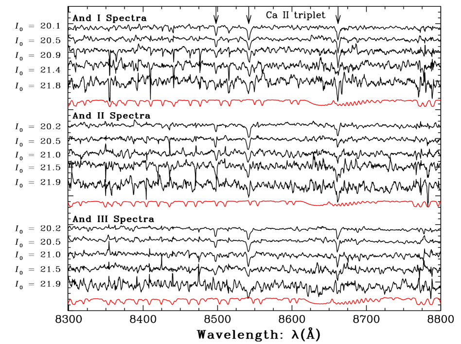
Figure 2.— Five sample spectra of RGB stars in And I, II, and III corrected to zero velocity. To illustrate the quality of the full data set, these spectra have been chosen over a magnitude range extending from the brightest to the faintest stars in our spectroscopic sample. The wavelength window of 500 ${\rm\AA}$ has been centered near the Ca ii triplet absorption lines (8498, 8542, and 8662 ${\rm\AA}$) which are clearly detected in all objects. The red curve curve shows a sample inverse variance spectrum for each dSph, calculated under the assumption that the errors are dominated by Poisson statistics in the sky+object counts, and intended to help distinguish between real features (e.g., Ca ii triplet absorption lines) and noise artifacts for the faintest stars plotted. The full spectral coverage of these data is $\sim$2,700 ${\rm\AA}$, which allows multiple features to be used in the cross-correlation to yield accurate radial velocities. The spectra have been smoothed using a 7 pixel boxcar function for illustration purposes only.

2.3. Radial Velocity Measurements

Radial velocities are measured for all extracted one-dimensional spectra by cross-correlating the observations with a series of high signal-to-noise stellar templates. The stellar templates were observed using the same DEIMOS setup described above, and range in spectral type from F8 III to M8 III, and also include subgiants and dwarfs. For the faintest objects with lower signal-to-noise, this cross-correlation does not yield meaningful results and therefore we manually check all of the template fits and only include those spectra in which the template matched at least two different spectral features (see Guhathakurta et al. 2006 for more details). Of the initial sample of 835 spectra, this left 426 spectra after eliminating galaxies, 148 in And I, 136 in And II, and 142 in And III. These numbers include 1 duplicate in the And I observations, 1 in And II, and 8 in And III. The duplicates represent observations of the same star on both masks, where both spectra yielded a reliable velocity measurement from the cross correlation.

Below the set of sample spectra for each dSph in Figure 2 is shown the inverse of the variance spectrum (red), computed under the idealized assumption that it is dominated by Poisson statistics in the sky+object counts. The spectral measurements presented in this paper—the cross-correlation analysis used to measure radial velocities and the measurement of absorption line strengths (see § 5.2)—properly take into account this dependence of the uncertainty in the spectral flux on wavelength. The dips in the inverse variance spectrum correspond to bright night sky emission lines, shifted in wavelength to account for the shift in the science spectra from the observer frame to the rest frame. Occasionally, systematic errors in sky subtraction can cause the actual uncertainty to be greater than the Poisson errors shown here. The inverse variance spectra are plotted to help the reader distinguish between real features (e.g., the Ca ii triplet absorption lines) and noise artifacts for the fainter stars in our sample.

The uncertainties in our velocity measurements are empirically estimated to be $\sim$10 km s^-1, based on the comparison of independent observations from these duplicates. While this uncertainty is many times less than the velocity dispersion in bulge and halo-like populations, it is comparable to, if not larger than, the expected velocity dispersion in small dSphs. A significant fraction of the radial velocity uncertainty budget derives from random and systematic astrometric errors. As discussed earlier, in designing our spectroscopic masks we used the USNO-B Guide Star Catalogue to calculate absolute positions of all stars. The internal accuracy of this catalogue is known to be $\sim$0$\farcs$2 (Monet et al., 2003). At the DEIMOS pixel scale (0$\farcs$1185 per pixel), this uncertainty alone translates to 1.7 pixels. Given that the dispersion of the 1200 lines mm^-1 grating is 0.33 ${\rm\AA}$ pixel^-1 and the anamorphic factor is 0.6 at 8000 ${\rm\AA}$, a 1.7 pixel uncertainty results in a 0.3 ${\rm\AA}$ wavelength uncertainty. Therefore, a random misalignment of the centroid of a star by 0$\farcs$2 in the slit can lead to a velocity error of 12 km s^-1. The positional accuracy of a given target will also depend on the overall solution of the astrometric transformation and therefore depends on the density of astrometric reference stars available at a particular location in the imaging frame. Finally, we note that a number of other effects can also lead to uncertainties in the astrometry. These can include positional uncertainties in the images (e.g., if one or more reference stars have an appreciable proper motion), slight imperfections in the mechanical cutting process that produces the slits, and even small misalignments (i.e., rotations or shifts) of the entire mask during the observations.

Fortunately, these astrometric uncertainties leave a signature that can be used to calculate the amount that the radial velocity measurement is offset from the true value. This method, as discussed by Sohn et al. (2007) and Simon & Geha (2007), utilizes atmospheric absorption features that are superimposed on the stellar spectra. The strongest of these telluric lines are in the A-band (7600 – 7630 ${\rm\AA}$). To correct for the mis-centering, we observed several bright, rapidly rotating, hot standard stars with few emission or absorption lines (e.g., the Wolf Rayet star Wolf1346). The near featureless spectra of these stars displays a very clean detection of the A-band absorption. The telluric templates were created by allowing these stars to drift perpendicularly across the slit during each short exposure, ensuring that the starlight evenly fills the slit. Next, we averaged the spectra for all such standards and cross-correlated a windowed region of the coadded spectra at the wavelength of the A-band absorption to the observed stellar spectra. For a star that is perfectly centered in the slit, this cross-correlation produces a near perfect match indicating that no offset is required. However, for a star that is mis-centered in the slit, the observed wavelength of the A-band is offset relative to the standard star template. We use this offset to calculate a velocity shift and apply this correction to each of our 426 radial velocities. The mean offset for each mask ranged from 0.7 – 10.2 km s^-1, with a standard deviation of 5 – 13 km s^-1. The final addition to each of our velocity measurements includes a heliocentric correction to convert our geocentric velocities into a heliocentric frame of reference.

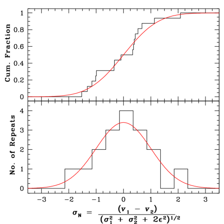
Figure 3.— Repeat measurements of the same stars in our And I, II, III, and X data sets are used to define a normalized error, $\sigma_{N}$ equal to the ratio of the difference in velocity of the duplicates and the quadrature sum of all error terms. In addition to the Monte Carlo error estimates, we find that an additional error ($\epsilon$) is needed to reproduce a unit Gaussian in the resulting distribution of $\sigma_{N}$ (solid histogram). As discussed in § 2.4, we formally add $\epsilon$ = 2.2 km s^-1 in quadrature to each of our radial velocity errors to match the results from Simon & Geha (2007), which are based on a much larger sample of repeat measurements taken with a similar setup to this work.

2.4. Radial Velocity Uncertainties

The observed velocity dispersions of the M31 satellites in this study reflect a combination of the actual intrinsic dispersions, plus the velocity errors. The known intrinsic dispersion of other Local Group satellites are often 5 – 10 km s^-1, which is comparable to the expected errors in our velocity measurements. It is therefore very important to have a good understanding of the true uncertainties in our measurements. We measure these uncertainties using a Monte Carlo method, where we first take each stellar spectrum and add noise to each pixel scaled by the estimated variance in that pixel (also see discussion in Simon & Geha 2007). This procedure is repeated 1000 times assuming the variance in each pixel is distributed according to Poisson statistics, and the velocity and telluric correction is re-calculated after each run of the simulation. The error in the velocity ($\sigma$) is defined as the square root of the variance in the recovered mean velocity.

We next compare this error measurement to the known uncertainty, measured as the difference in velocity between independent measurements of the same star (e.g., $v_{1}$ and $v_{2}$). For this, we use the 10 duplicates with reliable velocity measurements in this data set, as well as the 7 duplicates in our And X data set (Kalirai et al., 2009). For these stars, we define a normalized error, $\sigma_{N}$, as the ratio of the velocity difference between duplicate measurements and the quadrature sum of all error contributions ($\sigma_{1}$, $\sigma_{2}$, and $\sqrt{2}$$\epsilon$). The latter includes the Monte Carlo errors in each of the two velocity measurements, as well as an additional term representing any other error that we have not accounted for. The distribution of $\sigma_{N}$ for all duplicates is shown in Figure 3, and in order to reproduce a unit Gaussian, we measure $\epsilon$ to be $\lesssim$3 km s^-1. For our final velocity errors, we choose to formally add an $\epsilon$ of 2.2 km s^-1 in quadrature with the Monte Carlo errors. Although our measured value is slightly larger than this, 2.2 km s^-1 reflects the $\epsilon$ measured by Simon & Geha (2007) from a similar Keck/DEIMOS study, but with a factor of three larger data set of duplicate measurements. With only 17 data points, our measured $\sigma_{N}$ is much more susceptible to a few outliers than their sample. We note that the resulting velocity errors from this analysis, and with this value of $\epsilon$, have been directly tested by Simon & Geha (2007) by comparing to high dispersion observations of a Milky Way globular cluster and dSph galaxy, each with velocity uncertainties of $<$1 km s^-1. The results from the Keck/DEIMOS analysis are in excellent agreement ($<$1$\sigma$) with the high resolution studies.

Figure 4.— The total uncertainty in our velocity measurements for all stars along the sightline to And I, II, and III is shown as a function of the mean spectral $S/N$ per pixel. The uncertainties reflect both random and systematic velocity error contributions, the two being added in quadrature as discussed in § 2.4. Even for spectra with $S/N$ = 5, we are able to measure velocities accurately to $\sigma_{v}$ = 4 km s^-1.

In Figure 4 we present the final error distribution of all velocity measurements in our data set, as a function of the spectral $S/N$ (per pixel). As expected, the highest $S/N$ stars have a velocity error equal to the “floor” established above (2.2 km s^-1) whereas the error increases to $\sim$4 km s^-1 for stars with $S/N$ = 5, and quickly increases for lower $S/N$ spectra. The median uncertainty across the full sample is 4.4 km s^-1.

Figure 5.— The velocity histograms of And VII (left – Guhathakurta, Reitzel, & Grebel 2000), And X (middle – Kalirai et al. 2009), and And XIV (right – Majewski et al. 2007). The properties of each of these satellites, as measured from these kinematical data, are discussed in the text.

We stress that the analysis presented above in carefully understanding the velocity errors in these data is essential to accurately probe the internal kinematics of dwarf galaxies. The uncertainty introduced by even very small astrometric errors (e.g., at the 0$\farcs$05 – 0$\farcs$1 level) in the centroids of targets leads to radial velocity uncertainties that are larger than the dispersions of some satellites. Furthermore, these uncertainties, for a given spectrum, systematically offset the wavelengths of all spectral features by the same amount. The rms scatter between velocity measurements, as measured from different absorption lines, can therefore not provide an accurate assessment of the overall uncertainty in radial velocity.

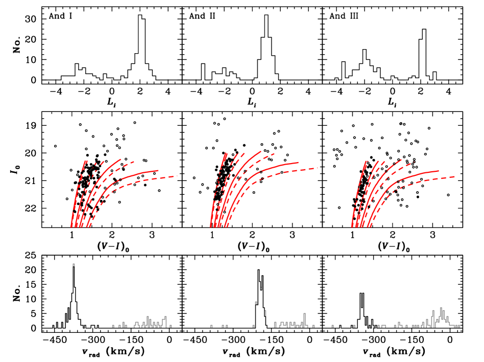
Figure 6.— Top – The distribution of likelihoods of individual stars being giants at the distance of M31 ($L_{i}>$ 0) or foreground Milky Way dwarfs ($L_{i}<$ 0) for each of our And I, II, and III sightlines. The likelihoods are constructed using five different photometric and spectroscopic diagnostics as discussed in § 3 and Gilbert et al. (2006). We consider the giants to be those stars that are three times more likely to be M31 giants as compared to Milky Way dwarfs ($L_{i}$ $\geq$ 0.5). Middle – CMDs for And I, II, and III illustrating our giant (filled points) and dwarf (open points) stars. The giants clearly form a tight RGB that follows the most metal-poor isochrones shown (see text). The filled points with redder colors that do not follow the locus of most giants are field M31 halo stars, as discussed in § 3. Bottom – Radial velocity histograms for each of our And I, II, and III sightlines show a dominant cold population at large negative velocities (the dSphs) as well as a smaller underlying broad distribution (M31 field halo RGB stars). Foreground Milky Way dwarfs are also seen at small velocities and are well separated from the dSph stars. The grey histogram shows all stars for which we measured a velocity whereas the black histogram illustrates our giant sample (dSph members and M31 field halo stars). As discussed in § 3, the And I sightline is contaminated by M31 field substructure with a similar velocity to the dSph. This substructure is present in this Figure, and is removed to create our final member dSph RGB sample as illustrated in Figure 7.

2.5. Radial Velocity Measurements for
And VII, X, and XIV

The method used to reduce the And X and XIV Keck/DEIMOS spectroscopic data, including the measurement of radial velocity and uncertainty, is very similar to the description above and has been presented in Kalirai et al. 2009 and Majewski et al. 2007). For And VII, the Keck/HIRES data were analyzed slightly differently. The sky subtraction was performed by combining the few pixels of sky in all of the slits into a master sky spectrum. The velocities were extracted by cross correlating the And VII target spectra with radial velocity standard stars. The latter were observed through the same slitlets on the same HIRES masks as the science observations. Although the $S/N$ of the spectra are quite low, the wide baseline in wavelength allowed reliable velocities to be measured for 18 of the 21 And VII RGB candidates. The uncertainties in the individual velocity measurements are $\lesssim$1.5 km s^-1.

3. Establishing Member Stars in Each dSph

Membership of stars in the three previously observed dSphs, And VII, X, and XIV, have been discussed in Guhathakurta, Reitzel, & Grebel (2000), Kalirai et al. (2009), and Majewski et al. (2000), and so we refer to those papers for the details (the analysis of And X and XIV is identical to the discussion below). Summarizing, accurate radial velocities and uncertainties were established for 18 member stars in And VII, 22 member stars in And X, and 38 member stars in And XIV. These papers, as well as Grebel & Guhathakurta (1999), present the CMDs for each of these satellites. We summarize the three radial velocity histograms for these galaxies in Figure 5, and now focus on the new observations of And I, II, and III.

In section 1 we noted that only one previous spectroscopic study of stars in And I and And III exists (Guhathakurta, Reitzel, & Grebel, 2000), and two such studies of And II exist, both being based on the same data set (Cote, Oke, & Cohen, 1999; Cote et al., 1999). For And I and III, Guhathakurta, Reitzel, & Grebel (2000) were able to measure velocities for 29 and 7 dSph member stars, respectively, but with large velocity errors. Cote, Oke, & Cohen (1999) established accurate radial velocities for seven member stars in And II and confirmed 35 other members with very poor radial velocity accuracy, $\sigma_{v}>$ 40 km s^-1 (Cote et al. 1999b; P. Cote 2006, private communication). The first aim of our survey is to significantly increase the numbers of stars with accurate radial velocities ($\sigma_{v}\lesssim$ 10 km s^-1) in these galaxies. In Figure 6 (bottom), we present radial velocity histograms for all objects for which we could measure a velocity as discussed earlier (grey histogram). For each of our And I, II, and III fields, there is a very clean detection of a kinematically cold spike representing stars that belong to the dSph. We also see a small population of field M31 stars with a broad range of velocities. Considering that each of And I, II, and III are located well beyond the radius at which M31’s halo dominates its inner spheroid (25 – 30 kpc, Guhathakurta et al. 2005; Kalirai et al. 2006a), these field stars likely represent M31 halo members. Finally, there is a population of foreground Milky Way dwarf stars at small negative velocities.

We establish membership of stars belonging to And I, II, and III using a three step process. This involves first isolating the sample of stars that have characteristics of giants at the distance of M31, second, eliminating any M31 substructure, and, third, cleaning the dSph populations of any M31 field stars in the halo. For the first cut, we can use photometric and spectroscopic diagnostics to remove any Milky Way dwarf stars along the line of sight. The diagnostics used for this separation include radial velocity measurements, $DDO51$ photometry, strength of the Na i doublet, position of the star in the CMD, and a comparison of the photometric and spectroscopic metallicities of each star. Details on the resolving power of each of these diagnostics to weed out Milky Way dwarf star contamination, as well as a careful step-by-step cookbook on how they are applied to the data set, are presented in Gilbert et al. (2006). As those methods were developed to separate out stars in M31’s (kinematically hot) field halo from Milky Way contaminants, we note that we made two small changes in this application. First, the velocity and dispersion of the expected dSph stars were set to the rough values of the peaks in Figure 6, and second the distance of each satellite (e.g., in calculating a photometric metallicity) was set to the known distances of And I (745 $\pm$ 24 kpc), And II (652 $\pm$ 18 kpc), and And III (749 $\pm$ 24 kpc) as reported in McConnachie et al. (2005). The uncertainty in the adopted distance of each satellite produces a very small effect on the overall classifications, given both the nature of the measurement and the relative insensitivity of the two affected diagnostics (i.e., metallicity comparison and position in the CMD) compared to others (e.g., radial velocity and $DDO51$ photometry). The final likelihoods of a star being a giant or dwarf are illustrated in the top panel of Figure 6; values of $L_{i}$ that are positive are more likely to be giants and values with $L_{i}$ $<$ 0 are likely Milky Way dwarfs. Our final selection of giants are those stars that are three times more likely to be giants than Milky Way dwarfs (corresponding to $L_{i}$ $\geq$ 0.5), as discussed in Gilbert et al. (2006) and Kalirai et al. (2006a).

The distribution in radial velocity of giant stars in fields And I, II, and III are shown as the solid histogram in Figure 6 (bottom). Clearly, this separation has removed the obvious Milky Way dwarf stars at small negative velocities, however, we note that a few dwarf outliers are also removed at (or close to) the velocity of the dSph satellites. The distribution of the M31 giants (filled points) and Milky Way dwarfs (open points) are also shown on the CMD in Figure 6 (middle panels). The giants form a tight sequence in the CMD, stretching from the tip of the RGB to our photometric limit at $I_{\rm 0}\sim$ 22, whereas the dwarf stars occupy a broad range in color and luminosity depending on their spectral type and distance. The three solid red curves on these diagrams are theoretical isochrones for an age of 12 Gyr and [$\alpha$/Fe] = 0.0, with a metallicity of [Fe/H] = $-$2.31 (left), $-$1.31, and $-$0.83, and $-$0.40 (right) from the Vandenberg, Bergbusch, & Dowler (2006) models. The dashed curves are the same isochrones assuming [$\alpha$/Fe] = +0.3. As we will quantify in § 5.3, each of these dSphs appear to contain a metal-poor population of stars with a modest dispersion.

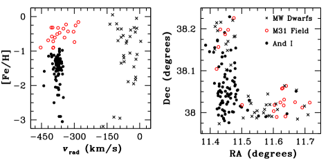
Figure 7.— The And I dSph is spatially located within identified halo substructure from the Giant Southern Stream (Ibata et al., 2007; Gilbert et al., 2009). Left – The substructure is isolated from the dSph stars with a metallicity cut, where the more metal-rich material is associated with the stream debris. Right – As expected, these stars, shown as red open circles, are also located in the outskirts of our spectroscopic masks which intersect at the center of And I.

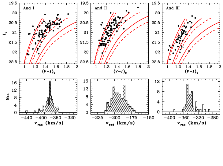
Figure 8.— A closer view of the CMD (top) and radial velocity histograms (bottom) for our final And I (80 stars), And II (95 stars), and And III (43 stars) samples of RGB members (filled points and histograms). Open points and histograms show the M31 field halo giant stars that are eliminated from the final sample as discussed in § 3. The three sets of isochrones shown in each panel of the CMDs are taken from Vandenberg, Bergbusch, & Dowler (2006), for an age of 12 Gyr and metallicities of [Fe/H] = $-$2.31 (left), $-$1.31 (middle), and $-$0.83 (right), and have been shifted to each satellites’ distance modulus. The models for [$\alpha$/Fe] = 0.0 are shown as solid curves and those for [$\alpha$/Fe] = +0.3 are shown as dashed curves. Clearly, all three of these satellites are metal-poor systems.

The second cut in our membership criteria only applies to And I, which is situated at a spatial location in M31 that appears to contain substructure related to the Giant Southern Stream (Ibata et al., 2007). As Gilbert et al. (2009) show, the substructure in this field is located at roughly the same velocity as And I, but is much more metal-rich than the dSph stars. We can see the substructure in the CMD of this dSph as an extention of metal-rich stars. This is illustrated more clearly in Figure 7, where we show the M31 giants (circles) and Milky Way dwarfs (crosses) in the And I field on an [Fe/H] vs $v_{\rm rad}$ plane (left panel – see § 5.3 for the details on how [Fe/H] is calculated). The reported photometric metallicity of the Milky Way dwarfs is meaningless since their distance is unknown. However, the metallicity of And I and the stream contamination is correct since these populations are both located at M31’s distance. The diagram shows a bi-modality with a split at [Fe/H] $\sim$ $-$0.9, where the bulk of the And I stars (filled points – see below) comprise the more metal-poor, tight grouping of stars. To further illustrate that the metal-rich stars in this diagram are likely not members of And I, we look at their positions relative to our two spectroscopic masks in the right panel. As expected, the stars associated with the stream contamination are found in the outskirts of the masks, far from And I, where the densities of the dSph and the field become more equal. We note that the King limiting radius of the dSph is 10^′, and most of these stars are located beyond this radius. Formally, we have selected the exact cut that separates the filled circles from the open circles arbitrarily at the apparent break point in Figure 7 (left). For our sample, this translates to a hard cut of [Fe/H] $<$ $-$0.92 for the And I members, although we recognize that the exact separation may be slightly shifted from this value and depends on the relative age and distance difference between the two populations. The hard cut may also lead to the truncation of any metal-rich tail in the dSphs metallicity distribution function.

The final cut in our membership criteria eliminates any likely M31 field halo giants not associated with each dSph. The limiting radii of And I is 10.4^′, of And II is 22.0^′, and of And III is 7.2^′ (McConnachie & Irwin, 2006), and so we eliminate three stars in And I and eight stars in And III that are located beyond these limits. These eliminations work to actually remove stars that can be easily identified as outliers on the velocity histograms. For example, in And I one of the stars eliminated has a radial velocity of $-$440.0 km s^-1, and in And III one of the stars is moving at $v_{\rm rad}$ = $-$431.6 km s^-1. Both of these stars have velocities that are 5 – 10$\sigma$ deviant from the final observed dispersion. Additionally, the cut at the limiting radius in And III eliminates the two giants with $V{\rm-}I$ $>$ 2 in the CMD in Figure 6. The photometric metallicity of these two stars is calculated to be [Fe/H] $>$ $-$0.25, well over 10 times more metal-rich than the remaining dSph stars (see § 5.1). The resulting velocity distribution still includes M31 field halo giants that are spatially superimposed on the dSph population. To eliminate these last few stars, we measure the mean and sigma of the resulting velocity distribution and iteratively eliminate stars that are more than 3-$\sigma$ from the mean. This iteration removes just two stars from And I, zero stars from And II, and three stars from And III’s sightline. The eliminated stars were again not centrally located in the dSph suggesting they are likely field halo giants. The final selected members of these three dSphs include 80 stars in And I, 95 stars in And II, and 43 stars in And III.

We stress that our primary goal from the selection process described above is to construct as secure a sample as possible of confirmed RGB members of these three satellites. Given the cuts used, it is possible (although unlikely) that we have in fact thrown a member or two out of the sample, however our sample sizes are large enough that the exclusion of a few stars will not impact the analysis that follows. The filled histograms in Figure 8 (bottom) illustrate the velocities for the stars in the final sample, and the filled points in the top panel of this Figure show their distribution in the CMD. The open histograms (bottom) and open points (top) in Figure 8 represent the eliminated giants from the limiting radius and $\sigma$-clipping cuts discussed above.

4. Mean Velocities, Intrinsic Velocity Dispersions, and $M/L$ Ratios

We calculate the mean radial velocity and intrinsic dispersion for each of the six dSphs using the maximum-likelihood method described by Walker et al. (2006). This method assumes that the observed dispersion is the sum of the true intrinsic dispersion and the velocity errors discussed at length in § 2.4. For And I, we find $v_{\rm rad}$ = $-$375.8 $\pm$ 1.4 km s^-1 and $\sigma_{v}$ = 10.6 $\pm$ 1.1 km s^-1, for And II we find $v_{\rm rad}$ = $-$193.6 $\pm$ 1.0 km s^-1 and $\sigma_{v}$ = 7.3 $\pm$ 0.8 km s^-1, for And III we find $v_{\rm rad}$ = $-$345.6 $\pm$ 1.8 km s^-1 and $\sigma_{v}$ = 4.7 $\pm$ 1.8 km s^-1, for And VII we find $v_{\rm rad}$ = $-$309.4 $\pm$ 2.3 km s^-1 and $\sigma_{v}$ = 9.7 $\pm$ 1.6 km s^-1, for And X we find $v_{\rm rad}$ = $-$168.3 $\pm$ 1.2 km s^-1 and $\sigma_{v}$ = 3.9 $\pm$ 1.2 km s^-1, and for And XIV we find $v_{\rm rad}$ = $-$481.0 $\pm$ 1.2 km s^-1 and $\sigma_{v}$ = 5.4 $\pm$ 1.3 km s^-1. The mean radial velocities of these six galaxies are consistent with M31 membership, since M31 has a systemic velocity of $-$300 km s^-1. The one exception to this may be And XIV, which has both a large negative radial velocity and a large distance from M31 (both projected and along the line of sight). As discussed in Majewski et al. (2007), the galaxy may therefore be falling into the Local Group for the first time. The velocities for And I and II are inconsistent with the measurements by previous studies within the mutual 1-$\sigma$ errorbars established by this and the previous studies (Guhathakurta, Reitzel, & Grebel, 2000; Cote et al., 1999). As we noted earlier, these previous results are only based on a handful of stars and therefore our values are much more secure. For And III, Guhathakurta, Reitzel, & Grebel (2000) found $v_{\rm rad}$ = $-$352.3 $\pm$ 13.6 km s^-1 based on 9 RGB members, which is consistent with our much more precise result.

The central velocity dispersion of the six galaxies in this study varies by more than a factor of 2.5. The only previous measurement to compare our results with is the high resolution study of Cote et al. (1999), which established $\sigma_{v}$ = 9.3 $\pm$ 2.7 km s^-1 for And II based on seven RGB stars. Our result is consistent within the larger error bar determined by Cote et al. (1999) for their measurement, however we find that the velocity dispersion is lower. We can use our new velocity dispersions to put first order constraints on the total mass (stellar and dark matter) of each satellite using the method described by Illingworth (1976), $M$ = 167*$\beta$$r_{c}$$\sigma_{v}^{2}$ where $\beta$ = 8 for dSphs (Mateo, 1998). This formalism was initially constructed for the analysis of line of sight velocities in globular clusters and therefore has several assumptions built into it, all of which may not be true. For example, we are assuming the galaxies are spherical, are in dynamical equilibrium, and have an isotropic velocity dispersion. We are also assuming that the stellar distribution follows a King profile (which is observed) and traces the dark matter. We return to a discussion on how more accurate dynamical mass measurements can be established for M31 dSphs below.

The core radius of four of the six dSphs is known from the structural study of McConnachie & Irwin (2006), who find $r_{c}$ = 580 $\pm$ 60 pc for And I, $r_{c}$ = 990 $\pm$ 40 pc for And II, $r_{c}$ = 290 $\pm$ 40 pc for And III, and $r_{c}$ = 450 $\pm$ 20 pc for And VII (geometric means). The measured core radius, and an assumed 10% uncertainty, of And X is $r_{c}$ = 270 $\pm$ 30 pc (Zucker et al. 2007) and that of And XIV is much larger at $r_{c}$ = 730 $\pm$ 70 pc (Majewski et al. 2007). The total masses of these satellites are therefore $M$ = (8.7 $\pm$ 1.6) $\times$ 10⁷ $M_{\odot}$ for And I, $M$ = (7.0 $\pm$ 1.1) $\times$ 10⁷ $M_{\odot}$ for And II, $M$ = (8.6 $\pm$ 4.8) $\times$ 10⁶ $M_{\odot}$ for And III, $M$ = (5.7 $\pm$ 1.3) $\times$ 10⁷ $M_{\odot}$ for And VII, $M$ = (5.5 $\pm$ 2.5) $\times$ 10⁶ $M_{\odot}$ for And X, and $M$ = (2.9 $\pm$ 1.0) $\times$ 10⁷ $M_{\odot}$ for And XIV. At the luminous end, for $M_{\rm V}$ = $-$11 to $-$13, the masses of And I, II, and VII are similar to Milky Way dSphs (e.g., Fornax and Leo I), calculated in the same way. At lower luminosities, the masses of And III and X appear to be lower than systems in the Milky Way with similar brightness, such as Carina, Draco, and Sextans.

We can calculate the mass-to-light ratios in Solar units of And I, II, III, VII, X, and XIV by combining the masses determined above with the measured luminosities of each satellite (see McConnachie & Irwin 2006; Zucker et al. 2007; Majewski et al. 2007). This gives $M/L_{\rm V}$ = 19 $\pm$ 4 for And I, $M/L_{\rm V}$ = 7.5 $\pm$ 1.8 for And II, $M/L_{\rm V}$ = 8.3 $\pm$ 5.2 for And III, $M/L_{\rm V}$ = 3.2 $\pm$ 1.2 And VII, $M/L_{\rm V}$ = 37 $\pm$ 24 for And X, and $M/L_{\rm V}$ = 160 $\pm$ 95 for And XIV. The mass-to-light ratios indicate that these satellites are dark matter dominated, as expected, however both And II and III are at the low end of the range of $M/L$ ratios for dSphs. A more in depth comparison of the results in this section, as well as their implications, will be presented in § 6.4.

In Table 2 we summarize several of the fundamental properties of each of the six satellites discussed above. This includes their luminosities, projected distance from M31, mean radial velocities, intrinsic velocity dispersions, metallicities, and metallicity dispersions (see § 5 for half-light radii, total masses, and $M$/$L$ ratios). Further details on the individual galaxies are also available in the Guhathakurta, Reitzel, & Grebel (2000), Kalirai et al. (2009), and Majewski et al. (2007) studies.

Table 2

Property	And I	And II	And III	And VII	And X	And XIV
$M_{\rm V}$	$-$11.8 $\pm$ 0.1	$-$12.6 $\pm$ 0.2	$-$10.2 $\pm$ 0.3	$-$13.3 $\pm$ 0.3	$-$8.1 $\pm$ 0.5	$-$8.3 $\pm$ 0.5
$R_{\rm proj}$ (kpc)	44.9	145.6	68.2	214.5	75.5	162.5
$v_{\rm rad}$ (km s-1)	$-$375.8 $\pm$ 1.4	$-$193.6 $\pm$ 1.0	$-$345.6 $\pm$ 1.8	$-$309.4 $\pm$ 2.3	$-$163.8 $\pm$ 1.2	$-$481.0 $\pm$ 2.0
$\sigma_{v}$ (km s-1)	10.6 $\pm$ 1.1	7.3 $\pm$ 0.8	4.7 $\pm$ 1.8	9.7 $\pm$ 1.6	3.9 $\pm$ 1.2	5.4 $\pm$ 1.3
[Fe/H]	$-$1.45 $\pm$ 0.04	$-$1.64 $\pm$ 0.04	$-$1.78 $\pm$ 0.04	$-$1.40 $\pm$ 0.30	$-$1.93 $\pm$ 0.11	$-$2.26 $\pm$ 0.05
$\sigma_{[Fe/H]}$	0.37	0.34	0.27	$\cdots$	0.48	$\cdots$
$r_{c}$	580 $\pm$ 60	990 $\pm$ 40	290 $\pm$ 40	450 $\pm$ 20	271 $\pm$ 27	734 $\pm$ 73
2D $R_{e}$ (pc)	682 $\pm$ 57	1248 $\pm$ 40	482 $\pm$ 58	791 $\pm$ 45	339 $\pm$ 6	413 $\pm$ 41
3D $r_{1/2}$ (pc)	900 $\pm$ 75	1659 $\pm$ 53	638 $\pm$ 77	1050 $\pm$ 60	448 $\pm$ 8	461 $\pm$ 155
$M$ ($M_{\odot}$)	(8.7 $\pm$ 1.6) $\times$ 107	(7.0 $\pm$ 1.1) $\times$ 107	(8.6 $\pm$ 4.8) $\times$ 106	(5.7 $\pm$ 1.3) $\times$ 107	(5.5 $\pm$ 2.5) $\times$ 106	(2.9 $\pm$ 1.0) $\times$ 107
$M$/$L$ ($M_{\odot}$/$L_{\odot}$)	19 $\pm$ 4	7.5 $\pm$ 1.8	8.3 $\pm$ 5.2	3.2 $\pm$ 1.2	37 $\pm$ 24	160 $\pm$ 95
$M_{1/2}$ ($M_{\odot}$)	(7.0 $\pm$ 1.2) $\times$ 107	(6.1 $\pm$ 1.0) $\times$ 107	(9.6 $\pm$ 5.4) $\times$ 106	(6.9 $\pm$ 1.6) $\times$ 107	(4.7 $\pm$ 2.0) $\times$ 106	(9.2 $\pm$ 4.4) $\times$ 106
$M_{1/2}$/$L_{1/2}$ ($M_{\odot}$/$L_{\odot}$)	31 $\pm$ 6	13 $\pm$ 3	19 $\pm$ 12	7.7 $\pm$ 2.8	63 $\pm$ 40	102 $\pm$ 71
No. Stars	80	95	43	18	22	38

4.1. More Accurate Masses and Mass
Profiles of M31’s dSphs

Both Wolf et al. (2009) and Walker et al. (2009a) have recently compared the masses of Milky Way dSphs calculated using the method above to those derived using new mass estimators for dispersion-supported systems that result from a manipulation of the Jeans equation. The new mass estimators are shown to place tight constraints on the system mass within the half light radius, and weaker constraints at larger radii. In the Walker et al. (2009a) analysis, the mass at the half light radius using the new formalism is found to be less than the Illingworth (1976) (total mass) approximation by $\sim$50% (systematically). Wolf et al. (2009) go one step further and compare the estimated total masses of dSphs (see below) to the Illingworth (1976) relation, and find that the latter underpredicts both the total mass of dSphs and the associated uncertainties in the mass. The reason for this is related to the assumed distribution of the total mass, where the Illingworth (1976) approximation forces the mass distribution to truncate near the stellar extent of the galaxy. However, over a range of almost two orders of magnitude in mass, the offset in mass is nearly constant (see their Figure C1 in the Appendix).

The baseline for the comparisons above that demonstrates the mass at the half light radius is well constrained in these new derivations comes from the full modeling of individual radial velocities to yield mass profiles for Milky Way dSphs. For example, Strigari et al. (2008b) assume the radial velocities are related to the overall mass distribution through the Jeans equation, and that the dark matter follows a five parameter density profile. They also allow the velocity anisotropy to vary in the modeling, however, the systems are still assumed to be spherically symmetric and in dynamical equilibrium (see also Walker et al. 2009a). Given this recent work, we calculate the mass at the half light radius for each of the M31’s dSphs using the new formalism presented in Wolf et al. (2009), $M_{1/2}$ = 3$G^{-1}$$\langle$$\sigma_{v}^{2}$$\rangle$$r_{1/2}$, where $r_{1/2}$ is the three dimensional deprojected half light radius (see Table 2). This calculation yields $M_{1/2}$ = (7.0 $\pm$ 1.2) $\times$ 10⁷ $M_{\odot}$ for And I, $M_{1/2}$ = (6.1 $\pm$ 1.0) $\times$ 10⁷ $M_{\odot}$ for And II, $M_{1/2}$ = (9.6 $\pm$ 5.4) $\times$ 10⁶ $M_{\odot}$ for And III, $M_{1/2}$ = (6.9 $\pm$ 1.6) $\times$ 10⁷ $M_{\odot}$ for And VII, $M_{1/2}$ = (4.7 $\pm$ 2.0) $\times$ 10⁶ $M_{\odot}$ for And X, and $M_{1/2}$ = (9.2 $\pm$ 4.4) $\times$ 10⁶ $M_{\odot}$ for And XIV. These results are summarized in Table 2 and discussed further in § 6.4. Additional analysis of the mass profiles of these satellites in comparison to Milky Way dSphs will also be presented in Wolf et al. (2010, in prep.),

5. Chemical Abundances

Da Costa et al. (1996; 2000; 2002) measured the abundances of And I, II, and III from HST/WFPC2 photometric data and found that all three dSphs are metal-poor, ([Fe/H] $<$ $-$1.45), but with large variations in the internal abundance spread. For And I, they found a very high dispersion of $\sigma_{\rm[Fe/H]}$ = 0.60, whereas for And III, they find that $\sigma_{\rm[Fe/H]}$ = 0.12. For the more luminous satellite And II, Da Costa et al. find $\sigma_{\rm[Fe/H]}$ = 0.36. These large variations suggest that the M31 dSphs may have experienced quite different evolutionary histories. For example, a galaxy such as And III would have had a tough time retaining its enrichment products whereas a system such as And I may have experienced either multiple epochs (or an extended epoch) of star formation. Da Costa et al. stress the need for an independent spectroscopic study of RGB stars in these satellites. As we’ve already demonstrated in § 3, the And I sightline contains bright red giants that belong to the debris of the Giant Southern Stream. These stars are much more metal-rich than the dSph population, and if not removed, will artificially inflate the measured abundance spread.

As in our previous studies of M31’s stellar halo (e.g., Kalirai et al. 2006a), we determine the chemical abundance and abundance spread of stars in And I, II, and III using two independent methods. Both methods are used on the restricted sample of confirmed RGB member stars in each satellite, as determined in § 3. The first method is based on a comparison of the location of the dSph stars on the ($I$, $V{\rm-}I$) CMD to a new set of theoretical isochrones. The second method is based on a spectroscopic measurement of the equivalent width of the Ca ii triplet ($\lambda$ $\sim$ 8500 ${\rm\AA}$). The advantages of this two-pronged photometric and spectroscopic approach is that (1) a comparison of two independent measures can shed light on the existence of a systematic bias in either method, (2) the radial velocity measurements from the spectroscopic data can be used to ensure that the photometric and spectroscopic abundance distribution consists only of true dSph RGB stars (i.e., they are uncontaminated by Milky Way dwarfs), and (3) the spectra for like stars can be coadded to yield information on detailed chemical abundances (e.g., [$\alpha$/Fe]). Below, we discuss each of these two methods in turn to derive the abundances of stars in And I, II, and III.

5.1. Photometric Metallicity Determination

The positions of stars along the RGB in a stellar population can be used to determine their chemical abundances, provided their age is known. In an ($I$, $V{\rm-}I$) CMD, the shape of the RGB is such that metal-rich stars become increasingly redder relative to metal-poor stars as their luminosity increases. The stars that we targeted in And I, II, and III are among the brightest RGB stars in these dSphs, and therefore we take full advantage of this color sensitivity.

The spectroscopically selected final sample of member stars in And I, II, and III are shown as filled circles in the top panel of Figure 8. As discussed above, the red curves represent theoretical stellar isochrones from the new models of Vandenberg, Bergbusch, & Dowler (2006), for three different metallicities, [Fe/H] = $-$2.31 (left), $-$1.31 (middle), and $-$0.83 (right). The solid curves are models with no alpha-enhancement and the dashed curves assume [$\alpha$/Fe] = $+$0.3. The models have been shifted to the known distance to each satellite, as measured from the tip of the red giant branch. We measure the metallicity distribution function for each satellite by interpolating the magnitude and color of each member star within a larger grid of similar isochrones, including a dozen models within the range [Fe/H] = $-$2.31 to $-$0.83. For the few stars in each satellite that are located outside the bounds of these models, we extrapolate the metallicity measurements. The errors on these measurements therefore depend both on the distance uncertainty to the dSph and the error in the photometry.

The photometric metallicity measurements of And I, II, and III assume a particular set of models, in this case the new Vandenberg, Bergbusch, & Dowler (2006) isochrones. We can also recalculate the metallicities assuming a different isochrone set. For example, our results agree with the metallicities that would be derived from either the Padova models (Girardi et al., 2002) or the Yale-Yonsei models (Y²; Demarque et al. 2004) at the 0.15 dex level. The metallicities also depend on the assumed age of the stellar population. For intermediate to old ages, there is little color sensitivity of an RGB star with age. For example, a shift in the entire age of the dSph from 12 Gyr (our adopted age) to 6 Gyr would translate to a $+$0.2 dex offset in [Fe/H]_phot. Although there currently exist no direct age measurements for And I, II, or III from resolved main-sequence turnoff fitting, several hints suggest that the bulk of the stellar populations in each of these three dSphs are old. For example, the CMDs in Da Costa et al. are similar to those of Galactic globular clusters, which are all old. Specifically, the galaxies show an absence of upper asymptotic giant branch stars, contain blue horizontal branch stars, and contain RR Lyrae stars.

5.2. Spectroscopic Metallicity Determination

The spectroscopic metallicity of a star, which we designate [Fe/H]_spec, can be derived from the equivalent widths of the three Ca ii absorption lines. The independent measurements of the three lines are combined to produce a reduced equivalent width as described in Rutledge, Hesser, & Stetson (1997). This reduced equivalent width is then empirically calibrated based on observations of Galactic globular cluster RGB stars to yield [Fe/H]_spec (Rutledge et al., 1997). The correction for surface gravity is derived from the luminosity of the HB in the HST imaging study of each dSph, which we take from the Da Costa et al. work. We measure this from their CMDs to be $V_{\rm HB}$ = 25.20 for And I, $V_{\rm HB}$ = 24.85 for And II, and $V_{\rm HB}$ = 24.95 for And III.

The uncertainty in [Fe/H]_spec from our low $S/N$ spectra results in a larger scatter than the [Fe/H]_phot measurements. Still, we can use this measurement to provide an independent check on our overall metallicity measurements. In Figure 9, we compare the two metallicity measurements to one another. We have shown all individual data points, measured using both techniques, as well as binned averages of the spectroscopic measurements (larger filled circles with error bars). These were calculated using a minimum bin size of 0.2 dex in [Fe/H]_phot while ensuring $>$15 stars in each bin, and requiring the spectra of the individual stars to have at least $S/N$ $>$ 3 (see below). Out of our initial sample of 218 member stars in And I, II, and III, this $S/N$ cut leaves 158 objects. We reduce this sample by three more stars to eliminate objects for which the [Fe/H]_spec values were unrealistically high ($+$0.71, $+$2.05, and $+$2.61). There is a nice overall agreement between the resulting mean values of the two measurements over a range that includes most of the data points, [Fe/H]_phot = $-$2.2 to $-$1.1. The dashed line illustrates the 1:1 relation. For our most metal-poor bin, [Fe/H]_phot $<$ $-$2.2, the spectroscopic metallicities are systematically more metal-rich than the photometric values. For stars with these low metallicities, the Ca ii lines are very shallow and the spectroscopic metallicities using this method are likely in error. In fact, Kirby et al. (2008) show that the spectroscopic metallicities of similar stars in Galactic dSphs have been overestimated in past studies.

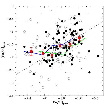
Figure 9.— The [Fe/H]_phot measurements are compared to the independently measured [Fe/H]_spec values, over a 1.5 dex spread in [Fe/H]_phot. The dashed line illustrates equality between the two measurements, and, in general, our data points follow this trend nicely for [Fe/H]_phot $>$ $-$2.2. The scatter among the spectroscopically measured abundances is large, as expected given the low $S/N$ of our spectra. This is illustrated by plotting the symbols as a function of the spectral $S/N$, where crosses represent all stars with a spectral $S/N$ $<$ 3, open circles represent stars with 3 $<$ $S/N$ $<$ 5, and filled circles represent stars with $S/N$ $>$ 5. The scatter in [Fe/H]_spec is clearly reduced among the better quality data. The larger data points with error bars are binned averages of the $S/N$ $>$ 3 data, where the photometric metallicities have been calculated using the Vandenberg, Bergbusch, & Dowler (2006) isochrones with an age of 12 Gyr and [$\alpha$/Fe] = 0.0. The two solid blue and green lines show the same comparison for different assumptions on age and [$\alpha$/Fe], as discussed in § 5.2.

We also illustrate how the independent photometric and spectroscopic metallicity measurements compare for various $S/N$ cuts. The crosses in Figure 9 illustrate those objects with $S/N$ $<$ 3, the open circles represent stars with 3 $<$ $S/N$ $<$ 5, and the filled points are those with $S/N$ $>$ 5. The higher $S/N$ points tend to be clustered closer to the 1:1 line as compared to the measurements from poorer quality spectra, indicating that much of the vertical scatter in the diagram results from poor characterization of the Ca ii triplet lines in these spectra.

Figure 10.— The discrete photometric metallicity distribution functions (MDF) for And I, II, and III (top) and the corresponding cumulative distributions (bottom), based on our confirmed sample of member stars in each dSph. The dashed line is held fixed at [Fe/H]_phot = $-$1.75 in each panel as a guide. We find that And III is the most metal-poor dSph of the three, and that And I is the most metal-rich. The metallicity dispersion in all three dSphs is similar, $\sigma_{\rm[Fe/H]}$ = 0.3 – 0.4.

To summarize, we find a nice overall agreement between our photometric and spectroscopic metallicity measurements for these satellites, indicating that any systematic biasses are likely small. For example, if we assume the dSphs are significantly younger than 12 Gyr, the resulting comparison of metallicities leads to a relation offset than the 1:1 line. We illustrate this, for an age of 6 Gyr, as the green curve in Figure 9. We also investigate the effects of different $\alpha$-enhancements. The photometric metallicities shown in Figure 9 assume these three dSphs are not enhanced in $\alpha$-elements relative to the Sun (e.g., we used the isochrones with [$\alpha$/Fe] = 0.0 for these calculations). Stars in the Milky Way’s field halo, and globular clusters, are known to be $\alpha$-enhanced ([$\alpha$/Fe] = $+$0.3) and it is generally believed that this is a result of the stars in the halos of galaxies forming in early “bursts”. Milky Way dSphs also show some $\alpha$-enhancement, although not as high as that measured in globular clusters. For example, Shetrone, Cote, & Sargent (2001) find $+$0.02 $<$ [$\alpha$/Fe] $<$ $+$0.13 for the three dSphs Draco, Sextans, and Ursa Minor. A mild $\alpha$-enhancement, such as that seen in these Milky Way galaxies, produces a very small affect on our metallicity measurements. However, we note that if And I, II, and III are enhanced in $\alpha$-elements at a level similar to Galactic globular clusters (e.g., [$\alpha$/Fe] = $+$0.3), then our overall photometric metallicities would become more metal-poor by $\sim$0.1 – 0.2 dex. This comparison is shown as a blue curve in Figure 9.

Our two independent metallicity measurements generally agree with one another, and we have shown that the scatter in the spectroscopic metallicities results largely from poor $S/N$. Therefore, we will adopt the photometric metallicities for the subsequent analysis. We stress that the reported abundances are derived from a secure sample of member stars in each satellite.

5.3. Abundance Distributions

The photometric metallicity distribution functions (MDFs) for the confirmed RGB stars in each of And I, II, and III in displayed in Figure 10. The top panels show discrete histograms and the bottom panels show the cumulative distributions. The dashed line marks a fixed guide at [Fe/H] = $-$1.75 in both panels. As was apparent from the CMDs, we confirm that all three of these dSphs are in fact metal-poor galaxies, with And I being slightly more metal-rich relative to And II and III. We find that the internal abundance spread of all three galaxies is quite similar, differing by less than 0.1 dex. Formally, we measure the mean metallicity, error in the mean, and dispersion to be [Fe/H]_phot = $-$1.45 $\pm$ 0.04 ($\sigma_{\rm[Fe/H]}$ = 0.37) for And I, [Fe/H]_phot = $-$1.64 $\pm$ 0.04 ($\sigma_{\rm[Fe/H]}$ = 0.34) for And II, and [Fe/H]_phot = $-$1.78 $\pm$ 0.04 ($\sigma_{\rm[Fe/H]}$ = 0.27) for And III.

Abundance analysis of And VII, X, and XIV were presented in Grebel & Guhathakurta (1999), Kalirai et al. (2009), and Majewski et al. (2007). Summarizing, the high resolution spectroscopic data for And VII in Guhathakurta, Reitzel, & Grebel (2000) did not yield an abundance measurement due to the low $S/N$ of the 18 confirmed giants at the Ca ii triplet. Therefore, we adopt And VII’s metallicity from the Keck/LRIS photometric study of Grebel & Guhathakurta (1999), who find [Fe/H]_phot = $-$1.4 $\pm$ 0.3 (the dispersion in metallicity was not measured). For And X, Kalirai et al. (2009) measured both a spectroscopic and photometric metallicity and found these to be in nice agreement. They find that And X is a metal-poor galaxy with [Fe/H]_phot = $-$1.93 $\pm$ 0.11, and exhibits a large metallicity dispersion of $\sigma_{\rm[Fe/H]}$ = 0.48. For a distance modulus of 24.7, the the photometric metallicity of And XIV is very low, [Fe/H] = $-$2.26 $\pm$ 0.05 (there is no metallicity dispersion measurement). These results are also summarized in Table 2.

For And I, II, and III, we can compare our metallicity results to the Da Costa et al. (1996; 2000; 2002) HST/WFPC2 study. Da Costa et al. transformed their photometry from the native HST filters to Johnson-Cousins, and then compared the color of the RGB stars to a set of giant branches for Galactic globular clusters (i.e., alpha-enhanced populations). As we noted earlier, their study of And I is likely affected by the metal-rich stream debris that we eliminated from this sightline in § 3. Interestingly, our mean metallicity is still identical to what they found, [Fe/H]_phot = $-$1.45 $\pm$ 0.20, suggesting that their value was in fact underestimated. As expected, our dispersion is much smaller than their study, $\sigma_{\rm[Fe/H]}$ = 0.60. Our sample only includes stars with [Fe/H] $<$ $-$0.92 given the detected substructure in this field, and, therefore, we would have eliminated the presence of any metal-rich tail in this dSph. For And II, we find a very similar abundance spread in the galaxy compared to the results of Da Costa et al. ($\sigma_{\rm[Fe/H]}$ = 0.36), however our mean metallicity is more metal-poor than their study by $\sim$0.15 dex. For And III, our mean metallicity is consistent with the Da Costa et al. study within their larger error bar ([Fe/H]_phot = $-1.88\pm 0.11$), however our internal metallicity dispersion is more than 2$\times$ larger than their measurement ($\sigma$ = 0.12).

Recently, McConnachie, Arimoto, & Irwin (2007) imaged And II using the wide-field Subaru Suprime-Cam instrument to a photometric depth below the horizontal branch. Their analysis suggests that the dSph contains two distinct components. For the dominant extended component, they find an old population with [Fe/H] = $-$1.5 and $\sigma_{\rm[Fe/H]}$ = 0.28. For the more concentrated inner region of the dSph, they find an intermediate aged (7 – 10 Gyr) and metal-rich ([Fe/H] = $-$1.2 and $\sigma_{\rm[Fe/H]}$ = 0.40) population. Confirming this picture with our present spectroscopic data is difficult given the limited spatial coverage (e.g., lack of many stars near the center of the galaxy), however, we have now obtained five times as many spectroscopic measurements over the face of this galaxy. These data, consisting of $\sim$500 individual radial velocity measurements of And II members, will present a much cleaner view of the nature of And II’s stellar populations.

Overall, our results suggest that the chemical abundances and abundance spread (where available) of the brighter four M31 satellites in our sample are quite similar, and that there is no evidence suggesting the evolutionary histories of these galaxies were significantly different. The two faintest satellites in this clean sample, And X and XIV, are found to be more metal-poor than the brighter satellites. Of course, a full analysis will require deeper photometric observations of the main-sequence turnoff morphology in each system, from which a full star formation history can be derived in conjunction with these metallicity measurements. We also note that the metallicities of the M31 halo dSphs is similar to the mean metallicity of M31’s stellar halo, determined by Kalirai et al. (2006a) and Chapman et al. (2006) to be [Fe/H] $\sim$ $-$1.5.

6. Global Properties:
Comparing Milky Way and M31 dSphs

6.1. An Inventory of the Milky Way and M31 dSphs

As we introduced earlier, wide field imaging surveys have recently uncovered many new dSph galaxies orbiting the Milky Way. As rapidly as these systems are being discovered, different groups have targeted individual giant and dwarf stars with multiobject spectrographs to characterize the radial velocities, velocity dispersions, and spectroscopic abundances of these systems. For comparison to our M31 sample, we begin by considering only those Milky Way dSphs in which the intrinsic velocity dispersion has been resolved.

Our baseline catalogue of properties for the classical Milky Way dSphs is drawn from Irwin & Hatzidimitriou (1995) and the review by Mateo (1998), updated to reflect recent photometric and spectroscopic analysis on a galaxy by galaxy basis where available. Our sample includes the Milky Way dSphs Carina, Draco, Fornax, Leo I, Leo II, Sculptor, Sextans, and Ursa Minor, as well as the more distant Local Group dSphs Tucana and Cetus (McConnachie & Irwin, 2006; Lewis et al., 2007). For the core radii and central velocity dispersions, we adopt values from Wolf et al. (2009) who present a summary of the most updated results in their Table 1 (see full references in their study, including Walker, Mateo, & Olszewski 2009). The [Fe/H] of most of these galaxies is updated from the Mateo (1998) results based on new multiobject studies of larger numbers of stars. For example, for Carina, Fornax, Sculptor, and Sextans we use the latest DART team results (Helmi et al., 2006), for Leo I and Leo II we use the Koch et al. (2007a) and Koch et al. (2007b) studies, and for Draco and Ursa Minor we adopt the values in Winnick (2003). If it is not directly measured in these studies, we have assumed an uncertainty of 10% in the half light radius of each galaxy. For the newly discovered lower luminosity Milky Way dSphs, our sample includes Bootes I, Bootes II, Canes Venatici I, Canes Venatici II, Coma Berenices, Hercules, Leo IV, Leo T, Segue I, Ursa Major I, and Ursa Major II. The baseline properties, such as luminosity and half-light radius, come from the summary table in Wolf et al. (2009) (see references therein and also the structural analysis in Martin, de Jong, & Rix 2008), velocity dispersions come from the Keck/DEIMOS spectroscopic study by Simon & Geha (2007), and abundances come from Kirby et al. (2008). The core radii of the dSphs is again taken from the King model fits in Strigari et al. (2008b), with a 10% assumed error. We note that the core radius of Bootes I is not known and so we have made an approximation such that $r_{c}$ $\sim$ $R_{e}$. This can lead to a $\sim$25% uncertainty (Martin et al., 2007), which has been factored into the calculation of dynamical masses (see below).

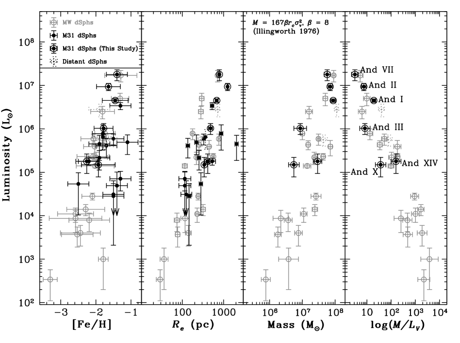
Figure 11.— The properties of M31 dSphs are compared to Milky Way dSphs of the same luminosity (see § 6 for references). The Milky Way dSphs are illustrated with as grey points whereas the M31 points are darker. The six M31 galaxies for which we have resolved intrinsic velocity dispersion measurements from the present study are dark encircled points. Finally, the three distant Local Group dSphs, Cetus, Tucana, and And XVIII are shown with dotted points and errorbars. All results are summarized in Table 3. The left panel illustrates the luminosity-metallicity relation, where we find excellent overlap between the M31 and Milky Way satellites, suggesting these systems have had similar chemical evolution histories. Four of the faintest M31 dSphs are found to be signicantly more metal-rich than expected from the trend, and therefore may be systems that have experienced tidal stripping (i.e., they are underluminous for their metallicity). The error bars in this plot represent the dispersion in metallicity in each galaxy. For several dSphs lacking such measurements (mostly in M31), the dispersion has been arbitrarily set to 0.30 dex (see Table 3). The middle-left panel illustrates the luminosity-size relation, where the size is represented by the 2D elliptical half-light radius. Although the brightest M31 satellites are larger than Milky Way dSphs of the same luminosity (see also McConnachie & Irwin 2006), we find that lower luminosity systems have similar sizes and therefore dynamical effects are unlikely to have truncated the sizes of these systems in a systematic way. The masses and mass-to-light ratios of the M31 dSphs, as calculated using the simplified technique described in § 4, are illustrated in the two right panels. The overall trend of decreasing total mass-to-light ratio with increasing luminosity is similar for the dSphs of each galaxy, although two of the faintest M31 dSphs in our sample appear to be less massive than their Milky Way counterparts. Combined with their similar (or larger) sizes, there is mild evidence that the densities of these galaxies are lower. This is verified by considering the more carefully calculated mass at the half light radius based on the new Wolf et al. (2009) method, as described in § 6.4 and presented in Figure 13.

For the 19 M31 dSphs, plus And XVIII which appears to be a background object, we adopt parameters primarily from the discovery papers summarized earlier as well as the analysis of McConnachie & Irwin (2006) for the brightest satellites. The half light radii in McConnachie & Irwin (2006) are computed as geometric means, and so we have adjusted these to an elliptical half-light radius ($R_{e}$) by factoring in the measured ellipticity. The metallicity of And V is taken from Armandroff, Davies, & Jacoby (1998) and for And VI and VII is taken from Grebel & Guhathakurta (1999). For the six satellites we’ve discussed in this paper, we adopt our new results based on the spectroscopically clean samples of stars. Again, a 10% error in the core radius is assumed (i.e., for the calculation of dynamical masses) if it has not been measured in the earlier papers. As discussed in § 1, the limited kinematic data presented for And IX and And XII (Chapman et al., 2005, 2007; Collins et al., 2009), And XI and XIII (Collins et al., 2009), and And XV and XVI (Letarte et al., 2009) have large uncertainties and are inconclusive in yielding accurate dynamical masses, and so we ignore them in the present analysis.

We recalculate the dynamical mass of each of the Milky Way dSphs summarized above using the same (simplified) technique described in § 4, with updated velocity dispersion and core radius measurements from these studies. More accurate masses of these Milky Way satellites at the half light radii are calculated in Wolf et al. (2009). A summary of all of these current properties, for both the Milky Way dSphs with internal velocity dispersion measurements, and for all of the M31 dSphs, is given in Table 3.

6.2. Chemical Abundance Trends

Table 3 illustrates that the Milky Way and M31 each host $\sim$20 dSphs, and the bulk of these satellites have measured abundances and half light radii. The intrinsic luminosity range of the M31 dSphs is of course smaller than the Milky Way satellites, however the two distributions overlap over a factor of 1000 in luminosity. There exists a known luminosity-metallicity relation for Local Group dSphs extending down to the faintest systems (e.g., Mateo 1998; Grebel et al. 2003; Kirby et al. 2008), and the M31 satellites are found to track the brighter part of this relation remarkably well, e.g., from $L$ $\sim$ 10⁵ to 10⁷ $L_{\odot}$. We illustrate this in the left panel of Figure 11, where the darker encircled symbols represent the spectroscopically cleaned measurements from our present study. Such a strong correlation demonstrates that the gross chemical evolution histories of these satellites are similar, and, if at all, similarly affected by dynamical interactions from their different host environments (see § 6.5). As summarized in Table 3, the intrinsic metallicity spreads of the brightest satellites in the Milky Way and M31 are also similar to one another, and as large as 0.3 – 0.5 dex (the metallicity dispersion is indicated with horizontal error bars in Figure 11). These similarities indicate that the stars in these galaxies may have resulted from an extended (early) star formation history, with the earlier generation of stars polluting the interstellar medium for subsequent star formation bursts. Yet, the trends of these overall processes must be very similar in the dSphs of the two hosts, and therefore minimally affected by external influences. As we note below, the gravitational potential of the dSphs in the two hosts also appears to be similar. Neither of these two findings, that there is a correlation between luminosity and metallicity or that the intrinsic abundance spreads are large, are true for globular clusters (Harris, 1996).

Interestingly, four of the least luminous M31 dSphs (And XI, XII, XIII, and XX) are found to be significantly more metal-rich than expected given their luminosities. These four systems, with $-$7.3 $<$ $M_{\rm V}$ $<$ $-$6.3, are found to be 0.5 – 1 dex more metal-rich than a reasonable extrapolation of both the M31 population and from the Milky Way dSphs with similar luminosity. One possible interpretation of this trend is that these satellites were initially much more massive than present, and have subsequently experienced tidal stripping. Such a scenario could possibly preserve the mean metallicity of the galaxies, while at the same time, reduce their luminosities significantly. The presence of a positive radial abundance gradient (which is not known) towards the center of any of these dSphs would enhance this effect, as the more metal-poor stars in the outskirts would be preferentially stripped away (e.g., Chou et al. 2007). Unfortunately, testing the tidal stripping possibility requires detailed kinematic data for many stars in these satellites, especially at larger radii. Such a data set does not yet exist in these low-luminosity systems. Similar to the M31 sample, the faint Milky Way satellite Bootes II also deviates from the general trend, possibly suggesting a similar evolutionary history as outlined for these M31 satellites.

6.3. Physical Sizes

McConnachie & Irwin (2006) found the very interesting result that the sizes of M31’s dSphs appear to be a factor of two larger than Milky Way dSphs of similar luminosity. The sample in their photometric study included some of M31’s brightest satellites, And I, II, III, V, VI, and VII (e.g., down to $M_{\rm V}$ = $-$9.6). In Figure 11 (middle-left panel), we extend this comparison by a factor of 20 down to a luminosity of $M_{\rm V}$ = $-$6.3 by including all 19 M31 dSphs from the discovery papers summarized earlier. With the exception of the two newly found galaxies And XIX ($R_{e}$ = 2.07 kpc – corrected from a geometric mean to an elliptical radius; McConnachie et al. 2008), and And XXI ($R_{e}$ = 875 pc; Martin et al. 2009), the bulk of the newly found dSphs in M31 have sizes comparable to Milky Way counterparts of similar luminosity. We also note that the two outliers in the new data are all among the furthest galaxies along the line of sight, and have similar (or lower) luminosities than counterparts with smaller sizes. Therefore, the measurement of their sizes is more difficult given the fewer number of detected member stars.

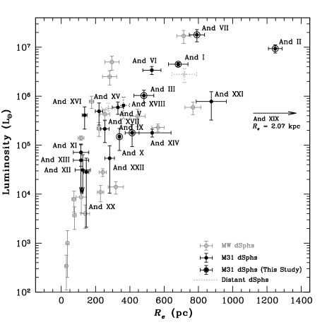
Figure 12.— The 2D elliptical half-light radii of Milky Way dSphs is compared to the M31 dSphs on a linear scale. In cases where the uncertainties in the half light radii were not directly measured, we have assumed it to be 10% in this plot. The general trend of dSphs in the two large hosts indicates that the most luminous M31 satellites extend to larger sizes than the Milky Way dSphs (see also McConnachie & Irwin 2006). However, for the bulk of the lower luminosity systems (e.g., $L$ $\lesssim$ 10⁶ $L_{\odot}$), the two distributions significantly overlap.

The overall size distribution of the two satellite systems can be better seen on an expanded linear scale, as presented in Figure 12. The distributions are found to significantly overlap between $L$ = 10⁴ and 10⁶ $L_{\odot}$. In fact, at lower luminosities, it appears And XI, XII, XIII, and XX all have systematically smaller half light radii than similar luminosity Milky Way galaxies such as Bootes I, Hercules, Leo T, and Ursa Major I. We note that the uncertainty in $R_{e}$ in both of these figures is arbitrarily taken to be 10% in cases where the error has not been directly measured. From this overall comparison, we can say that less than one-third of the M31 satellites are consistently larger than Milky Way counterparts of the same luminosity, and that this result is mostly limited to the brighter galaxies. This evidence therefore does not strongly support the claim that the Milky Way has a stronger tidal field that truncates its dSphs at a smaller radius relative to M31, unless such a dynamical effect could be limited to the brightest satellites.

6.4. Dark Matter Masses

The radial velocities from the SPLASH Survey presented in this paper allow us to measure dynamical masses for roughly one-third of the entire known population of M31’s dSphs. In Table 3, we have summarized the masses and mass-to-light ratios of these galaxies, based on the analysis presented in § 4 (i.e., using the Illingworth 1976 method). We have also recalculated the masses of the Milky Way dSphs with resolved central velocity dispersions using the same technique.

As we noted earlier, these mass measurements follow from a simple scaling relation involving the measured sizes and velocity dispersions of these galaxies, and assume an isotropic sphere in which mass follows light. Depending on the quality of the observations, several Milky Way dSphs allow modeling of the individual velocities to constrain the overall mass profile of the satellites (see e.g., Strigari et al. 2008b and Walker et al. 2009). Wolf et al. (2009) have presented a new prescription to calculate the masses of such systems out to the half light radius, and show that these results agree well with with full dynamical modeling approach. We summarize the masses calculated from this technique, both for Milky Way and M31 satellites, in the last column of Table 3. As Wolf et al. (2009) show, the Illingworth (1976) approximation systematically underpredicts the mass of dSphs and so the new $M_{1/2}$ are often similar, if not larger, than those values. This newer analysis is discussed in more detail below.

In the two right panels of Figure 11, we illustrate the total measured masses and mass-to-light ratios of Milky Way dSphs and the six M31 dSphs that are the focus of this paper. Overall, the trend of increasing total mass of Milky Way dSphs with higher luminosity persists in the M31 dSphs. The slope of the relation between the two families of dSphs is also very similar. At the luminous end, our sample includes the two brightest M31 dSphs known, And II and VII, both of which have a similar luminosity to the Galactic dSph Fornax. Formally, our measurements indicate that the total masses of these three dSphs is 6 – 9 $\times$ 10⁷ $M_{\odot}$. At slightly lower luminosities, we find that the $M/L_{\rm V}$ of And I ($M_{\rm V}$ = $-$11.8) is higher by a factor of two compared to the Milky Way dSph Leo I ($M_{\rm V}$ = $-$11.5), yet is lower by a factor of two compared to the luminous distant Local Group dSph Cetus ($M_{\rm V}$ = $-$11.3). For our three fainter satellites, we find that the $M/L_{\rm V}$ of And XIV is in nice agreement with the comparable Milky Way dSphs Draco, Canes Venatici I, and Leo T. However, for And III and And X, we find that the measured $M/L_{\rm V}$ is smaller by several factors compared to most Milky Way dSphs of comparable brightness, such as Draco, Sextans, Ursa Minor, Canes Venatici I, and Leo T, and therefore these galaxies contain less dark matter than their Milky Way counterparts (see also Kalirai et al. 2009).

For the luminous dSphs, the comparisons above demonstrate that, despite having a larger size than their Milky Way counterparts of the same luminosity, the masses of dSphs around each of the two hosts are similar. At lower luminosities, we see mild evidence that two of the six M31 satellites in our sample have a lower mass than their Milky Way counterparts. As these latter two satellites have half light radii that are similar, if not slightly larger, than Milky Way dSphs, this hints at an overall trend of the six M31 dSphs being less dense than Milky Way dSphs.

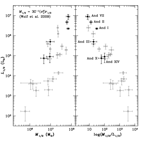
Figure 13.— The masses (left) and mass-to-light ratios (right) of M31 (black) and Milky Way (grey) dSphs at the half light radius, calculated as described in Wolf et al. (2009). The comparison of dSphs in the two hosts indicates that the lower luminosity M31 dSphs have dynamical masses and mass-to-light ratios that track the lower mass edge of the general relation for Milky Way satellites. Although the dynamical masses of these satellites are generally smaller than their Milky Way counterparts, they have half light radii that are similar or larger (see Figures 11 and 12). These galaxies are therefore less dense than the Milky Way dSphs.

Strigari et al. (2008b) have recently constructed mass profiles for the Milky Way dSph population and surprisingly found that, over four orders of magnitude in luminosity, all of the satellites have approximately the same dark matter mass ($\sim$10⁷ $M_{\odot}$) within their central 300 pc. The interpretation of a common mass scale for Milky Way dSphs is still unclear, as discussed by Strigari et al. (2008b). For example, the common mass measurements may be indicative of a fundamental scale for dark matter clustering. Correctly measuring whether such a scale extends to M31’s dSphs, and if the absolute value is the same, will require both larger data sets (e.g., $\gtrsim$50 accurate radial velocities per dSph) and more sophisticated modeling techniques. In the last column of Table 3, we have calculated the masses of each of the M31 dSphs and Milky Way satellites at the half light radius ($M_{1/2}$), using the new Wolf et al. (2009) technique (see § 4.1). A comparison of $M_{1/2}$ between the Milky Way and M31 dSphs, at the same luminosity, verifies the findings above. At the luminous end of the distribution, the $M_{1/2}$ are similar despite the M31 dSphs being larger, while at lower luminosities, the $M_{1/2}$ are smaller for the M31 dSphs (e.g., And III, X, and XIV; see Figure 13). We will present the first results on the mass profiles of these M31 dSphs, and therefore the mass within a fixed physical radius, in Wolf et al. (2010, in prep.).

6.5. The Bigger Picture: The Milky Way vs M31

Although the Milky Way and M31 are both generally characterized as large spiral galaxies, several differences between the two systems have been pointed out in recent studies such as the SPLASH Survey. For example, surface brightness and abundance studies have shown that the metal-poor, stellar halo of M31 dominates the metal-rich inner spheroid at a radius of 20 – 30 kpc, much farther out than the transition point in the Milky Way (Guhathakurta et al., 2005; Irwin et al., 2005; Kalirai et al., 2006a; Chapman et al., 2006; Ibata et al., 2007; Koch et al., 2008). Additionally, the overall density of M31 at 20 kpc is much higher than the Milky Way (Reitzel, Guhathakurta, & Gould, 1998), and M31 contains a higher fraction of intermediate age stars than the Milky Way at these radii (Brown et al., 2007). Major differences among the population of satellites in the two systems have also long been known. The most luminous Milky Way satellites, the Small and Large Magellanic Clouds, are irregular type galaxies, of which M31 has none. The most luminous M31 satellites are the dwarf ellipticals NGC 205, NGC 187, and NGC 147, of which the Milky Way has none. The overall population of globular clusters in M31 outnumbers the Milky Way by several times.

The differences between the Milky Way and M31 are likely tied to their past accretion histories. Deep, wide field imaging surveys of M31 demonstrate a large amount of substructure both in the inner and outer halo (Ferguson et al., 2002; Ibata et al., 2007; McConnachie et al., 2009). Simulations of galaxy formation in the $\Lambda$CDM paradigm suggest that the inner halos of massive galaxies are built up quickly, and formed from just a few of the most massive, early accretion events (e.g., Diemand, Kuhlen, & Madau 2007). If the accretion history is responsible for the present day differences between the two large galaxies (e.g., M31 having experienced more interactions – Hammer et al. 2007), then it may be the case that the surviving satellites suffered enhanced stripping. As we have discussed, the overall sizes of the M31 dSphs are systematically larger than their Milky Way counterparts at the luminous end (see also McConnachie & Irwin 2006), and the dynamical masses of M31’s dSphs are either similar or lower than comparable luminosity Milky Way dSphs. However, in order to “puff” these systems up into less dense objects, the interactions would have had to strip the dark matter halos within the visible radii of the galaxies, in which case the stars should also be stripped.

An alternate mechanism for losing stars through stripping has also just been presented by D’Onghia et al. (2009). They simulate the interactions of dwarf disk galaxies with larger systems and find that the encounters can excite gravitational resonances. They refer to this process as “resonant stripping” and show that the dwarf disk galaxies can transform to systems that look like present day dSphs (gas poor, dark matter dominated). Resonant stripping allows for up to 80% of the deeply embedded stellar component in satellite galaxies to be lost after a few Gyrs of interaction, while, at the same time, much less strongly affecting the surrounding dark matter halos. Therefore the mass-to-light ratios of these galaxies, and the sizes of their stellar distribution, can be altered depending on the details of the interaction history (e.g., prograde vs retrograde orbits and the degree and timescale of the encounters). Unfortunately, such an effect is difficult, if not impossible, to measure from the limited angular spread of our radial velocities, which are not well extended in large numbers to the tidal radius of each satellite. A thorough investigation of the tidal interaction of these satellites with M31, and specifically relating such interactions to those of similar luminosity Milky Way dSphs, will also require an understanding of the orbits of these galaxies. Tangential velocities are currently only available for a few of the most luminous Milky Way satellites, and for none of the M31 dSphs.

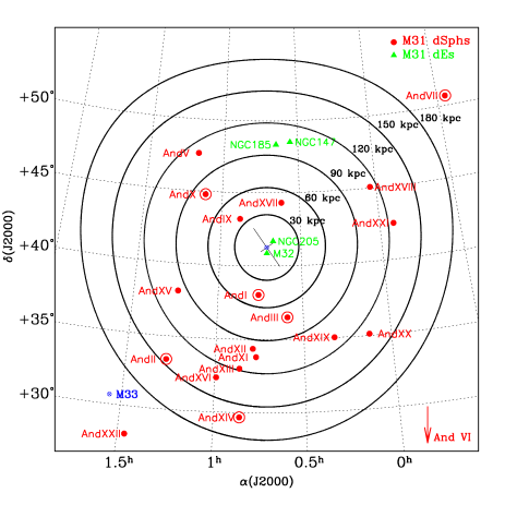
Figure 14.— The location of M31’s 18 dSphs relative to the center of the galaxy is shown as filled red circles. The six dSphs comprising this study are also indicated with larger open circles, and clearly span a wide range in distance from M31 and azimuth. As described in the text, the bias of satellites in the south results from incomleteness in the imaging surveys.

To first order, we can investigate the projected distribution of M31’s 19 dSphs relative to the center of the galaxy, as shown in Figure 14. The dSph distribution spans over 30 degrees in right ascension and declination on this Figure (red circles). The concentric annuli are each separated by 30 kpc, and extend outward to 180 kpc from M31. The small lines at the center of the figure mark the size of M31’s optical disk. Also shown are the locations of M33, and M31’s 4 dwarf ellipticals (green triangles). First, this figure demonstrates that there is a clear absence of M31 satellites in the northern regions of the galaxy. The cause of this is an observational bias related to the location of deep imaging surveys that have thus far only explored more southern latitudes (e.g., Ibata et al. 2007 and McConnachie et al. 2009). These surveys, e.g., PAandAS, are only now beginning to target other areas of the galaxy, and will surely uncover additional dSphs in M31, as will Pan-STARRS (Kaiser et al. 2002). The four recent discoveries of And XVIII, And XIX, And XX, and And XXI in the western hemisphere of M31 reflect the extention of the initial CFHT MegaCam survey (McConnachie et al., 2008; Martin et al., 2009).

The six satellites in our study are shown with enclosed open circles in Figure 14. These dSphs span an appreciable range in radius and azimuth relative to M31. And I, III, and X sample intermediate radii in the halo, from $R$ = 45 – 75 kpc, whereas And II, VII, and XIV are all located in the outskirts of M31’s stellar halo, $R\gtrsim$ 150 kpc. In this context, one or more of the three inner satellites may represent close-in bodies that were captured long ago, whereas the outer group could be, in part, dSphs that are just now starting to fall into M31’s potential. Evidence of such falling in galaxies is also supported by the radial velocity of And XIV as discussed earlier (see also Majewski et al. 2007), and also in the case of And XII (Chapman et al., 2007). However, both sets of galaxies, near and far from M31’s center, include satellites that are systematically larger than Milky Way dSphs, as we showed in Figure 11.

Interestingly, the three lower luminosity M31 satellites And XI, XII, and XIII appear to be smaller than a Milky Way counterpart of similar luminosity (Bootes I), and are also located in a similar projected position in M31. Kinematics of these galaxies will reveal if they are in fact moving at similar radial velocities, possibly suggesting an infalling group (e.g., see Li & Helmi 2008; D’Onghia 2008). The dark matter masses of these satellites, in relation to the general trend of Milky Way vs M31 dSphs, will help gauge the degree to which external dynamical influences may have played a role in shaping the internal kinematics. More generally, the future of resolved spectroscopy of M31 dSphs is sure to shed light on both the intrinsic properties of the satellites and on the galaxy formation and evolution processes that shape these properties.

7. Conclusions

We present the first systematic large scale spectroscopic survey of M31’s dSphs as a part of the SPLASH Survey, a detailed study of And I, II, III, VII, X, and XIV. The fundamental properties of these galaxies are established from a sample of confirmed member stars, including the mean radial velocity, velocity dispersion, mean abundance, abundance spread, and total (stellar + dark matter) mass. The kinematics indicate that the radial velocity and intrinsic velocity dispersion of the six satellites are $v_{\rm rad}=-375.8\pm 1.4$ km s^-1 and $\sigma_{v}=10.6\pm 1.1$ km s^-1 for And I, $v_{\rm rad}=-193.6\pm 1.0$ km s^-1 and $\sigma_{v}=7.3\pm 0.8$ km s^-1 for And II, $v_{\rm rad}=-345.6\pm 1.8$ km s^-1 and $\sigma_{v}=4.7\pm 1.8$ km s^-1 for And III, $v_{\rm rad}=-309.4\pm 2.3$ km s^-1 and $\sigma_{v}=9.7\pm 1.6$ km s^-1 for And VII, $v_{\rm rad}=-168.3\pm 1.2$ km s^-1 and $\sigma_{v}=3.9\pm 1.2$ km s^-1 for And X, and $v_{\rm rad}=-481.0\pm 1.2$ km s^-1 and $\sigma_{v}=5.4\pm 1.3$ km s^-1 for And XIV.

Both photometric and spectroscopic metallicities are measured for all confirmed member stars in each galaxy, and the two independent measurements agree nicely with one another. We find that the six dSphs are metal-poor systems with a mean iron abundance of [Fe/H]_phot = $-1.45\pm 0.04$ ($\sigma_{\rm[Fe/H]}$ = 0.37) for And I, [Fe/H]_phot = $-1.64\pm 0.04$ ($\sigma_{\rm[Fe/H]}$ = 0.34) for And II, [Fe/H]_phot = $-1.78\pm 0.04$ ($\sigma_{\rm[Fe/H]}$ = 0.27) for And III, [Fe/H]_phot = $-1.40\pm 0.30$ for And VII, [Fe/H]_phot = $-1.93\pm 0.11$ ($\sigma_{\rm[Fe/H]}$ = 0.248) for And X, and [Fe/H]_phot = $-2.26\pm 0.05$ for And XIV (where two of the satellites lack a metallicity dispersion measurement).

The dynamical mass of each satellite is estimated to first order using the Illingworth (1976) formalism. More accurate mass measurements at the half-light radius of each galaxy are also calculated using the methods described in Wolf et al. (2009). As summarized in Table 2 and 3, these yield half-light radius mass-to-light ratios of $M_{1/2}$/$L_{1/2}$ = 31 $\pm$ 6 for And I, 13 $\pm$ 3 for And II, 19 $\pm$ 12 for And III, 7.7 $\pm$ 2.8 for And VII, 63 $\pm$ 40 for And X, and 102 $\pm$ 71 for And XIV. These calculations are found to agree nicely with masses measured through full modeling of the individual radial velocities assuming the dark matter follows a five parameter density profile.

The comparison of the overall properties of M31’s dSphs with Milky Way dSphs of similar luminosity indicates some interesting similarities and differences. For example, we find that the luminosity – metallicity relation is very similar between $L$ $\sim$ 10⁵ – 10⁷ $L_{\odot}$, suggesting that the chemical evolution histories of each group of dSphs is similar. The lowest luminosity M31 dSphs appear to deviate from the relation, possibly suggesting tidal stripping. The previous finding of McConnachie & Irwin (2006) indicating that the brightest M31 dSphs are systematically larger than Milky Way counterparts of the same luminosity does not persist cleanly to lower luminosities. We find that the sizes of dSphs in the two hosts significantly overlap for $L$ = 10⁴ – 10⁶ $L_{\odot}$, and that four of the faintest M31 dSphs are smaller than Milky Way satellites of similar luminosity. The first dynamical mass measurement comparisons between the M31 and Milky Way dSphs hints that the M31 satellites are systematically less dense than Milky Way counterparts.

Table 3

Galaxy	$M_{\rm V}$	$L_{\rm V}$ ($L_{\odot}$)	$d$ (kpc)	$\sigma_{v}$ (km s-1)	$r_{c}$ (pc)	$R_{e}$ (pc)	$r_{1/2}$ (pc)	[Fe/H]	$\sigma_{[Fe/H]}$	$M$ ($M_{\odot}$)	$M$/$L$ ($M_{\odot}$/$L_{\odot}$)	$M_{1/2}$ ($M_{\odot}$)
M31 dSphs – This Study
And I	$-$11.8	(4.5 $\pm$ 0.4) $\times$ 106	745 $\pm$ 24	10.6 $\pm$ 1.1	580 $\pm$ 60	682 $\pm$ 57	900 $\pm$ 75	$-$1.45 $\pm$ 0.04	0.37	(8.7 $\pm$ 1.6) $\times$ 107	19 $\pm$ 4	(7.0 $\pm$ 1.2) $\times$ 107
And II	$-$12.6	(9.4 $\pm$ 1.8) $\times$ 106	652 $\pm$ 18	7.3 $\pm$ 0.8	990 $\pm$ 40	1248 $\pm$ 40	1659 $\pm$ 53	$-$1.64 $\pm$ 0.04	0.34	(7.0 $\pm$ 1.1) $\times$ 107	7.5 $\pm$ 1.8	(6.1 $\pm$ 1.0) $\times$ 107
And III	$-$10.2	(1.0 $\pm$ 0.3) $\times$ 106	749 $\pm$ 24	4.7 $\pm$ 1.8	290 $\pm$ 40	482 $\pm$ 58	638 $\pm$ 77	$-$1.78 $\pm$ 0.04	0.27	(8.6 $\pm$ 4.8) $\times$ 106	8.3 $\pm$ 5.2	(9.6 $\pm$ 5.4) $\times$ 106
And VII	$-$13.3	(1.8 $\pm$ 0.5) $\times$ 107	763 $\pm$ 35	9.7 $\pm$ 1.6	450 $\pm$ 20	791 $\pm$ 45	1050 $\pm$ 60	$-$1.4 $\pm$ 0.30	$\cdots$	(5.7 $\pm$ 1.3) $\times$ 107	3.2 $\pm$ 1.2	(6.9 $\pm$ 1.6) $\times$ 107
And X	$-$8.1	(1.5 $\pm$ 0.7) $\times$ 105	701 $\pm$ 37	3.9 $\pm$ 1.2	271 $\pm$ 27	339 $\pm$ 6	448 $\pm$ 8	$-$1.93 $\pm$ 0.11	0.48	(5.5 $\pm$ 2.5) $\times$ 106	37 $\pm$ 24	(4.7 $\pm$ 2.0) $\times$ 106
And XIV	$-$8.3	(1.8 $\pm$ 0.9) $\times$ 105	871 $\pm$ 87	5.4 $\pm$ 1.3	734 $\pm$ 73	413 $\pm$ 41	461 $\pm$ 155	$-$2.26 $\pm$ 0.05	0.31	(2.9 $\pm$ 1.0) $\times$ 107	160 $\pm$ 95	(9.2 $\pm$ 4.4) $\times$ 106
Other M31 dSphs
And V	$-$9.6	(5.9 $\pm$ 1.7) $\times$ 105	774 $\pm$ 28	$\cdots$	280 $\pm$ 40	330 $\pm$ 33	$\cdots$	$-$1.5  $\cdots$	$\cdots$	$\cdots$	$\cdots$	$\cdots$
And VI	$-$11.5	(3.4 $\pm$ 0.6) $\times$ 106	783 $\pm$ 25	$\cdots$	480 $\pm$ 60	528 $\pm$ 53	$\cdots$	$-$1.3 $\pm$ 0.30	$\cdots$	$\cdots$	$\cdots$	$\cdots$
And IX	$-$8.3	(1.8 $\pm$ 0.3) $\times$ 105	787 $\pm$ 157	$\cdots$	309 $\pm$ 31	530 $\pm$ 110	$\cdots$	$-$2.2  $\cdots$	$\cdots$	$\cdots$	$\cdots$	$\cdots$
And XI	$-$7.3	(7.1 $\pm$ 3.4) $\times$ 104	783 $\pm$ 78	$\cdots$	$\cdots$	115 $\pm$ 45	$\cdots$	$-$1.3  $\cdots$	$\cdots$	$\cdots$	$\cdots$	$\cdots$
And XII	$-$6.4	(3.1 $\pm$ 3.3) $\times$ 104	783 $\pm$ 78	$\cdots$	$\cdots$	125 $\pm$ 45	$\cdots$	$-$1.5  $\cdots$	$\cdots$	$\cdots$	$\cdots$	$\cdots$
And XIII	$-$6.9	(4.9 $\pm$ 5.2) $\times$ 104	783 $\pm$ 78	$\cdots$	$\cdots$	115 $\pm$ 45	$\cdots$	$-$1.4  $\cdots$	$\cdots$	$\cdots$	$\cdots$	$\cdots$
And XV	$-$9.4	(4.9 $\pm$ 2.4) $\times$ 105	630 $\pm$ 60	$\cdots$	167 $\pm$ 17	220 $\pm$ 22	$\cdots$	$-$1.1  $\cdots$	$\cdots$	$\cdots$	$\cdots$	$\cdots$
And XVI	$-$9.2	(4.1 $\pm$ 2.0) $\times$ 105	525 $\pm$ 50	$\cdots$	98 $\pm$ 10	136 $\pm$ 14	$\cdots$	$-$1.7  $\cdots$	$\cdots$	$\cdots$	$\cdots$	$\cdots$
And XVII	$-$8.5	(2.2 $\pm$ 1.0) $\times$ 105	794 $\pm$ 40	$\cdots$	$\cdots$	254 $\pm$ 25	$\cdots$	$-$1.9  $\cdots$	$\cdots$	$\cdots$	$\cdots$	$\cdots$
And XIX	$-$9.3	(4.5 $\pm$ 2.6) $\times$ 105	933 $\pm$ 61	$\cdots$	$\cdots$	2065 $\pm$ 206	$\cdots$	$-$1.9 $\pm$ 0.1	$\cdots$	$\cdots$	$\cdots$	$\cdots$
And XX	$-$6.3	(2.8 $\pm$ 2.6) $\times$ 104	802 $\pm$ 197	$\cdots$	$\cdots$	146 $\pm$ 15	$\cdots$	$-$1.5 $\pm$ 0.1	$\cdots$	$\cdots$	$\cdots$	$\cdots$
And XXI	$-$9.9	(7.8 $\pm$ 4.6) $\times$ 105	859 $\pm$ 51	$\cdots$	$\cdots$	875 $\pm$ 88	$\cdots$	$-$1.8  $\cdots$	$\cdots$	$\cdots$	$\cdots$	$\cdots$
And XXII	$-$7.0	(5.4 $\pm$ 4.4) $\times$ 104	1033 $\pm$ 103	$\cdots$	$\cdots$	282 $\pm$ 28	$\cdots$	$-$2.5  $\cdots$	$\cdots$	$\cdots$	$\cdots$	$\cdots$
Classical MW dSphs
Carina	$-$9.3	(4.3 $\pm$ 1.0) $\times$ 105	105 $\pm$ 2	6.4 $\pm$ 0.2	269 $\pm$ 37	254 $\pm$ 28	334 $\pm$ 37	$-$1.80 $\pm$ 0.02	0.30	(1.5 $\pm$ 0.2) $\times$ 107	34 $\pm$ 9	(9.6 $\pm$ 0.9) $\times$ 106
Draco	$-$8.6	(2.2 $\pm$ 0.7) $\times$ 105	76 $\pm$ 5	10.1 $\pm$ 0.5	169 $\pm$ 11	220 $\pm$ 11	291 $\pm$ 14	$-$1.99 $\pm$ 0.04	0.32	(2.3 $\pm$ 0.2) $\times$ 107	105 $\pm$ 35	(2.1 $\pm$ 0.3) $\times$ 107
Fornax	$-$13.3	(1.7 $\pm$ 0.5) $\times$ 107	147 $\pm$ 3	10.7 $\pm$ 0.2	586 $\pm$ 53	714 $\pm$ 40	944 $\pm$ 53	$-$1.29 $\pm$ 0.02	0.46	(9.0 $\pm$ 0.8) $\times$ 107	5.3 $\pm$ 1.6	(7.4 $\pm$ 0.4) $\times$ 107
Leo I	$-$11.9	(5.0 $\pm$ 1.6) $\times$ 106	254 $\pm$ 18	9.0 $\pm$ 0.4	459 $\pm$ 77	295 $\pm$ 49	388 $\pm$ 64	$-$1.31 $\pm$ 0.02	0.25	(5.0 $\pm$ 0.9) $\times$ 107	9.9 $\pm$ 3.6	(2.2 $\pm$ 0.2) $\times$ 107
Leo II	$-$9.9	(7.8 $\pm$ 2.2) $\times$ 105	233 $\pm$ 15	6.6 $\pm$ 0.5	179 $\pm$ 17	177 $\pm$ 13	233 $\pm$ 17	$-$1.74 $\pm$ 0.02	0.29	(1.0 $\pm$ 0.2) $\times$ 107	13 $\pm$ 4	(7.3 $\pm$ 1.1) $\times$ 106
Sculptor	$-$11.2	(2.5 $\pm$ 0.8) $\times$ 106	86 $\pm$ 5	9.0 $\pm$ 0.2	145 $\pm$ 41	282 $\pm$ 41	375 $\pm$ 54	$-$1.81 $\pm$ 0.02	0.34	(1.6 $\pm$ 0.5) $\times$ 107	6.3 $\pm$ 2.7	(2.3 $\pm$ 0.2) $\times$ 107
Sextans	$-$9.6	(5.9 $\pm$ 1.7) $\times$ 105	96 $\pm$ 3	7.1 $\pm$ 0.3	461 $\pm$ 35	768 $\pm$ 47	1019 $\pm$ 62	$-$2.07 $\pm$ 0.03	0.36	(3.1 $\pm$ 0.3) $\times$ 107	53 $\pm$ 16	(3.5 $\pm$ 0.5) $\times$ 107
Ursa Minor	$-$9.2	(3.9 $\pm$ 1.5) $\times$ 105	77 $\pm$ 4	11.5 $\pm$ 0.6	401 $\pm$ 51	445 $\pm$ 44	588 $\pm$ 58	$-$2.03 $\pm$ 0.04	0.32	(7.1 $\pm$ 1.0) $\times$ 107	182 $\pm$ 75	(5.6 $\pm$ 0.8) $\times$ 107
Lower Lum MW dSphs
Bootes I	$-$6.3	(2.8 $\pm$ 0.5) $\times$ 104	66 $\pm$ 3	9.0 $\pm$ 2.2	242 $\pm$ 61	242 $\pm$ 21	322 $\pm$ 28	$-$2.10 $\pm$ 0.30	$\cdots$	(2.6 $\pm$ 1.1) $\times$ 107	935 $\pm$ 433	(2.4 $\pm$ 1.5) $\times$ 107
Bootes II	$-$2.7	(1.0 $\pm$ 0.8) $\times$ 103	42 $\pm$ 8	10.5 $\pm$ 7.4	26 $\pm$ 3	36 $\pm$ 9	$\cdots$	$-$1.79 $\pm$ 0.05	0.14	(3.8 $\pm$ 3.8) $\times$ 106	3830 $\pm$ 4909	$\cdots$
Canes Venatici I	$-$8.6	(2.3 $\pm$ 0.4) $\times$ 105	218 $\pm$ 10	7.6 $\pm$ 0.5	554 $\pm$ 55	564 $\pm$ 36	750 $\pm$ 48	$-$2.08 $\pm$ 0.02	0.46	(4.3 $\pm$ 0.5) $\times$ 107	186 $\pm$ 41	(2.8 $\pm$ 0.7) $\times$ 107
Canes Venatici II	$-$4.9	(7.9 $\pm$ 3.7) $\times$ 103	160 $\pm$ 5	4.6 $\pm$ 1.0	132 $\pm$ 13	74 $\pm$ 12	97 $\pm$ 16	$-$2.19 $\pm$ 0.05	0.58	(3.7 $\pm$ 1.2) $\times$ 106	472 $\pm$ 264	(1.4 $\pm$ 0.8) $\times$ 106
Coma Berenices	$-$4.1	(3.7 $\pm$ 1.8) $\times$ 103	44 $\pm$ 4	4.6 $\pm$ 0.8	64 $\pm$ 6	77 $\pm$ 10	100 $\pm$ 13	$-$2.53 $\pm$ 0.05	0.45	(1.8 $\pm$ 0.5) $\times$ 106	489 $\pm$ 271	(2.0 $\pm$ 0.7) $\times$ 106
Hercules	$-$5.3	(1.1 $\pm$ 0.4) $\times$ 104	133 $\pm$ 6	5.1 $\pm$ 0.9	321 $\pm$ 32	229 $\pm$ 19	305 $\pm$ 26	$-$2.58 $\pm$ 0.04	0.51	(1.1 $\pm$ 0.3) $\times$ 107	1014 $\pm$ 459	(7.5 $\pm$ 4.4) $\times$ 106
Leo IV	$-$5.0	(8.7 $\pm$ 4.5) $\times$ 103	160 $\pm$ 15	3.3 $\pm$ 1.7	152 $\pm$ 15	116 $\pm$ 30	151 $\pm$ 39	$-$2.58 $\pm$ 0.08	0.75	(2.2 $\pm$ 1.6) $\times$ 106	254 $\pm$ 230	(1.1 $\pm$ 2.2) $\times$ 106
Leo T	$-$8.1	(1.4 $\pm$ 0.1) $\times$ 105	407 $\pm$ 38	7.8 $\pm$ 1.6	170 $\pm$ 17	115 $\pm$ 17	152 $\pm$ 21	$-$2.02 $\pm$ 0.05	0.54	(1.4 $\pm$ 0.4) $\times$ 107	99 $\pm$ 32	(7.4 $\pm$ 3.7) $\times$ 106
Segue I	$-$1.5	(3.4 $\pm$ 2.3) $\times$ 102	23 $\pm$ 2	4.3 $\pm$ 1.1	31 $\pm$ 3	29 $\pm$ 7	38 $\pm$ 9	$-$3.30 $\pm$ 0.20	$\cdots$	(7.7 $\pm$ 2.9) $\times$ 105	2252 $\pm$ 1742	(6.0 $\pm$ 3.9) $\times$ 105
Ursa Major I	$-$5.6	(1.4 $\pm$ 0.4) $\times$ 104	97 $\pm$ 4	7.6 $\pm$ 1.0	308 $\pm$ 31	318 $\pm$ 45	416 $\pm$ 58	$-$2.29 $\pm$ 0.04	0.54	(2.4 $\pm$ 0.5) $\times$ 107	1698 $\pm$ 603	(1.3 $\pm$ 0.6) $\times$ 107
Ursa Major II	$-$4.2	(4.0 $\pm$ 2.0) $\times$ 103	32 $\pm$ 4	6.7 $\pm$ 1.4	127 $\pm$ 13	140 $\pm$ 25	184 $\pm$ 33	$-$2.44 $\pm$ 0.06	0.57	(7.6 $\pm$ 2.4) $\times$ 106	1904 $\pm$ 1222	(7.9 $\pm$ 4.4) $\times$ 106
Distant LG dSphs
Cetus	$-$11.3	(2.8 $\pm$ 0.9) $\times$ 106	755 $\pm$ 23	17.0 $\pm$ 0.2	290 $\pm$ 29	718 $\pm$ 72	$\cdots$	$-$1.9  $\cdots$	$\cdots$	(1.1 $\pm$ 0.1) $\times$ 108	40 $\pm$ 14	$\cdots$
Tucana	$-$9.5	(5.6 $\pm$ 1.6) $\times$ 105	880 $\pm$ 40	15.8 $\pm$ 3.6	130 $\pm$ 13	274 $\pm$ 40	$\cdots$	$-$1.7 $\pm$ 0.2	0.30	(4.3 $\pm$ 1.5) $\times$ 107	77 $\pm$ 34	$\cdots$
And XVIII	$-$9.7	(6.5 $\pm$ 3.1) $\times$ 105	1355 $\pm$ 88	$\cdots$	$\cdots$	363 $\pm$ 36	$\cdots$	$-$1.8 $\pm$ 0.1	$\cdots$	$\cdots$	$\cdots$	$\cdots$

References

- Armandroff, Davies, & Jacoby (1998) Armandroff, T. E., Davies, J. E., & Jacoby, G. H. 1998, AJ, 116, 2287
- Belokurov et al. (2006) Belokurov, V., et al. 2006, ApJ, 647, L111
- Belokurov et al. (2007) Belokurov, V., et al. 2007, ApJ, 654, 897
- Belokurov et al. (2008) Belokurov, V., et al. 2008, ApJ, 686, L83
- Belokurov et al. (2009) Belokurov, V., et al. 2009, MNRAS, 397, 1748
- Brown et al. (2007) Brown, T., et al. 2007, ApJ, 658, L95
- Bullock, Kravtsov, & Weinberg (2000) Bullock, J. S., Kravtsov, A. V., & Weinberg, D. H. 2000, ApJ, 539, 517
- Bullock, Kravtsov, & Weinberg (2001) Bullock, J. S., Kravtsov, A. V., & Weinberg, D. H. 2001, ApJ, 548, 33
- Bullock & Johnston (2005) Bullock, J. S., & Johnston, K. V. 2005, ApJ, 635, 931
- Chapman et al. (2005) Chapman, S. C., Ibata, R. A., Lewis, G. F., Ferguson, A. M. N., Irwin, M., McConnachie, A. W., & Tanvir, N. 2005, ApJ, 632, L87
- Chapman et al. (2006) Chapman, S. C, Ibata, R., Lewis, G. F., Ferguson, A. M. N., Irwin, M., McConnachie, A., & Tanvir, N. 2006, ApJ, 653, 255
- Chapman et al. (2007) Chapman, S., et al. 2007, ApJ, 662, L79
- Chou et al. (2007) Chou, M.-Y., et al. 2007, ApJ, 670, 346
- Collins et al. (2009) Collins, M. L. M., et al. 2009, MNRAS submitted, arXiv:0911.1365
- Cote, Oke, & Cohen (1999) Cote, P., Oke, J. B., & Cohen, J. G. 1999, AJ, 118, 1645
- Cote et al. (1999) Cote, P., Mateo, M., Olszewski, E. W., & Cook, K. H. 1999, ApJ, 526, 147
- D’Onghia (2008) D’Onghia, E. 2008, ApJ, submitted, arXiv:0802.0302
- D’Onghia et al. (2009) D’Onghia, E., Besla, G., Cox, T. J., & Hernquist, L. 2009, Nature, 460, 7255
- Da Costa et al. (1996) Da Costa, G. S., Armandroff, T. E., Caldwell, N., & Seitzer, P. 1996, AJ, 112, 2576
- Da Costa et al. (2000) Da Costa, G. S., Armandroff, T. E., Caldwell, N., & Seitzer, P. 2000, AJ, 119, 705
- Da Costa, Armandroff, & Caldwell (2002) Da Costa, G. S., Armandroff, T. E., Caldwell, N. 2002, AJ, 124, 332
- Demarque et al. (2004) Demarque, P., Woo, J.-H., Kim, Y.-C., & Yi, S. K. 2004, ApJS, 155, 667
- Diemand, Kuhlen, & Madau (2007) Diemand, J., Kuhlen, M., & Madau, P. 2007, ApJ, 657, 262
- Evans et al. (2000) Evans, N. W., Wilkinson, M. I., Guhathakurta, P., Grebel, E. K., & Vogt, S. S. 2000, ApJ, 540, L9
- Faber et al. (2003) Faber, S. M. et al. 2003, Proc, of the SPIE, 4841, 1657
- Faber et al. (2007) Faber, S. M., et al. 2007, ApJ, 665, 265
- Ferguson et al. (2002) Ferguson, A. M. N., Irwin, M. J., Ibata, R. A., Lewis, G. F., & Tanvir, N. R. 2002, AJ, 124, 1452
- Geha et al. (2009) Geha, M., Willman, B., Simon, J. D., Strigari, L. E., Kirby, E., Law, D. R., & Strader, J. 2009, ApJ, 692, 1464
- Gilbert et al. (2006) Gilbert, K. M., Guhathakurta, P., Kalirai, J. S., Rich, R. M., Majewski, S. R., Ostheimer, J. C., Reitzel, D. B., Cenarro, A. J., Cooper, M. C., Luine, C., & Patterson, R. J. 2006, ApJ, 652, 1188
- Gilbert et al. (2007) Gilbert, K. M., et al. 2007, ApJ, 668, 245
- Gilbert et al. (2009) Gilbert, K. M., Guhathakurta, P., Kollipara, P., Beaton, R. L., Geha, M. C., Kalirai, J. S., Kirby, E. N., Majewski, S. R., & Patterson, R. 2009, ApJ, 705, 1275
- Girardi et al. (2002) Girardi, L., Bertelli, G., Bressan, A., Chiosi, C., Groenewegen, M. A. T., Marigo, P., Salasnich, B., & Weiss, A. 2002, A&A, 391, 195
- Grebel & Guhathakurta (1999) Grebel, E. K., & Guhathakurta, P. 1999, ApJ, 511, L101
- Guhathakurta, Reitzel, & Grebel (2000) Guhathakurta, P., Reitzel, D. B., & Grebel, E. K. 2000, Proc. SPIE, 4005, 168
- Guhathakurta et al. (2005) Guhathakurta, P., Ostheimer, J. C., Gilbert, K. M., Rich, R. M., Majewski, S. R., Kalirai, J. S., Reitzel, D. B., & Patterson, R. J. 2005, astro-ph/0502366
- Guhathakurta et al. (2006) Guhathakurta, P. et al. 2006, AJ, 131, 2497
- Hammer et al. (2007) Hammer, F., Puech, M., Chemin, L., Flores, H., & Lehnert, M. 2007, ApJ, 662, 322
- Harris (1996) Harris, W. E. 1996, AJ, 112, 1487
- Helmi et al. (2006) Helmi, A., et al. 2006, ApJ, 651, L121
- Horne (1986) Horne, K. 1986, PASP, 98, 609
- Ibata, Gilmore, & Irwin (1994) Ibata, R., Gilmore, G., & Irwin, M. J. 1994, Nature, 370, 194
- Ibata et al. (2001) Ibata, R., Irwin, M., Lewis, G., Ferguson, A. M. N., & Tanvir, N. 2001, Nature, 412, 49
- Ibata et al. (2006) Ibata, R., Chapman, S., Irwin, M., Lewis, G., & Martin, N. 2006, MNRAS, 373, L70
- Ibata et al. (2007) Ibata, R., Martin, N. F., Irwin, M., Chapman, S., Ferguson, A. M. N., Lewis, G. F., & McConnachie, A. W. 2007, ApJ, 671, 1591
- Illingworth (1976) Illingworth, G. 1976, ApJ, 204, 73
- Irwin & Hatzidimitriou (1995) Irwin, M., & Hatzidimitriou, D. 1995, MNRAS, 277, 1354
- Irwin et al. (2005) Irwin, M. J., Ferguson, A. M. N., Ibata, R. A., Lewis, G. F., & Tanvir, N. R. 2005, ApJ, 628, 105
- Irwin et al. (2007) Irwin, M. J., et al. 2007, ApJ, 656, L13
- Irwin et al. (2008) Irwin, M. J., Ferguson, A. M. N., Huxor, A. P., Tanvir, N. R., Ibata, R. A., & Lewis, G. F. 2008, ApJ, 676, L17
- Kaiser et al. (2002) Kaiser, N., et al. 2002, SPIE, 4836, 154
- Kalirai et al. (2006a) Kalirai, J. S., Gilbert, K. M., Guhathakurta, P., Majewski, S. R., Ostheimer, J. C., Rich, R. M., Cooper, M. C., Reitzel, D. B., & Patterson, R. J. 2006a, ApJ, 648, 389
- Kalirai et al. (2006b) Kalirai, J. S., Guhathakurta, P., Gilbert, K. M., Reitzel, D. B., Rich, R. M., Majewski, S. R., & Cooper, M. C. 2006b, ApJ, 641, 268
- Kalirai et al. (2009) Kalirai, J. S., Zucker, D. B., Guhathakurta, P., Geha, M., Kniazev, A. Y., Martínez-Delgado, D., Bell, E. F., Grebel, E. K., & Gilbert, K. M. 2009, ApJ, 705, 1043
- Kirby et al. (2008) Kirby, E., Simon, J., Geha, M., Guhathakurta, P., & Frebel, A., 2008, ApJ, 685, L43
- Kleyna et al. (2005) Kleyna, J. T., Wilkinson, M. I., Evans, N. W., & Gilmore, G. 2005, ApJ, 630, L141
- Klypin et al. (1999) Klypin, A., Kravtsov, A. V., Valenzuela, O., & Prada, F. 1999, ApJ, 522, 82
- Koch et al. (2007a) Koch, A., Wilkinson, M. I., Kleyna, J. T., Gilmore, G. F., Grebel, E. K., Mackey, A. D., Evans, N. W., & Wyse, R. F. G. 2007a, ApJ, 657, 241
- Koch et al. (2007b) Koch, A., Kleyna, J. T., Wilkinson, M. I., Grebel, E. K., Gilmore, G. F., Evans, N. W., Wyse, R. F. G., & Harbeck, D. 2007b, AJ, 134, 566
- Koch et al. (2008) Koch, A., et al. 2008, ApJ, 689, 958
- Koch et al. (2009) Koch, A., Wilkinson, M. I., Kleyna, J. T., Irwin, M., Zucker, D. B., Belokurov, V., Gilmore, G. F., Fellhauer, M., & Evans, N. W. 2009, ApJ, 690, 453
- Kroupa (1997) Kroupa, P. 1997, New Astron., 2, 139
- Letarte et al. (2009) Letarte, B. et al. 2009, MNRAS, 400, 1472
- Lewis et al. (2007) Lewis, G. F., Ibata, R. A., Chapman, S. C., McConnachie, A., Irwin, M. J., Tolstoy, E., & Tanvir, N. R. 2007, MNRAS, 375, 1364
- Li & Helmi (2008) Li, Y.-S., & Helmi, A. 2008, MNRAS, 385, 1365
- Liu et al. (2008) Liu, C., Hu, J., Newberg, H., & Zhao, Y. 2008, A&A, 477, 139
- Majewski et al. (2000) Majewski, S. R., Ostheimer, J. C., Kunkel, W. E., & Patterson, R. J. 2000, AJ, 120, 2550
- Majewski et al. (2007) Majewski, S. R. et al. 2007, ApJ, 670, L9
- Martin et al. (2006) Martin, N. F., Ibata, R. A., Irwin, M. J., Chapman, S., Lewis, G. F., Ferguson, A. M. N., Tanvir, N., & McConnachie, A. W. 2006, MNRAS, 371, 1983
- Martin et al. (2007) Martin, N. F., Ibata, R. A., Chapman, S. C., Irwin, M., & Lewis, G. F. 2007, MNRAS, 380, 281
- Martin, de Jong, & Rix (2008) Martin, N. F., de Jong, J. T. A., & Rix, H.-W. 2008, ApJ, 684, 1075
- Martin et al. (2009) Martin, N. F., et al. 2009, ApJ, 705, 758
- Martinez-Delgado et al. (2008) Martinez-Delgado, D., Penarrubia, J., Gabany, J. R., Trujillo, I., Majewski, S. R., & Pohlen, M. 2008, ApJ, 689, 184
- Martinez-Delgado et al. (2009) Martinez-Delgado, D., Pohlen, M., Gabany, J. R., Majewski, S. R., Penarrubia, J., & Palma, C. 2009, ApJ, 692, 955
- Mateo (1998) Mateo, M. 1998, ARA&A, 36, 435
- McConnachie et al. (2005) McConnachie, A. W., Irwin, M., Ferguson, A. M. N., Ibata, R. A., Lewis, G. F., & Tanvir, N. 2005, MNRAS, 356, 979