STARSPOT JITTER IN PHOTOMETRY, ASTROMETRY AND RADIAL VELOCITY MEASUREMENTS

Abstract

Analytical relations are derived for the amplitude of astrometric, photometric and radial velocity perturbations caused by a single rotating spot. The relative power of the star spot jitter is estimated and compared with the available data for $\kappa^{1}$ Ceti and HD 166435, as well as with numerical simulations for $\kappa^{1}$ Ceti and the Sun. A Sun-like star inclined at $i=90\arcdeg$ at 10 pc is predicted to have a RMS jitter of $0.087$ $\mu$as in its astrometric position along the equator, and $0.38$ m s^-1 in radial velocities. If the presence of spots due to stellar activity is the ultimate limiting factor for planet detection, the sensitivity of SIM Lite to Earth-like planets in habitable zones is about an order of magnitude higher that the sensitivity of prospective ultra-precise radial velocity observations of nearby stars.

1 Introduction

With the anticipated launch of the SIM Lite mission in the near future, we are embarking on a long and exciting journey of exoplanet detection by astrometric means. One of the main goals of this mission is the detection of habitable Earth-like planets around nearby stars (Unwin et al., 2008). To date, most of the exoplanet discoveries have been made by the Doppler-shift technique, while the astrometric method has been limited to the use of the FGS on the Hubble Space Telescope (Benedict et al., 2006) and to ground-based CCD observations of low-mass stars with giant, super-Jupiter, planetary companions (Pravdo & Shaklan, 2009). In achieving the strategic goal of confident detection of rocky, Earth-sized planets in the habitable zone, the prospective astrometric and spectroscopic ultra-precise measurements will encounter a number of limitations of technical and astrophysical nature.

For the Doppler-shift technique, many of these limitations will be dealt with by further improvement in the instrumentation or refinement of the observational procedure (Mayor & Udry, 2008). However, the presence of astrophysical noise due to stellar magnetic activity emerges as the ultimate bound on the sensitivity of planet detection techniques, and the only remedy suggested thus far, is selection of particularly inactive, slowly rotating stars. Indeed, a very small fraction of stars in the high-precision HARPS program of exoplanet search exhibit radial velocity (RV) scatter of less than 0.5 m s^-1. Although this type of variability is probably driven by the rotation of bright and dark structures on the surface (star spots and plage areas), the frequency power spectrum of such perturbations can be fairly flat, extending to frequencies much higher or lower than the rotation, as shown by Catanzarite et al. (2008) for the Sun. Arguments have been presented (e.g., Eriksson & Lindegren, 2007) that star spots also result in very large astrometric noise of $\sim 10$ $\mu$AU, which should thwart discovery of habitable Earth analogs. The aim of this paper is to quantify the effects of rotating spots in astrometric photometric and RV measurements more accurately, taking into account the limb darkening, geometric projection and differential rotation, and to assess the expected vulnerability of the RV and astrometric methods to such perturbations. We do this by direct analysis as well as by numerical simulation, and support our findings by the data for the Sun and two rapidly rotating stars.

2 Perturbations from a single spot

We consider a single circular spot whose instantaneous position on the surface in the stellar reference frame is given by longitude $l$ and latitude $b$, which are the angles from the direction to the observer and from the equator, respectively. The projected area of the spot is $\pi r\cos C$, where $C$ is the central angle between the direction to the observer and the center of the spot, and $r$ is the radius of the spot in radians, $r<<1$. The position vector of the spot in the local sky triad $\{\Re,E,N\}$ is ${\bf s}=[s_{1},s_{2},s_{3}]^{\rm T}=[-\cos l\,\cos b\,\sin i-\sin b\,\cos i,\,-\sin l\,\cos b,-\cos l\,\cos b\,\cos i+\sin b\,\sin i]^{\rm T}$. $N$ is north, $E$ is east, and $\Re$ is the line-of-sight directions in this right-handed triad. The velocity vector of the spot is ${\bf V}=[v_{1},v_{2},v_{3}]^{\rm T}=[\sin l\,\sin i,\,-\cos l,\,\sin l\,\cos i]^{\rm T}V_{b}$, where the differential rotation velocity

$$V_{b}=\frac{2\pi R\,\cos\,b}{P_{\rm rot}(b)}\approx V_{\rm eq}\,\cos\,b\,(1-0.19\sin^{2}b),$$ (1)

where $V_{\rm eq}$ is the equatorial rotation velocity. This equation assumes the differential relation for the Sun derived from sunspot latitudes and periods (Newton & Nunn, 1951; Kitchatinov, 2005). We also assume that the spot’s contrast with respect to the local surface brightness is fixed at $f_{\rm s}$. The asymmetry in the distribution of surface brightness due to the spot results in certain perturbations in the integrated flux, photocenter and radial velocity of the stellar disk. Assuming the limb darkening for the Sun at $\lambda=550$ nm

$$\frac{I(C)}{I(0)}=0.30+0.93\cos C-0.23\cos^{2}C,$$ (2)

the integrated flux from the stellar disk is $0.905\pi I(0)$, the following relations are obtained for the amplitudes of perturbation

$$\frac{\Delta F}{F} = -(1-f_{\rm s})\phantom{\,s_{2}}\,r^{2}\,\frac{I(C)\cos C}{0.905\,I(0)}$$ (3)

$$\Delta x = -(1-f_{\rm s})\,s_{2}\,r^{2}\,R\,\frac{I(C)\cos C}{0.905\,I(0)}$$

$$\Delta y = -(1-f_{\rm s})\,s_{3}\,r^{2}\,R\,\frac{I(C)\cos C}{0.905\,I(0)}$$

$$\Delta V_{\rm R} = -(1-f_{\rm s})\,v_{1}\,r^{2}\,V_{\rm eq}\,\cos\,b\,(1-0.19\sin^{2}b)\;\frac{I(C)\cos C}{0.905\,I(0)}$$

where $R$ is the apparent radius of the star. These expressions describe the modulation of the flux, photocenter, and radial velocity of the star due to the motion of a spot. For the Sun, $V_{\rm eq}=2$ km s^-1 and $R_{\odot}=4650$ $\mu$AU. We estimate a relative flux variability of the Sun of RMS$(\Delta F/F)=3.24\cdot 10^{-4}$ after subtracting a 10-yr period solar cycle light curve from the solar irradiance PMOD data (Fröhlich & Lean, 1998). Therefore, the sunspot-related jitter is not greater than $\Delta m\,R$ ($1.5$ $\mu$AU for the Sun) in position and than $\Delta m\,V_{\rm eq}$ ($0.65$ m s^-1 for the Sun) in radial velocities, where $\Delta m$ is the characteristic magnitude jitter. The astrometric perturbation decreases with distance to a typical value of $0.15$ $\mu$as  for the Sun at $D=10$ pc.

Eqs. 3 can be used for numerical simulation of star spot perturbations in a computationally efficient way. They can also be integrated in quadratures to estimate the power (root-mean-square, RMS) of the jitter. This results in fairly tedious series in powers of sines and cosines of $b$ and $i$, which we do not give here for brevity. Some of the results are represented in graphical form in Fig. 1. It should be noted that the ratios of RMS values in flux and each of the remaining parameters can only be directly computed for a single spot on the surface. Using this figure, and the RMS jitter for the Sun at $i=90\arcdeg$ and $b=0\arcdeg$ are ${\rm RMS}(\Delta x)=0.87$ $\mu$AU and ${\rm RMS}(\Delta V_{\rm R})=0.38$ m s^-1.

The geometric projection factors $s_{2}$ and $v_{1}\,\cos\,b$ differ only by a constant factor $-\sin\,i$. Therefore, the ratio of the perturbation amplitudes, as well as perturbation RMS in $\Delta x$ and in $\Delta V_{\rm R}$ is constant for a single spot:

$$\frac{{\rm RMS}(\Delta V_{\rm R})}{{\rm RMS}(\Delta x)}=\frac{V_{\rm eq}\,\sin\,i}{R}(1-0.19\sin^{2}b).$$ (4)

Using the values for the Sun, the approximate scaling relation is

$$\frac{{\rm RMS}(\Delta V_{\rm R})}{{\rm RMS}(\Delta x)}\approx 0.43\,\sin\,i\,\left[\frac{D}{{\rm 1~{}pc}}\right]\left[\frac{P_{{\rm rot},\odot}}{P_{\rm rot}}\right],$$ (5)

in units m s^-1 $\mu$as^-1, where $P_{{\rm rot},\odot}=24.47$ d is the sidereal rotation period of the Sun at the equator. Using the Carrington period of $25.38$ d instead will to some extent account for the distribution of sunspots in latitude, and allows one to ignore the differential rotation factor to first-order approximation.

The data in Fig. 1 and Eq. 5 can be used to estimate the relative magnitude of starspot jitter in astrometry and RV measurements. Eqs. 3 provide an efficient and direct way of simulating these perturbations for any configuration of spots.

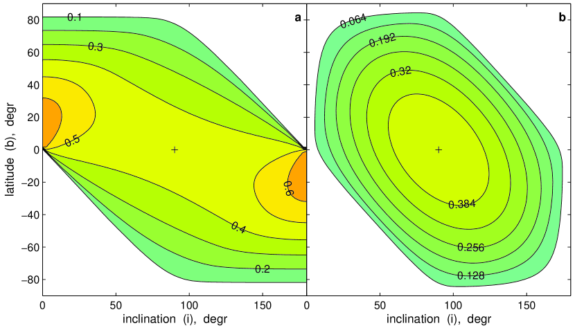
Figure 1: The magnitudes of relative RMS perturbations from a single star spot: a) ratio RMS($\Delta x$)$/$ RMS($\Delta F/F$) in units of apparent stellar radius $R$; b) ratio RMS($\Delta V_{\rm R}$)$/$ RMS($\Delta F/F$) in units of $V_{\rm eq}(1-0.19\sin^{2}b)$. In both cases the values at $i=90\arcdeg$, $b=0\arcdeg$ are 0.448.

3 Comparison with observations

3.1 HD 166435

The star HD 166435 is a solar-type dwarf at 25 pc without conspicuous signs of chromospheric or coronal activity, which nonetheless exhibits large and correlated variations in brightness, radial velocity, and CaII H and K lines (Queloz et al., 2001). Strong evidence is presented in that paper that these periodic variations are caused by a photospheric spot or a group of spots, including analysis of spectral line bisectors. Some confusion with a possible short-period giant planet resulted from the conspicuously large amplitude of the RV variation ($\simeq 200$ m s^-1 peak-to-peak) and the stable phase on a time scale of 30 days. Queloz et al. obtained a projected rotation velocity of $v\,\sin\,i=7.6\pm 0.5$ km s^-1  and a period of 3.7987 d. They estimated a $i=30\arcdeg$ from these data. The shape of the variability curves is consistent with a single dominating spot rotating with this period.

Ignoring the differential rotation term (which is probably small for fast-rotating stars) and setting $\Delta V_{\rm R}$ to 200 m s^-1 from Queloz et al.’s Fig. 8, or 166 m s^-1 from their text, and $\Delta m$ to $0.1$ mag or $0.07$ mag, we derive from Eqs. 3 $\cos\,b=0.286$, $b=73\arcdeg$, or $\cos\,b=0.339$, $b=70\arcdeg$, respectively. This latitude is ambiguous with respect to sign, the possible combinations being $i=30\arcdeg$, $b=70\arcdeg$ (counterclockwise rotation), or $i=150\arcdeg$, $b=-70\arcdeg$ (clockwise rotation). In any case, the center of the spot is close to the pole, and because of the small inclination, circles close to the middle of the visible stellar disk. This is fully consistent with the conclusion by Queloz et al. (2001), which they draw from the smoothness of the variability curves. Finally, using the above estimates for $i$ and $b$, we compute the light curve, which is indeed a smooth sinusoid-like function of time, with a peak-to-peak amplitude of $0.51(1-f_{\rm s})r^{2}$. For a large spot area, the factor $r^{2}$ is interpreted as the fraction of the observed hemisphere covered by the spot. The characteristic contrast ratio of sunspots is 0.2 in the optical passband, which corresponds to an effective temperature of $\sim 4400$ K for the spotted photosphere (Lanza et al., 2008). This yields a striking number for the area of the spot, $r^{2}=0.23$, or an angular radius $\rho=40\arcdeg$. This feature appears to be a dark sea engulfing the pole. Queloz et al. (2001) find that the phase of the RV variation is confined to a $\pm 0.1$ interval (their Fig. 4), which indicates that the feature is stable on a time scale of 2 years, but with considerable internal variations of brightness.

3.2 $\kappa^{1}$ Ceti

The available data for this star relevant to this study include the precision photometric series from MOST and 44 individual RV measurements spread over some 20 years, provided by one of us (DF). The MOST data sets have been carefully analyzed in other papers (Rucinski et al., 2004; Walker et al., 2007; Biazzo et al., 2007), with a firm conclusion that its light curve can be well modeled with a set of two or three dark spots. The periods of rotation range between 8.3 and 9.3 days. The observed peak-to-peak amplitudes in flux are roughly $0.05$ in 2003, but only $\approx 0.02$ in 2004 and 2005. The projected speed of rotation measured by (Valenti & Fischer, 2005), $v\,\sin\,i=5.2\pm 0.5$ km s^-1 implies, from Eq. 3, a RV perturbation $\leq 260$ m s^-1 in 2003 and $\leq 120$ m s^-1 in 2004 and 2005. Due to the sparsity of the RV data, we can not match them directly with the intervals of MOST observations, but we can estimate the amplitude of RV variation over two decades. With the smallest observed value of $-68.56\pm 5.01$ m s^-1, and the largest $+42.50\pm 9.88$ m s^-1, the amplitude is close to the single-spot estimate for the more quiescent periods, but is much smaller than the prediction for 2003. Independent observations by Walker et al. (1995) during 1982–1992 also indicated a peak-to-peak amplitude of $\sim 100$ m s^-1. One possible explanation is that the spots usually reside at high latitudes, which reduces the relative variation in RV because of the $\cos\,b$ factor. The smaller RV variability may also be related to the fact, that two or three spot groups are present on the surface at a time, rather than one single spot. Eqs. 3 can not be simply scaled for the case of multiple spots, because the $\Delta V_{\rm R}$ and $\Delta x$ function of time are symmetric around the central meridian ($C=0$). As a result, two spots well separated in longitude can counterbalance each other, reducing or nearly canceling the net perturbation. Indeed, the detailed modeling by Walker et al. (2007) indicate that large spots frequently occur in the near-polar regions of $\kappa^{1}$ Ceti, and that two or three coexisting spots are spread in longitude, rather than grouped in a confined active area.

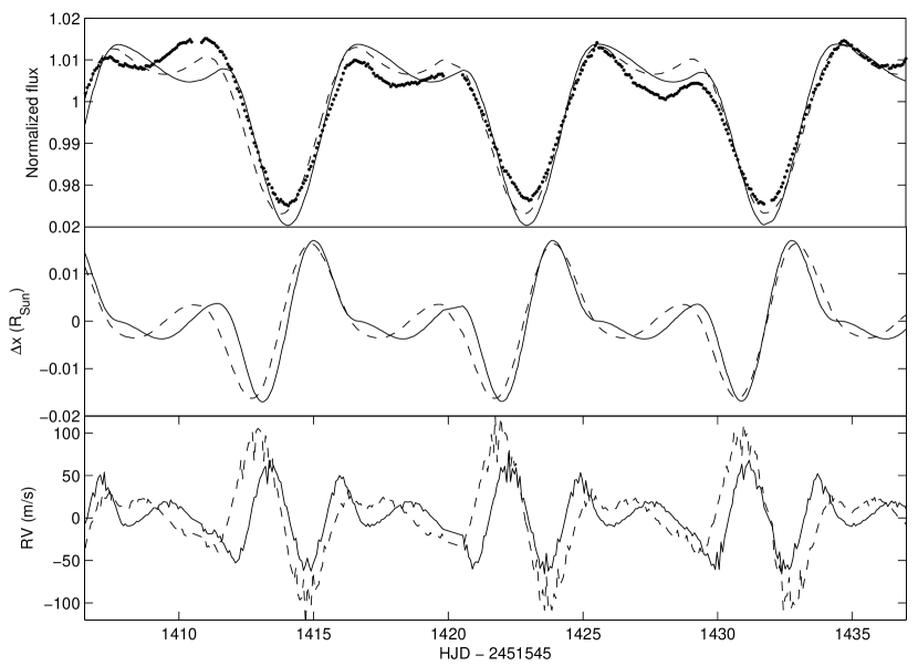
Figure 2: Numerical simulations of variation in relative flux, equatorial shift of the photocenter, and radial velocity of $\kappa^{1}$ Ceti caused by two rotating spots, corresponding to the first segment of observations with MOST in 2003. Our prediction is drawn with a solid line, Walker et al. (2007) results with dashed line, and MOST data with asterisks.

Learning more about the properties of spots on this star requires more accurate computation. One of us (JL) created a code to model differentially rotating star spots and the resulting perturbations of the observable parameters by pixelization of the stellar surface and integration over the visible hemisphere. The free model parameters were optimized on the photometric series of $\kappa^{1}$ Ceti, essentially repeating the study by Walker et al. (2007), but also extending it to astrometric and radial velocity predictions. A detailed description of this model will be published elsewhere, here we only discuss some of the results relevant for this paper. Fig. 2 shows the simulated perturbations from our model, along with the expected perturbations from the model by Walker et al., and the actual light curve from MOST for the segment of 2003. With only two spots in both cases, the goodness of photometric fit is similar with the two models, but our simulation predicts a smaller amplitude of RV variation ($\sim 110$ m s^-1), probably because of a more symmetric configuration of spots. This prediction is in fact consistent with the available RV data. The ratio of simulated variations in $\Delta V_{\rm R}$ and $\Delta x$ is consistent with Eq. 5.

4 The Sun

We estimated in § 2 that the expected RMS jitter in RV for the Sun is $0.38$ m s^-1. The half-amplitude of the reflex motion caused by the Earth orbiting the Sun is slightly less than $0.1$ m s^-1. Does this result imply that detection of Earth-like planets in the habitable zone of Sun-like stars is impossible? This brings up the more subtle issue of the spectral power distribution of starspot jitter. The characteristic period of star spot rotation is 1 month for Solar-type stars, but the orbital periods of habitable planets are of order 1 year. It is therefore not obvious without more detailed analysis that the signal-to-noise ratio will be too small for a confident detection in the frequency domain of interest.

One of us (JC) performed extensive Monte-Carlo simulations for the Sun, which are described in more detail in (Catanzarite et al., 2008). Sunspot groups are generated randomly through a Poisson process, with probability distributions consistent with the current data. The main purpose of this simulation is to faithfully reproduce the power spectrum of the solar irradiance data on a time scale of 30 years. The average number of sunspot groups and the dispersion of lifetimes was adjusted in such a way that the predicted and the observed spectral power of $\Delta F/F$ match closely in the frequency range $10^{-7}$ to $4\times 10^{-8}$ Hz. This gives some assurance that the model predictions can be accurately made for the power spectra of the astrometric and RV jitters. Typical RMS values of jitter predicted by the numerical simulation at $i=90\arcdeg$ are: $0.39$ m s^-1 for RV, $0.97$ $\mu$AU in $x$, and $0.52$ $\mu$AU in $y$, quite close to the analytical estimates in § 2.

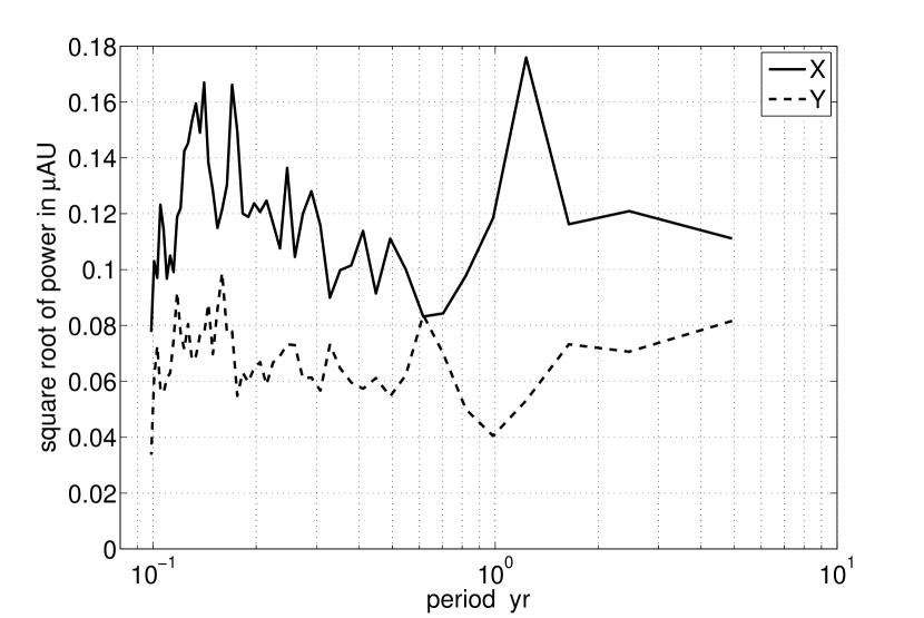
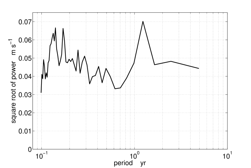
Figure 3: Square root of the spectral power of simulated astrometric (left plot) and radial velocity (right plot) perturbations of the Sun seen at inclination $90\arcdeg$. The X axis is aligned with the equator, and the Y with the rotation axis.

Fig. 3 shows the square root of power in 100 astrometric and radial velocity observations over 5 years simulated for the Sun at $i=90\arcdeg$. The equator is expected to be coplanar with the orbital plane, hence, the exoplanet signal will be present only in the $x$-measurements. The power of spot-related jitter spreads far and wide from the rotation period of 25 days. It peaks between periods of 1 and 2 years, reaching almost $0.18$ $\mu$AU in astrometry. In the worst case, exoplanets with signatures of $0.63$ $\mu$AU or greater can be confidently discovered with SNR$>3.5$ by the astrometric method. The spectrum of the simulated RV variations is practically identical to the spectrum of $x$-jitter, as predicted in § 2. The peak value is $0.07$ m s^-1. The corresponding semiamplitude of exoplanet signature detectable at SNR$=3.5$ is $0.25$ m s^-1.

5 Conclusions

Our results for the Sun are in good agreement with the approximate relations by Eriksson & Lindegren (2007), who estimated a positional standard deviation of 0.7 $\mu$AU. At the same time, their conclusion that ”for most spectral types the astrometric jitter is expected to be of the order of 10 micro-AU or greater” is misleading, because it is largely based on overestimated values of photometric variability from ground-based observations, and it does not differentiate the luminosity classes of giants and dwarfs. It can not be concluded that the Sun is exceptionally inactive compared to its peers just because the ultra-precise solar irradiance data, such as PMOD or SOHO, reveal a much smaller scatter than the inferior photometric data for other stars. We investigated the indices of chromospheric activity ($\log R^{\prime}_{\rm HK}$) and available rotation periods for some 80 SIM targets, and found that half of them should rotate with the same rate as the Sun, or slower.

Hall et al. (2000) presented a detailed study of variability of solar-type stars and its relation to the index of chromospheric activity $\log R^{\prime}_{\rm HK}$, based on 14 years of photometric and spectroscopic observations. They found that the Sun at $\log R^{\prime}_{\rm HK}=-4.96$ is not more variable than its F-G peers at the low end of the activity distribution. Given that most Solar-type stars exhibit similar low levels of chromospheric activity (Gray et al., 2003), we expect that finding stars with levels of jitter similar to, or lower than the Sun, should not be a problem. Low-jitter, stable stars are common and plentiful, which augurs well for the prospects of finding small, rocky planets with Kepler (Batalha et al., 2002).

Table 1: Observable signals and star spot jitters for an Earth-like planet orbiting a typical dwarf star at 10 pc.

Star type	Sun	F5V	K5V
Rotation period, d	25.4	18	30
Astrometric signal, $\mu$as	0.30	0.23	0.45
RV signal, m s-1	0.089	0.078	0.109
Astrometric jitter, $\mu$as	0.087	0.113	0.063
RV jitter, m s-1	0.38	0.69	0.23
Astrometric SNR	3.4	2.0	7.1
RV SNR	0.23	0.11	0.47

The SIM Lite Astrometric Observatory (formerly known as the Space Interferometry Mission) will achieve a single-measurement accuracy of 1 $\mu$as or better in the differential regime of observation (Unwin et al., 2008; Davidson et al., 2009). Several previous studies have addressed SIM’s exoplanet detection and orbital characterization capabilities (Catanzarite et al., 2006, and references therein). The ”Tier 1” program includes $\sim 60$ nearby stars for which the astrometric signature of a terrestrial habitable planet is large enough to be confidently measured by SIM. The recently completed double-blind test (Traub et al., 2009) demonstrated that Earth-like planets around nearby stars can be discovered and measured even in complex planetary systems. In this paper, we are concerned with the more general question of the ultimate limit to planet detectability set by the activity-related jitter. Assuming that the instrumentation progresses to levels where observational noise becomes insignificant, which technique holds the best prospects for detection of habitable Earth-like planets? Table 1 summarizes the expected RMS jitter and the exoplanet signal for three typical nearby stars. In all cases, the solar spot filling factor ($r^{2}$) is assumed. The signal-to-noise ratios (SNR) per observation include only the star spot jitter. Note that the astrometric SNR in this case is independent of the distance to the host star, because both the signal and the star spot jitter are inversely proportional to distance. As a measure of the relative sensitivity of the two methods, the ratio of the SNR values for a given star is independent of the planet mass or the filling factor to first-order approximation. The physical radius of the star and the period of rotation are the two parameters with the largest impact on the relative sensitivity, but their combined effect is rather modest for normal stars, as is seen in the Table. Therefore, in the ultimate limit of exoplanet detection defined by intrinsic astrophysical perturbations, the astrometric method is at least an order of magnitude more sensitive than the Doppler technique for most nearby solar-type stars.

References

- Batalha et al. (2002) Batalha, N.M., et al. 2002, ESA-SP 485, 35
- Benedict et al. (2006) Benedict, G.F., et al. 2006, AJ, 132, 2206
- Biazzo et al. (2007) Biazzo, K., et al. 2007, ApJ, 656, 474
- Catanzarite et al. (2008) Catanzarite, C., Law, N., & Shao, M., 2008, Proc SPIE, 7013, 70132K
- Catanzarite et al. (2006) Catanzarite, C., et al. 2006, PASP, 118, 1319
- Davidson et al. (2009) Davidson, J., et al. 2009, SIM Lite Astrometric Observatory, NASA, JPL 400-1360 (available upon request from authors)
- Eriksson & Lindegren (2007) Eriksson, U., & Lindegren, L. 2007, A&A, 476, 1389
- Fröhlich & Lean (1998) Fröhlich, C., & Lean, J. 1998, Geophysical Research Letters, 25(23), 4377
- Gray et al. (2003) Gray, R.O., et al. 2003, AJ, 126, 2048
- Hall et al. (2000) Hall, J.C., et al. 2009, AJ, 138, 312
- Kitchatinov (2005) Kitchatinov, L.L., 2005, Phys. Uspekhi, 48(5), 449
- Lanza et al. (2008) Lanza, A.F., De Martino, C. & Rodonò, M. 2008, New Astronomy, 13, 77
- Mayor & Udry (2008) Mayor, M., & Udry, S. 2008, Phys. Scr., T130, 014010
- Newton & Nunn (1951) Newton, H.W., & Nunn, M.L. 1951, MNRAS, 111, 413
- Pravdo & Shaklan (2009) Pravdo, S.H., & Shaklan, S.A. 2009, ApJ, 700, 623
- Queloz et al. (2001) Queloz, D., et al. 2001, A&A, 379, 279
- Rucinski et al. (2004) Rucinski, S.M., et al., 2004, PASP, 116, 1093
- Traub et al. (2009) Traub, W.A., et al., 2009, BAAS, 41, 267
- Unwin et al. (2008) Unwin, S.C., et al. 2008, PASP, 120, 38
- Valenti & Fischer (2005) Valenti, J.A., & Fischer, D.A. 2005, ApJS, 159, 141
- Walker et al. (1995) Walker, G.A.H., et al. 1995, Icarus, 116, 359
- Walker et al. (2007) Walker, G.A.H., et al. 2007, ApJ, 659, 1611