An axisymmetric generalized harmonic evolution code

Abstract

We describe the first axisymmetric numerical code based on the generalized harmonic formulation of the Einstein equations, which is regular at the axis. We test the code by investigating gravitational collapse of distributions of complex scalar field in a Kaluza-Klein spacetime. One of the key issues of the harmonic formulation is the choice of the gauge source functions, and we conclude that a damped wave gauge is remarkably robust in this case. Our preliminary study indicates that evolution of regular initial data leads to formation both of black holes with spherical and cylindrical horizon topologies. Intriguingly, we find evidence that near threshold for black hole formation the number of outcomes proliferates. Specifically, the collapsing matter splits into individual pulses, two of which travel in the opposite directions along the compact dimension and one which is ejected radially from the axis. Depending on the initial conditions, a curvature singularity develops inside the pulses.

I Introduction

In general, a detailed investigation of fully nonlinear gravitational dynamics is impossible by other than numerical means. Luckily, the numerical methods have recently reached the level of maturity that finally allows addressing many long-standing puzzles. Perhaps the most remarkable is the progress achieved in solving a general-relativistic two-body problem—the coalescence of black holes FP2 ; FP1 ; FP3 ; RIT ; nasa ; AEI ; CaltechCornell . Driven by the gravitational wave detection prospects, the problem of the collision of two black holes or neutron stars continues to be the central front where an overwhelming majority of numerical relativity research is done. Fortunately, the computational methods employed there are portable and—as demonstrated below—can readily be applied on other problems of interest.

The success of the numerical simulations was backed up by a parallel development of the software and the hardware, which provided the necessary computational resources. The rapid hardware evolution combined with the persisting regularity problems in axial symmetry eventually led to a direct transition from highly symmetrical spherical configurations to fully general 3D situations without any symmetries at all, essentially bypassing the intermediate axisymmetric case. However, here we argue that important theoretical and practical reasons exist to explore axisymmetry better, and we describe a new regular numerical code that, we believe, will be capable of achieving this. 

Before describing any concrete setup we would point out one important possible use of an axisymmetric code, specifically, that it can be regarded as an efficient “calibration tool” for more general 3D codes. Indeed, we expect that an intrinsically axisymmetric code applied to, say, the head-on collision of two black holes would be capable of following the evolution and the resulting gravitational radiation more accurately compared to Cartesian 3D numerical implementations, both because of explicit use of the symmetry and since higher numerical resolution can be employed for given hardware resources.

Several interesting open problems arise in axisymmetric gravitational collapse situations. In particular, it remains unclear whether or not the weak cosmic censorship is violated in collapse of prolate Brill waves BrillWaves ; Rinne_axi_1 . An independent observation of universality in critical collapse of gravitational waves AbrahamsEvans is pending, as well as further investigation of the non-spherical unstable mode that apparently shows up at threshold for black hole formation in axisymmetric collapse of a scalar field crit_collapse_axi . A basic problem of mathematical relativity concerning the stability of black holes with respect to nonlinear axisymmetric perturbations, can be equivalently addressed in a collapse situation by computing how fast a newly formed black hole radiates away higher multipole moments.

In addition, we shall mention other, rarely cited in the context of numerical relativity, axisymmetric systems which are of great interest in theoretical work on higher-dimensional gravity. One of the most basic motivations for studying higher-dimensional spacetimes relies on the observation that the Einstein equations, describing classical General Relativity (GR), are independent of the spacetime dimension. Nevertheless, certain properties of the solutions to these equations vary dramatically with the dimension. A striking example is that axisymmetric black holes in dimensions greater than four do not necessarily have spherical horizons, but also admit horizons of toroidal topology BlackRing . Moreover, and in sharp contrast to their four-dimensional counterparts, higher dimensional black holes do not respect the Kerr limit MP , and they are unstable in certain range of parameters GL . One of the fundamental unresolved puzzles HM ; Choptuik_BS is whether or not the instability leads to fragmentation of the horizon and exposition of the inner singularity, hence violating the cosmic censorship hypothesis.

Since it is unlikely that any of these these problems can be addressed analytically in a systematic manner, we turn to computational methods. However, solving the Einstein equations numerically is notoriously difficult and depends crucially on the way these equations are formulated and evolved. In this paper we focus on the generalized harmonic (GH) formulation Friedrich85 ; Friedrich96 ; Garfinkle2001 that has recently gained popularity because of its great success in the simulations of black hole binaries FP2 ; FP3 ; CaltechCornell ; FP1 ; Lindblom_etal .

In a nutshell, the GH approach is a way to write the field equations such that the resulting system is manifestly hyperbolic, taking the form of a set of quasilinear wave equations for the metric components. As the name suggests, the GH method generalizes the harmonic approach, which achieves strong hyperbolicity by choosing the harmonic spacetime coordinates. In the GH approach much of the coordinate freedom is regained through the introduction of certain gauge source functions, which also maintains the desirable property of strong hyperbolicity of the field equations. In fact, the source functions can be thought of as representing the coordinate freedom of the Einstein equations, and when constructing solutions of the equations, via an initial value approach, for example, they must be completely specified in some fashion. Choosing the source functions in a controlled way is a key issue of the GH technique and after testing several recent prescription, we conclude that a damped wave gauge LS is remarkably robust in collapse situations.

Applications of the GH approach in spherically-symmetric situations were studied in SorkinChoptuik and here we employ the method in axisymmetry. In both cases it is natural to use coordinates in which the symmetries of the spacetime are explicit. However, these coordinates, are formally singular: at the origin in spherical symmetry and on the axis in axial symmetry. Thus, the field equations have to be regularized in numerical implementations; here we describe a regularization procedure that is compatible with the GH formulation.

Our numerical implementation of the GH system is a free evolution code that advances initial data by solving a set of wave equations. In addition, there are also constraint equations that must be satisfied during the evolution. Although the constraints are consistently preserved in the GH approach in the continuum limit, in numerical computations at finite resolution, constraint violations generically develop. In order to maintain stability these deviations must be damped and we discuss an effective method that achieves this.

Having in mind implications for higher-dimensional GR we test our new code by studying gravitational collapse of a complex scalar field in a $D$-dimensional Kaluza-Klein (KK) spacetime. This background, which has a single compact extra dimension curled into a circle, is a classical example of a higher-dimensional compactified spacetime that in certain limits can appear four dimensional, for example when the size of the compact dimension is small. Assuming spherical symmetry in the infinite $(D-2)$-dimensional portion of the space makes the problem 2+1 that depends on time and two spatial coordinates: one in the radial direction, and one along the KK circle.

We perform a series of numerical simulations where the initial distribution of the scalar matter is freely specified and the outcome of the evolution depends on the “strength” of the initial data as well as on its topology. The weak data correspond to the dispersion of relatively dilute pulses, while a typical strong data configuration leads to black hole formation or nearly does so. Our preliminary results indicate a wide range of the black hole forming scenarios, including how many holes form and of what topology. For instance, a static distribution of matter centered at the axis and localized in the KK direction with the energy-density above certain threshold collapses to form a black hole with a quasi-cylindrical horizon, smeared along the extra-dimension. Data with the energy-density below this threshold evolve to form a quasi-spherical horizon centered around the initial matter distribution. By further reducing the density we find that resulting black holes become progressively smaller, and at some critical density a pulse of matter is emitted radially away from the axis and a curvature singularity develops inside it. We find that for slightly lower initial densities the evolving matter splits into several pulses and two of them individually collapse to form the singularities moving apart along the KK dimension. Finally, when the initial matter distribution becomes dilute below a certain limit, no black holes or curvature singularities are created.

In the next section we describe the class of effectively 2+1 dimensional models where our code can currently be applied. In Sec. III we present the basic formulas of the GH formulation and discuss the constraints and a method to damp their violations. We describe an axis regularization in Sec. III.1 and boundary conditions in Sec. III.2. Although, in this work we integrate full $D$-dimensional equations, in the Appendix we describe an alternative approach—one that uses a dimensional reduction on the symmetry and integrates the reduced 2+1 equations—and compare its performance with ours. Coordinate conditions and the initial data problem are formulated in Secs. III.3 and III.4, respectively. We use several diagnostics to probe the spacetimes that we construct, including computation of asymptotic measurables and apparent horizons, and describe that in Sec. III.5. After elaborating on our numerical algorithm in Sec. IV we test its performance in Sec. V, giving detailed accounts of various aspects, such as specific coordinate choices, constraint damping, numerical dissipation, and convergence. We conclude in Sec. V.4, outline possibilities of improvement, and discuss some future prospects.

II The Setup

We consider a $D$-dimensional spacetime that possesses the $O(D-2)$ isometry group. We will further assume that the corresponding Killing vectors are orthogonal to the closed hypersurface they generate. The symmetry reduces the problem to effectively 2+1, which depends on time, $t$, and two spatial dimensions that we denote by $r$ and $z$. The spatial coordinates can be either infinite or finite. For instance, taking $D=4$ and assuming asymptotic flatness correspond to the usual four-dimensional axially-symmetric situation without angular momentum, while setting $D=5$ and assuming periodic $z$ and infinite $r$ can describe dynamics in a five-dimensional Kaluza-Klein background.

The most general $D$-dimensional line element with these isometries can be written as

$$ds^{2} = g_{\mu\nu}\,dx^{\mu}dx^{\nu}=$$ (1)

$$= g_{ab}\,dx^{a}dx^{b}+e^{2\,S}\,r^{2}\,d\Omega_{n}^{2}.$$

Here $g_{\mu\nu}$ is the $D$-dimensional metric, $d\Omega_{n}^{2}$ is the metric on a unit n-sphere, $n\equiv D-3$, $a,b=0,1,2$ running over $\{t,r,z\}$, and the $3$-metric $g_{ab}$ and scalar $S$ are functions of $t,r$ and $z$, alone.

We take a complex, minimally coupled to gravity scalar field to represent the matter of the theory and write the total action of the system as

$$S = S_{EH}+S_{\Phi}=$$ (2)

$$= \frac{1}{16\pi G_{N}}\int\sqrt{-g_{D}}\Big{[}R_{D}-$$

$$- g^{\mu\nu}\,{\partial}_{(\mu}\Phi\,{\partial}_{\nu)}\Phi^{*}+2\,V(|\Phi|)\Big{]}dx^{D},$$

where $G_{N}$ is the $D$-dimensional Newton constant.

In the next section we will describe our strategy to solving the equations derived from this action. We will focus on asymptotically flat spacetimes times a circle (having the topology $\mathbb{R}^{D-2,1}\times S^{1}$) but remark that asymptotically de Sitter (dS) and anti-de Sitter (AdS) spacetime are also included in our model (2) when the potential of the scalar field satisfies $V(0)\rightarrow\Lambda$ with positive and negative $\Lambda$, respectively.

III Generalized-harmonic formulation and its reduction to 2D case

In order to numerically solve the Einstein equations derived from (2), we use the generalized harmonic formulation. To make the description as self-contained as possible, we summarize below basic facts regarding the approach, (more details can be found in e.g. FP1 ; Lindblom_etal ; SorkinChoptuik ) and adapt it to the 2+1 situation of interest.

We begin by noting that whenever isometries are present one could perform a Kaluza-Klein reduction on them, and in our case (2) the reduction yields lower-dimensional, 2+1 Einstein equations coupled to the scalar, which is related to the size of the $n$-sphere, and the matter. Initially, we had indeed performed such a reduction and coded the reduced equations; see the Appendix A for details and comparison of the methods. However, after experimenting with the reduced and the full $D$-dimensional versions of the equations, we found that numerical solution of the latter is generically more stable. Therefore, in what follows we adopt the unreduced approach.

The Einstein equations on a $D$-dimensional spacetime obtained by varying the action (2) can be written in the form

$$R_{\mu\nu}=8\pi G_{N}\bar{T}_{\mu\nu}\equiv 8\pi G_{N}\left(T_{\mu\nu}-\frac{1}{D-2}g_{\mu\nu}T\right),$$ (3)

where $R_{\mu\nu}$ is the Ricci tensor, $T_{\mu\nu}={\partial}_{(\mu}\Phi\,{\partial}_{\nu)}\Phi^{*}-(1/2)g_{\mu\nu}(|{\partial}\Phi|^{2}+2\,V)$ is the energy-momentum tensor of the matter with trace $T$. Hereafter we use units in which the $D$-dimensional Newton constant satisfies $8\pi\,G_{N}=1$.

The Ricci tensor that appears in the left-hand-side of (3) contains various second derivatives of the metric components $g_{\mu\nu}$: these second derivatives collectively constitute the principal part of $R_{\mu\nu}$, viewed as an operator on $g_{\mu\nu}$. This principal part can be decomposed into a term $g^{\alpha\beta}{\partial}_{\alpha\beta}g_{\mu\nu}$, plus mixed derivatives of the form $g^{\alpha\gamma}{\partial}_{\alpha\mu}g_{\gamma\nu}$. Without the mixed derivatives, (3) would represent manifestly (and strongly) hyperbolic wave equations for the $g_{\mu\nu}$ Friedrich96 . One can view the GH formulation of general relativity as a particular method that eliminates the mixed second derivatives appearing in (3); see  Friedrich85 ; Garfinkle2001 ; FP1 ; FP3 ; Lindblom_etal .

One requires that the coordinates satisfy

$$\Box x^{\alpha}=-\Gamma^{\alpha}=H^{\alpha},$$ (4)

where $H_{\alpha}\equiv g_{\alpha\beta}H^{\beta}$ are arbitrary “gauge source functions” which are to be viewed as specified quantities, and $-\Gamma^{\alpha}\equiv\Gamma^{\alpha}_{\mu\nu}g^{\mu\nu}$ are the contracted Christoffel symbols. One defines the GH constraint

$$C^{\alpha}\equiv H^{\alpha}-\Box x^{\alpha},$$ (5)

which clearly must vanish provided (4) holds, and then modifies the Einstein equations as follows:

$$R_{\mu\nu}-C_{(\mu;\nu)}=\bar{T}_{\mu\nu}.$$ (6)

This last equation can be written more explicitly as

$$- {1\over 2}g^{\alpha\beta}g_{\mu\nu,\alpha\beta}-{g^{\alpha\beta}}_{(,\mu}g_{\nu)\beta,\alpha}-H_{(\mu,\nu)}+H_{\beta}\Gamma^{\beta}_{\mu\nu}-$$ (7)

$$- \Gamma^{\alpha}_{\nu\beta}\Gamma^{\beta}_{\mu\alpha}={\partial}_{(a}\Phi\,{\partial}_{b)}\Phi^{*}+\frac{2}{D-2}g_{ab}\,V.$$

Now, provided that $H_{\alpha}$ are functions of the coordinates and the metric only, but not of the metric derivatives—namely $H_{\alpha}=H_{\alpha}(x^{\mu},g)$—the field equations (7) form a manifestly hyperbolic system. The source functions $H_{\alpha}$ are arbitrary at this stage and their specification is equivalent to choosing the coordinate system (“fixing the gauge”). Determining an effective prescription for the source functions is thus crucial for the efficacy of the GH approach, and our strategies for fixing the $H_{\alpha}$ are discussed in Sec. III.3.

After the coordinates have been chosen, we integrate the equations forward in time. Consistency of the scheme requires that the GH constraint (5) be preserved in time. The contracted Bianchi identities guarantee that this is indeed the case, since, using those identities, one can show FP1 ; Lindblom_etal that $C^{\alpha}$ itself satisfies a wave equation,

$$\Box C^{\alpha}+{R^{\alpha}}_{\nu}\,C^{\nu}=0.$$ (8)

Thus, assuming that the evolution is generated from an initial hypersurface on which $C^{\alpha}={\partial}_{t}C^{\alpha}=0$, and constraint preserving boundary conditions are used during the evolution, (8) guarantees that $C^{\alpha}=0$ for all future (or past) times.

Although the GH constraint is preserved at the continuum level, in numerical calculations, where equations are discretized on a lattice the constraint cannot be expected to hold exactly. It appears that numerical solutions of (7) can admit “constraint violating modes”, with the result that the desired continuum solution is not obtained in the limit of vanishing mesh size. However, an effective way of preventing the development of such modes in numerical calculations exists: one adds terms to the field equations that are explicitly designed to damp constraint violations (see e.g. KST ). Following the approach of Pretorius FP1 ; FP3 that builds on earlier works gm_sys ; Gundlachetal we define the constraint damping terms

$$Z_{\mu\nu}\equiv\kappa\left(n_{(\mu}{\cal C}_{\nu)}-{1\over 2}g_{\mu\nu}\,n^{\beta}\,{\cal C}_{\beta}\right),$$ (9)

and solve the modified equations of the form

$$R_{\mu\nu}-C_{(\mu;\nu)}+Z_{\mu\nu}=\bar{T}_{\mu\nu}.$$ (10)

Here, $n_{\mu}$ is the unit time-like vector normal to the $t={\rm const.}$ hypersurfaces, that can be written as

$$n_{\mu}\equiv-\left(1/\sqrt{-g^{00}}\right){\partial}_{\mu}t,$$ (11)

and $\kappa$ is an adjustable parameter that controls the damping timescale. Specifically, it is shown in Gundlachetal that small constraint perturbations about Minkowski background decay exponentially with a characteristic timescale of order $\kappa$. We note that the constraint damping term contains only first derivatives of the metric and hence does not affect the principal (hyperbolic) part of the equations.

III.1 Regularization of the axis, $r=0$

Having described the GH formulation, we now specialize to the symmetric case. We note first that in our coordinates (1) adapted to the symmetry the line element of the flat spacetime becomes

$$ds^{2}=-dt^{2}+dr^{2}+dz^{2}+r^{2}\,d\Omega_{n}^{2},$$ (12)

and that in this case the source function (4) does not vanish but becomes

$$H^{\rm Mink}_{\mu}=-\Gamma^{\rm Mink}_{\mu}=$$

$$=(0,\frac{n}{r},0,(n-1)\,\cot\theta_{1},\dots,\cot\theta_{n-1},0),$$ (13)

where $\theta_{i}$ are angular coordinates of the sphere’s line element $d\Omega_{n}^{2}$. Since near the axis a general spacetime is locally flat, the radial component of the source function is generically singular at $r=0$, diverging as $n/r$. To regularize this radial component, we thus subtract the singular background contribution by transforming

$$H_{\alpha}\to H_{\alpha}+\delta^{1}_{\alpha}\,H_{1}^{\rm Mink}$$ (14)

and prescribe gauge conditions using the regular sources.

Invariance of the line element (1) under the reflection $r\rightarrow-r$ in our case implies that the metric components $g_{01}$ and $g_{12}$ are odd functions of $r$, while $g_{00},g_{11},g_{22},g_{02},S$ and $\Phi$ are even in $r$. The GH constraint (4) then dictates that $H_{1}$, regularized via (14) is an odd function of $r$, while $H_{0}$ and $H_{2}$ are even in $r$.

Moreover, the requirement that the surface area of an $n$-sphere must vanish at the axis implies $g_{11}(t,0,z)=\exp[2\,S(t,0,z)]$. We note that this is an extra condition on $S$, which thus has to satisfy both this relation, as well as the constraint that it have vanishing radial derivative at $r=0$—specifically that $g_{11}-\exp(2\,S)=O(r^{2})$. Therefore, at $r=0$ we essentially have three conditions on the two fields $S$ and $g_{11}$. In the continuum, and given regular initial data, the evolution equations will preserve regularity, however, in a finite-differencing numerical code this will be true only up to discretization errors. As a general rule-of-thumb, the number of boundary conditions should be equal to the number of evolved variables in order to avoid regularity problems and divergences of a numerical implementation.

An elegant way to deal with this regularity issue involves definition of a new variable, $\lambda$, :

$$\lambda\equiv\frac{g_{11}-e^{2\,S}}{r}.$$ (15)

At the axis one then has $\lambda\sim O(r)$. Therefore, after changing variables from $S$ to $\lambda$ by using $S=(1/2)\log(g_{11}-r\,\lambda)$ in all equations, and imposing $\lambda(t,0,z)=0$ at the axis, one ends up with a system where there is no over-constraining due to the demand of regularity at $r=0$. Crucially, we note that the hyperbolicity of the GH system is not affected by the change of variables.

While we note that a more straightforward regularization method that maintains $S$ as a fundamental dynamical variable and employs analytical Taylor-series expansion of the equations in the vicinity of $r=0$ can also be used in simulations, its reliability degrades in the strong field regime, where the regularization that uses $\lambda$ remains consistently accurate.

III.2 The field equations and Kaluza-Klein boundary conditions

With the metric ansatz (1) and the regularized source function (14), our equations become 8 equations for 8 variables: six components of the 3-metric $g_{ab}$, and real and complex scalars $\lambda$ and $\Phi$ correspondingly. Schematically the system can be written as

$$-{1\over 2}g^{cd}g_{ab,cd} - H_{(a,b)}+\dots=$$ (16)

$$= {\partial}_{(a}\Phi\,{\partial}_{b)}\Phi^{*}+\frac{2}{D-2}g_{ab}V,$$

$$-{1\over 2}g^{cd}\lambda_{,cd} - {1\over 2}\,\frac{{\partial}_{r}\,H_{1}}{r}+\dots=$$ (17)

$$= \frac{2}{D-2}\,V\,\lambda+\frac{|{\partial}_{r}\Phi|^{2}}{r},$$

$$g^{cd}\Phi_{,cd} + \dots={\partial}V/{\partial}\Phi^{*}.$$ (18)

Here ellipses denote terms that may contain the metric and it derivatives and/or the source functions, in various combinations. These equations are to be evolved forward in time starting from the initial ($t=0$) time slice, where values for the fields and their first time derivatives must be prescribed.

In order to completely specify the problem we have to provide boundary conditions which the above equations are subject to. In this paper we will be interested in a $D$-dimensional Kaluza-Klein spacetime of topology ${\mathbb{R}}^{D-2,1}\times S_{z}^{1}$, where the $z$ direction is considered periodic with asymptotic length ${\hat{L}}$ namely that $z\sim z+{\hat{L}}$, and for the future use we also define half-period $L\equiv{\hat{L}}/2$. Asymptotically, this spacetime becomes Minkowski times the compact circle and the corresponding boundary conditions are

$$g_{ab}\rightarrow\eta_{ab},~{}~{}~{}\lambda\rightarrow 0,~{}~{}~{}\Phi\rightarrow 0~{}~{}~{}H_{a}\rightarrow 0.$$ (19)

III.3 Coordinate conditions

As we have already mentioned, fixing the coordinates in the GH approach amounts to specifying the source functions $H_{a}$. The choice that we find to perform best in our case is a variant of the damped-wave gauge (DWG) condition proposed recently in LS (see also PretoriusChoptuik_coll )

$$F_{a}=2\,\mu_{1}\,\log\left(\frac{\gamma^{p}}{\alpha}\right)\,n_{a}-2\,\mu_{2}\,\alpha^{-1}\,\gamma_{ai}\,\beta^{i},$$ (20)

where $\gamma_{ab}=g_{ab}+n_{a}n_{b}$ is the spatial metric whose determinant $\gamma\equiv det\,\gamma_{ij}=(g_{11}\,g_{22}-g_{12}^{2})\,\exp(n\,S)$ has the factor $r^{n}$ removed in accordance with the regularization (14), and $\mu_{1,2}$ and $p$ are free parameters. Since the gauge function (20) depends only on the metric, we can simply set $H_{a}=F_{a}$ without destroying hyperbolicity of our system. Below we refer to this approach as the algebraic DWG condition.

An alternative method that preserves the hyperbolicity was originally devised by Pretorius for binary black hole simulations FP2 ; FP3 and has also proven useful in the studies of the gravitational collapse of scalar field in spherical symmetry SorkinChoptuik . This strategy elevates the status of the $H_{a}$ to independent dynamical variables that satisfy time-dependent partial differential equations. The evolution equations for the $H_{a}$ are designed so that the ADM kinematic variables—lapse $\alpha$ and shift $\beta^{i}$ which (implicitly) result from the time development—have certain desirable properties. For example, the equation for $H_{0}$ is tailored in an attempt to keep the value of the lapse function of order unity everywhere—including near the surfaces of the black holes—during the evolution.

One specific prescription for achieving this type of control evolves the gauge source functions according to

$$\Box H_{t} = -\xi_{1}\,\frac{\alpha-\alpha_{0}}{\alpha^{q}}+\xi_{2}\,H_{t,\mu}n^{\mu},$$

$$H_{i} = 0,$$ (21)

where $\Box$ is the covariant wave operator, and $\alpha_{0},\xi_{1},\xi_{2}$ and $q$ are adjustable constants. Thus the temporal source function satisfies a wave equation similar to those that govern the metric components in the system (10). The first term on the right-hand-side of (III.3) is designed to “drive” $H_{t}$ to a value that results in a lapse that is approximately $\alpha_{0}$. The second, “frictional” term tends to confine $H_{t}$ to this value. For the case of the spatial coordinates, Pretorius found that the simplest choice of spatially harmonic gauge, $H_{i}=0,$ was sufficient in simulations of binary black hole collisions. A slight generalization of this technique was considered in Scheel_etal where instead of using $H_{i}=0$, the spatial components of the source functions are evolved according to

$$\Box H_{i}=-\xi_{3}\,\frac{\beta_{i}}{\alpha^{2}}+\xi_{2}\,H_{i,\mu}n^{\mu}$$ (22)

where $\xi_{3}$ is an additional parameter.

Variants of gauge drivers were further investigated in the recent Lindblom_etal_gauge ; SorkinChoptuik ; LS . Specifically in LS the following hyperbolic first-order drivers were proposed

$${\partial}_{t}H_{a}-\beta^{i}{\partial}_{i}H_{a}=-\nu\,(H_{a}-F_{a})+W_{a},$$

$${\partial}_{t}W_{a}+\eta\,W_{a}=-\eta\,\beta^{i}{\partial}_{i}H_{a},$$ (23)

such that all time-independent solutions of this system satisfy $H_{a}=F_{a}$, where $F_{a}$ are certain predetermined target gauge functions, for instance (20), and the parameters $\nu$ and $\eta$ are freely specified.

In Sec. V.1 we compare the performance of these strategies and argue that in collapse situations the algebraic DWG approach is the most robust of all. Namely, it does not require an extensive fine-tuning of parameters, and it is long-term stable.

III.4 Initial data

We now consider specification of initial data, which are values for the fields and their first time derivatives at $t=0$. For simplicity we restrict attention to time-symmetric initial conditions for the metric and $|\Phi|$.

Given this assumption, initial data for the scalar field reduces to the specification of $\Phi(0,r,z)$, which we take to have the form of a generalized Gaussian,

$$\Phi(0,r,z)=\Phi_{0}\,e^{-\left[(1-e_{r}^{2})(r-r_{0})^{2}+(1-e_{z}^{2})(z-z_{0})^{2}\right]/\Delta^{2}}$$ (24)

where $\Phi_{0}=|\Phi_{0}|\exp(i\,\varphi)$ is a complex amplitude and $r_{0},z_{0},e_{r},e_{z},\Delta$ and $\varphi$ are real adjustable parameters, supplemented by the choice

$${\partial}_{t}\Phi(0,r,z)=i\,\omega\,\Phi(0,r,z),$$ (25)

that satisfies ${\partial}_{t}|\Phi|_{t=0}=0$, where $\omega$ is another parameter.

The momentum constraint is satisfied for our initial data, and writing the initial metric as

$$ds^{2}=-\alpha^{2}dt^{2}+\psi^{4}\left(dr^{2}+dz^{2}+r^{2}d\Omega^{2}_{n}\right),$$ (26)

one can show that the Hamiltonian constraint becomes an elliptic equation for $\psi(0,r,z)$

$${\partial}_{r}^{2}\psi+{\partial}_{z}^{2}\psi+\frac{n}{r}{\partial}_{r}\psi+\frac{n-1}{\psi}\left[({\partial}_{r}\psi)^{2}+({\partial}_{z}\psi)^{2}\right]+$$

$$+\frac{\psi}{2\,(n+1)}\Big{[}{1\over 2}\left(|{\partial}_{r}\Phi|^{2}+|{\partial}_{z}\Phi|^{2}+\alpha^{-2}\psi^{4}\omega^{2}|\Phi|^{2}\right)+$$

$$+\psi^{4}V\Big{]}=0,$$ (27)

that is subject to the boundary conditions, ${\partial}_{r}\psi|_{r=0}=0,~{}{\partial}_{z}\psi|_{z=0}={\partial}_{z}\psi|_{z=L}=0$ and $\psi|_{r\to\infty}=1$.

We will assume initial harmonic coordinates, which implies, see (4), that the lapse can be determined in terms of $\psi$ as

$$\alpha(0,r,z)=\psi^{2\,n}.$$ (28)

After substituting this into equation (III.4) we solve for $\psi$ and initialize our basic variables and their derivatives:

$$g_{ij}(0,r,z) = \psi^{4}\delta_{ij},~{}~{}\lambda(0,r,z)=0,$$

$${\partial}_{t}g_{ij}(0,r,z) = {\partial}_{t}\lambda(0,r,z)=0.$$ (29)

We finally note that in order to use the DWG conditions correctly, we have to smooth out the transition from initially harmonic to later DWG coordinates. As described in Sec. V.1 this can be done stably by multiplying $F_{a}$ in (20) by a time-dependent factor that gradually grows from 0 to 1. For the driver version of DWG we also initialize ${\partial}_{t}W=W=0$ at $t=0$.

III.5 Spacetime diagnostics

We employ several diagnostics in order to probe the geometry of the spacetimes we construct.

III.5.1 Asymptotic charges: Mass and tension.

Far away from an isolated system a natural radial coordinate is well defined by comparison with the flat background, and the charges that characterize the solution can be found from the asymptotic radial behavior of the metric functions. In asymptotically flat spacetimes with no angular momentum there is exactly one charge: the ADM mass. However, in our system with the extra compact dimension, the tension, associated with varying the length of the compact direction, can also be defined. A derivation of this result can be found in KolSorkinPiran1 ; HO1 , but here we note why the appearance of an additional charge could be expected. Asymptotically the metric becomes $z$-independent since from the lower-dimensional perspective the $z$-dependent Kaluza-Klein modes are massive (with the discrete masses $m_{n}=2\pi\,n/L,~{}n>0$) and decay exponentially $\sim\exp(-m_{n}\,r)$. In this situation asymptotic Kaluza-Klein reduction is possible with the result that $g_{zz}$ behaves effectively as a scalar field that carries an (unconserved) charge. Designating the asymptotic fall-off of the metric functions $g_{tt}$ and $g_{zz}$ as

$$g_{tt} = -1+\frac{2\,a}{r^{D-4}},$$

$$g_{zz} = 1+\frac{2\,b}{r^{D-4}},$$ (30)

the mass and tension of the solutions are defined as KolSorkinPiran1 ; HO1

$$\left[\begin{array}[]{c}m\\ \tau\,{\hat{L}}\\ \end{array}\right]={\Omega_{n}\over 8\pi(G_{D}/{\hat{L}})}\left[\begin{array}[]{cc}n&-1\\ 1&-n\\ \end{array}\right]\,\left[\begin{array}[]{c}a\\ b\\ \end{array}\right],$$ (31)

where $\Omega_{n}=2\pi^{((n+1)/2)}/\Gamma[(n+1)/2]$ is the surface area of a unit $n$-sphere, and ${\hat{L}}$ is the asymptotic length of the KK circle.

III.5.2 Apparent horizons

It is well known that a process that concentrates sufficient mass-energy within a small enough volume can lead to the formation of a black hole. In numerical calculations based on a space-plus-time split, black hole formation is often inferred by the appearance of apparent horizons. An apparent horizon is defined as the outermost of the marginally trapped surfaces, on which future-directed null geodesics have zero divergence. Specifically, in our case we will be searching for simply connected horizons of two categories, see Fig. 1: (i) Quasi-spherical horizons of topology $S^{n}$, in which case the surface describing the horizon can be taken as

$$f(\rho,\chi)=\rho-R(\chi)$$ (32)

where

$$\rho = \sqrt{(r-r_{0})^{2}+(z-z_{0})^{2}}$$

$$r-r_{0} = \rho\,\sin\chi$$ (33)

$$z-z_{0} = \rho\,\cos\chi,$$

where $(r_{0},z_{0})$ is the point where the horizon is centered, and (ii) Horizons of topology $S^{n-1}\times S^{1}$ smeared along the $z$ direction, which do not intersect the axis. In this case a convenient parametrization is

$$f(r,z)=r-R(z).$$ (34)

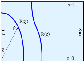
Figure 1: We are locating apparent horizons of two types: one, having a spherical topology, is conveniently parametrized by $\rho=R(\chi)$ (plotted here as centered at $(0,0)$), and another, having a cylindrical topology, is parametrized by $r=R(z)$.

In either case we define an outward-pointing spacelike unit normal to the surface $f=0$,

$$s^{\alpha}=\frac{\gamma^{\alpha\beta}\,f_{,\beta}}{\sqrt{\gamma^{\rho\sigma}\,f_{,\rho}\,f_{,\sigma}}}.$$ (35)

The vanishing of the divergence, $\theta$, of the outgoing null rays defined by $l^{\alpha}=s^{\alpha}+n^{\alpha}$ can be expressed as

$$\theta=(\gamma^{\alpha\beta}-s^{\alpha}s^{\beta})\nabla_{\alpha}l_{\beta}=0.$$ (36)

Substituting the expressions (32) or (34) into (36) yields ordinary second order differential equations for $R(\chi)$ or $R(z)$ correspondingly. The equations could be solved by “shooting”, subject to appropriate boundary conditions, however, here we instead use the following point-wise relaxation method, that is more suitable for parallel numerical implementations. We start with supplying an initial guess for the entire function $R$ and iterate the parabolic equation

$$\frac{{\partial}R}{{\partial}\tau}=-\theta(R^{\prime\prime},R^{\prime},R,g_{ab},{\partial}g_{ab},x^{a}),$$ (37)

in unphysical “time” $\tau$ until a solution is found. This equation implies that depending on whether $R(\tau)$ is inside or outside the horizon at any given moment, it will expand or shrink in the next instant. In numerical simulations the hope is that the initial $R$ will “flow” to the apparent horizon in finite time. We find that in our case this indeed happens when the initial guess is “reasonably close” to the final solution.

IV Numerical approach

Here we describe our strategy for the numerical solution of the GH system (with a scalar matter source) in Kaluza-Klein spacetime.

IV.1 The numerical grid and the algorithm

We cover the $t$-$r$-$z$ space by a discrete lattice denoted by $(t^{n},r_{i},z_{j})=(n\,\Delta t,i\,\Delta r,j\,\Delta z)$, where $n,i$ and $j$ are integers and $\Delta t$, $\Delta r$, and $\Delta z$ define the grid spacings in the temporal and two spatial directions, respectively. As described in the next section, the spatial domain is compactified, and hence a grid of finite size $N_{r}\times N_{z}$ extends from the axis to spatial infinity. Approximations to the dynamical fields, collectively denoted here by $Y$, are evaluated at each grid point, yielding the discrete unknowns $Y^{n}_{i,j}\equiv Y(t^{n},r_{i},z_{j})=Y(n\,\Delta t,i\,\Delta r,j\,\Delta z)$. In the interior of the domain, the GH equations and the gauge-driver equations are discretized using ${\cal O}(h^{2})$ finite difference approximations (FDAs), which replace continuous derivatives with the discrete counterparts, examples of which are given in Table 1. As in FP1 ; FP2 ; SorkinChoptuik our scheme directly integrates the second-order-in-time equations.

	Centered derivatives
${\partial}_{t}Y$	$(Y^{n+1}_{i,j}-Y^{n-1}_{i,j})/(2\Delta t)$
${\partial}_{r}Y$	$(Y^{n}_{i+1,j}-Y^{n}_{i-1,j})/(2\Delta r)$
${\partial}_{t}^{2}Y$	($Y^{n+1}_{i,j}-2\,Y^{n}_{i,j}+Y^{n-1}_{i,j})/(\Delta t)^{2}$
${\partial}_{r}^{2}Y$	($Y^{n}_{i+1,j}-2\,Y^{n}_{i,j}+Y^{n}_{i-1,j})/(\Delta r)^{2}$
${\partial}_{tr}^{2}Y$	($Y^{n+1}_{i+1,j}-Y^{n+1}_{i-1,j}-Y^{n-1}_{i+1,j}+Y^{n-1}_{i-1,j})/(4\,\Delta t\Delta r)$
${\partial}_{rz}^{2}Y$	($Y^{n}_{i+1,j+1}-Y^{n}_{i-1,j+1}-Y^{n}_{i+1,j-1}+Y^{n}_{i-1,j-1})/(4\Delta r\Delta z)$
	Backward derivatives
${\partial}_{r}Y$	$(4\,Y^{n}_{i+1,j}-3\,Y^{n}_{i,j}+Y^{n}_{i+2,j})/(2\Delta r)$
${\partial}_{r}^{2}Y$	$(2\,Y_{i,j}^{n}-5\,Y_{i+1,j}^{n}+4\,Y_{i+2,j}^{n}-Y_{i+3,j}^{n})/(\Delta r)^{2}$

Table 1: Examples of second order finite-differencing approximation to derivatives calculated at a grid point $(n,i,j)$ that we use in our discretization scheme in the interior of the domain (centered stencil), and at the excision boundary (backward stencil) of the numerical grid.

Following discretization, we thus obtain finite difference equations at every mesh point for each dynamical variable. Denoting any single such equation as

$${\cal L}_{Y}|^{n}_{i,j}=0.$$ (38)

we then iteratively solve the entire system of algebraic equations as follows.

First, we note that for those variables that are governed by equations of motion that are second order in time, our ${\cal O}(h^{2})$ discretization of the equations of motion results in a three level scheme which couples advanced-time unknowns at $t^{n+1}$ to known values at retarded times $t^{n}$ and $t^{n-1}$. In order to determine the advanced-time values for such variables, we employ a point-wise Newton-Gauss-Seidel scheme: starting with a guess for $Y^{n+1}_{i,j}$ (typically, we take $Y^{n+1}_{i,j}=Y^{n}_{i,j}$) we update the unknown using

$${Y^{n+1}_{i,j}}\rightarrow{Y^{n+1}_{i,j}}-{{\cal R}_{Y}|^{n}_{i,j}\over{\cal J}_{Y}|^{n}_{i,j}}.$$ (39)

Here, ${\cal R}_{Y}$ is the residual of the finite-difference equation (38), evaluated using the current approximation to $Y^{n+1}_{i,j}$, and the diagonal Jacobian element is defined by

$${\cal J}_{Y}|^{n}_{i,j}\equiv\frac{{\partial}{\cal L}_{Y}|^{n}_{i,j}}{{\partial}Y^{n+1}_{i,j}}.$$ (40)

In the cases where we used gauge drivers (III.3) we found that an iteration based on the Crank-Nicholson discretization scheme of the corresponding first order equations performed well. Specifically, writing any such equation schematically as $\dot{Y}=f_{Y}(Y,{\partial}Y,\dots)$, we update using

$$Y^{n+1}_{i,j}\rightarrow Y^{n}_{i,j}+{1\over 2}\Delta t\,\left(f_{Y}|^{n+1}_{i,j}+f_{Y}|^{n}_{i,j}\right).$$ (41)

We iterate (39) and (41) over all equations until the total residual norm, see (49), falls below a desired threshold.

In order to inhibit high-frequency instabilities which often plague FDA equations, our scheme incorporates explicit numerical dissipation of the Kreiss-Oliger (KO) type KO . Following FP1 , at the interior grid points, $\{(i,j)|~{}2\leq i\leq N_{r}-2,~{}2\leq j\leq N_{z}-2\}$, and for each dynamical variable we apply a low-pass KO filter by making the replacement

$$Y_{i,j}\to Y_{i,j}-\epsilon_{\rm KO}\,d_{i,j}$$

$$d_{i,j}\equiv \frac{1}{16}\Big{(}Y_{i-2,j}-4\,Y_{i-1,j}-4\,Y_{i+1,j}+Y_{i+2,j}+$$ (42)

$$~{}~{}+Y_{i,j-2}-4\,Y_{i,j-1}-4\,Y_{i,j+1}+Y_{i,j+2}+$$

$$~{}~{}+12\,Y_{i,j}\Big{)}$$

at both the $t^{n-1}$ and $t^{n}$ time-levels before updating the $t^{n+1}$ unknowns. Here $\epsilon_{\rm KO}$ is a positive parameter satisfying $0\leq\epsilon_{\rm KO}\leq 1$ that controls the amount of dissipation. An extension of the dissipation to the boundaries FP1 was also tried, but this has not resulted in any significant improvement of the performance of the code.

IV.2 Coordinates and boundary conditions

While the physical, asymptotically flat (times a circle, in our case) spacetime extends to spatial infinity, in a numerical code one can only use grids of finite size. Instead of using a standard strategy that deals with this issue by introducing an outer boundary at some finite radius where approximate boundary conditions are imposed, we adopt another technique—proven successful in previous work in numerical relativity, see e.g. FP2 ; SorkinChoptuik ; Choptuik_BS —and compactify the spatial domain. We find that compactifying the radial direction and imposing the (exact) Dirichlet conditions (19) at the edge of the domain works well, provided that we use sufficient dissipation. In particular, it is known that due to the loss of resolution near the compactified outer boundary (assuming a fixed mesh spacing in the compactified coordinates), outgoing waves generated by the dynamics in the interior will be partially reflected as they propagate toward the edge of the computational domain, and these reflections will then tend to corrupt the interior solution. By adding sufficient dissipation one can damp the waves in the outer region, attenuating any unphysical influx of radiation. This enables one to use the compactification meaningfully.

The results presented in this paper were obtained using the compactification of the form

$$\tilde{r}=\frac{r}{1+r},$$ (43)

where the compactified $\tilde{r}$ ranges from $0$ to $1$ for values of the original radial coordinate $r\in[0,\infty)$. In practice, we define a uniform grid in the compactified $\tilde{r}$ and use chain-rule to replace derivatives with respect to $r$ with the derivatives with respect to $\tilde{r}$ in all dynamical equations. The asymptotic boundary conditions (19) at $\tilde{r}=1$ are then imposed exactly: $g_{ab}=\eta^{(3)}_{ab},\lambda=0,\Phi=0$, and $H_{a}=W_{a}=0$.

We have previously described the boundary (regularity) conditions at $\tilde{r}=r=0$ in Sec. III.1. Denoting by $Y^{n+1}_{1,j}$, for $j=2,\dots,N_{z}-1$, the advanced-time value at the axis for any of the variables, $g_{00},g_{11},g_{22},g_{02}$,$H_{0}$, and $H_{2}$ that have vanishing derivative at $r=0$, we use the update $Y^{n+1}_{1,j}=(4\,Y^{n+1}_{2,j}-Y^{n+1}_{3,j})/3$, which is based on a second-order backwards difference approximation (see Table  1) of $\partial_{r}Y=\partial_{\tilde{r}}Y=0$. For the quantities $g_{01},g_{12},\lambda$ and $H_{1}$, which are odd in $r$ as $r\to 0$, we simply use $Y^{n+1}_{1,j}=0$.

For simplicity, in this paper we consider only configurations that have reflection symmetry about $z=0$ which together with periodicity in z, implies

$${\partial}_{z}Y|_{z=0}={\partial}_{z}Y|_{z=L}=0.$$ (44)

We update points at $z=0$ and $z=L$ using backward difference approximation similar to that in Tab. 1. In particular for $i=2,\dots,N_{r}-1$, we use $Y^{n+1}_{i,1}=(4\,Y^{n+1}_{i,2}-Y^{n+1}_{i,3})/3$ at $z=0$, and $Y^{n+1}_{i,N_{z}}=(4\,Y^{n+1}_{i,Nz-1}-Y^{n+1}_{i,Nz-2})/3$ at $z=L$.

IV.3 The elliptic equation of initial data

It turns out that generally the equation (III.4) for the conformal factor is ill-posed, namely that the linear equation governing small perturbations about a solution of (III.4) does not admit a unique solution for given boundary conditions York . Therefore, an attempt to solve (III.4) using standard relaxation methods will generically fail, as the relaxation is not guaranteed to converge. However, a method circumventing this difficulty exists York , and this is through a rescaling $\Phi=\hat{\Phi}\,\psi^{s}$ that transforms the Hamiltonian constraint (III.4) into

$${\partial}_{r}^{2}\psi+{\partial}_{z}^{2}\psi+\frac{n}{r}{\partial}_{r}\psi+\frac{n-1}{\psi}\left[({\partial}_{r}\psi)^{2}+({\partial}_{z}\psi)^{2}\right]+$$

$$\frac{s^{2}\psi^{2\,(s-1/2)}}{4(n+1)}|\hat{\Phi}|^{2}\left[({\partial}_{r}\psi)^{2}+({\partial}_{z}\psi)^{2}\right]+$$

$$\frac{s\psi^{2\,s}}{4(n+1)}\left({\partial}_{r}|\hat{\Phi}|^{2}{\partial}_{r}\psi+{\partial}_{z}|\hat{\Phi}|^{2}{\partial}_{z}\psi\right)+$$ (45)

$$\frac{\psi^{2\,(s+1/2)}}{4\,(n+1)}\left(|{\partial}_{r}\hat{\Phi}|^{2}+|{\partial}_{z}\hat{\Phi}|^{2}\right)+$$

$$\frac{\omega^{2}\psi^{2\,(s-2\,n+5/2)}}{4\,(n+1)}|\hat{\Phi}|^{2}+\frac{\psi^{5}}{2\,(n+1)}\,V(|\Phi|\,\psi^{s})=0.$$

By choosing the power $s$ such that terms in this equation which are proportional to $\psi^{p_{i}}$ have only non positive $p_{i}$’s one renders the problem well posed York . In the case of a free scalar field having the potential $V\propto|\Phi|^{2}$, which we assume here, this implies that $s<-5/2$, see a related discussion in SorkinPiran .

Note that the physical data are $\Phi$, not ${\hat{\Phi}}$, and therefore we solve equation (IV.3) in an iterative manner where we start with an initial guess $\psi=\psi_{0}(r,z)$ and at each iteration $i>1$ update ${\hat{\Phi}}_{i+1}=\Phi\,\psi_{i}^{-s}$ that is then used in (IV.3) in order to solve for $\psi_{i+1}$. Most of the results obtained in this paper were generated using $\psi_{0}=1$ and $s=-3$. Interestingly, it turns out that provided the initial guess is not too distant from the solution, the original equation (III.4) is numerically stable without the rescaling. This happens, for instance, in the weak field regime where the guess $\Psi_{0}=1$ relaxes to the solution without any trouble.

IV.4 Excision

We use excision to dynamically exclude from the computational domain a region interior to the apparent horizon that would eventually contain the black hole singularity. This approach relies on the observation that in spacetimes that satisfy the null energy condition and assuming the cosmic censorship holds, the apparent horizon is contained within the event horizon. This ensures that the excluded region is causally disconnected from the rest of the domain (see thornburg_excision and the references therein for further discussion). Operationally, once an apparent horizon is found, we introduce an excision surface, $R_{\rm EX}$, contained within the apparent horizon, and such that all characteristics at $R=R_{\rm EX}$ are pointing inwards. This specific characteristic structure eliminates the need for boundary conditions at $R_{\rm EX}$: rather, advanced-time unknowns located on the excision surface are computed using finite difference approximations to the interior evolution equations, but where centered difference formulas are replaced with the appropriate one-sided expressions given in Table 1.

Currently our apparent horizon finder is only capable of locating horizons of the shapes depicted in Fig. 1. In this case the radius of the excision surface typically satisfies $R_{\rm EX}\raisebox{-2.15277pt}{$\>\stackrel{{\scriptstyle\textstyle<}}{{\sim}}\>$}0.7R_{\rm AH}$, where $R$ is the coordinate radius.

V Performance of the code

In this section we investigate the performance of the code in series of simulations that evolve regular initial distribution of complex scalar field in five and six dimensional Kaluza-Klein spacetime. The code uses pamr/amrd infrastructure pamr_amrd where our suitably interfaced numerical routines are called by the amrd driver. All our results are generated using an initial scalar field profile of the Gaussian form (24), with fixed values $r_{0}=z_{0}=0$ and $\Delta=0.25$, so that the scalar pulse is always initially centered at the axis, see Fig. 2.

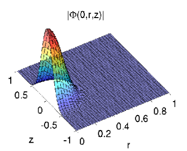
Figure 2: We choose the initial distribution of the scalar field as a generalized Gaussian (24) and assume that the initial time derivative is given by (25). We mostly consider localized initial pulses (such as the one shown here), that are obtained by setting $e_{r}=e_{z}=0$ in (24). The radial direction is compactified, and the hypersurfaces $z=1$ and $z=-1$ identified in a Kaluza-Klein spacetime under consideration.

In addition, we set $e_{r}=0$ and use $e_{z}=0$, unless otherwise specified. We choose the initial frequency in (25) to be $\omega=20$, and the asymptotic size of the KK circle, ${\hat{L}}=2$. The scalar field potential used here is taken to be of the form $V(\Phi)=m_{\Phi}^{2}\,|\Phi|^{2}$, where without much loss of generality we set $m_{\Phi}=1$.

Because we mostly use a time-explicit finite difference scheme, we expect restrictions on the ratio $\lambda_{C}\equiv\Delta t/h$ (the Courant factor) that can be used while maintaining numerical stability. In the results discussed below we chose $0.2\lesssim\lambda_{C}\lesssim 0.5$ in the weak-field regime, and $0.05\lesssim\lambda_{C}\lesssim 0.25$ for evolving the strong data. Taking larger $\lambda_{C}$ usually leads to amplification and dominance of numerical errors near the axis, that shows up as diverging high frequency oscillations. In most cases we use uniform grids of the same size in both spatial directions, $h\equiv\Delta r=\Delta z$, and our lowest and highest resolution simulations have $h=1/16$ and $h=1/256$, respectively. The highest-resolution runs generally required $\lambda_{C}\leq 0.2$ for stability.

As expected, the outcome of the collapse depends on the strength of the initial data. Low density distributions describe weakly gravitating scalar pulses which completely disperse in all instances. Strong data generate spacetimes in which black holes form, or almost form. For fixed $\Delta,e_{r},e_{z},m_{\phi},{\hat{L}}$ and $\omega$ a single free parameter that controls the strength of the pulse—and hence, the outcome of the evolution—is the initial amplitude $\Phi_{0}$. In this case “strong initial data” will refer to situations when an increase of the initial amplitude by less than $10\%$ leads to formation of a curvature singularity, and the other data will be called “weak”. The critical amplitude is at the threshold for the singularity formation.

For each spacetime that we construct, the asymptotic mass and tension are computed using (31), where the constants $a$ and $b$ are found by fitting the metric components $g_{tt}$ and $g_{zz}$ with the functions of the form $g(r)=g_{\infty}+g_{1}/r^{n}+g_{2}/r^{n+1}$ in the asymptotic region. The errors in the constants are determined by the fitting uncertainty which in our case is $\sim 1-2\%$ (larger for weaker data). We find that our initial data sets usually have $a\simeq n\,b$, and it follows from (31) that $\tau\simeq 0$, within the numerical accuracy of our method.

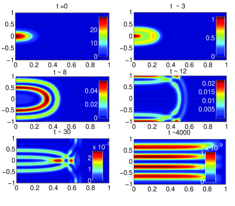
Figure 3: Snapshots of the evolution of energy-momentum density $\rho=n^{a}\,n^{b}\,T_{ab}$ in the simulation of the initial data defined by $\Phi_{0}=0.35\,(1-i)$ in 5D, using algebraic DWG. The horizontal axis represents the compactified radial direction, and the vertical axis is along the periodic $z$-direction. The lapse of time is measured in units of the total mass. The initial collapse of the pulse around the center $(r,z)=(0,0)$ is accompanied by a growth of the amplitude of $\rho$ by about an order of magnitude. The pulse then bounces off and several outgoing shells form. The shells propagate along the periodic $z$-direction and interact, creating a typical interference pattern. As expected, the $z$-dependence vanishes in the asymptotic regions. In the later stages of the evolution $\rho$ is small, and the frequency spectrum of the oscillations along $z$ is dominated by a few lowest eigenfrequencies associated with the compact KK circle.

A useful quantity that illustrates energy-momentum distribution is the density $\rho=T_{ab}n^{a}n^{b}$. Figure 3 depicts $\rho$ at several moments during the 5D evolution of weak initial data defined by $\Phi_{0}=0.35\,(1-i)$, using algebraic damped wave gauge (DWG), see (20). Figure 3 shows that in the early stages of the evolution the pulse (initially localized around the center $(r,z)=(0,0)$) undergoes a gravitational collapse that is accompanied by a growth of the central energy-density. At a later time, however, the pulse bounces off while forming several shells, and disperses. The distribution of the energy density is anisotropic inside the shells, with a higher concentration of energy occurring along the axis, $r=0$, and at the equator, $z=0$. The matter waves that travel along the compact KK circle collide to form a typical interference picture (see Fig. 3) and the pattern becomes increasingly complicated in the course of time, when more and more waves undergo interaction. As expected in the KK background the $z$-dependence of solutions vanishes in the asymptotic region, since the $z$-dependent modes are massive and fall off exponentially fast.

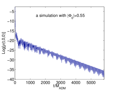
Figure 4: The logarithm of the central energy-density, $\rho$, in a five-dimensional weak field simulation defined by $|\Phi_{0}|=0.55$ that uses algebraic DWG. The resulting spacetime has the mass $M=0.67\pm 0.03$ and the tension is zero within the numerical accuracy. In the early stages of the evolution, the pulse collapses and $\rho$ grows. Subsequently, the energy density decreases following a power-law dependence during the period lasting from $t\sim{\cal O}(10)M$ until $t\sim{\cal O}(100)M$. After that $\rho$ decays exponentially $~{}\exp[-t/(800M)]$. The high-frequency oscillations are associated with the eigenmodes of the compact KK circle.

In order to obtain more quantitative insight into the process, we plot in Fig. 4 the evolution of the logarithm of $\rho$ at the center. During the highly dynamical early epoch, lasting until $\sim{\cal O}(10)M$, the field collapses, bounces off the center, spreads along the $z$-direction, and starts dispersing to infinity. In the first stage of the dispersion, lasting until $\sim{\cal O}(100)M$, the decay of $\rho$ follows a power-law, and in the late times the decay is exponential with a characteristic time scale of a few hundreds of $M$. The maximal scalar curvature is attained during the initial collapse phase; in the shown simulation the curvature reaches the magnitude of order of $\sim{\cal O}(100)$ (in units of $M^{-2}$). The discrete spectrum of the high-frequency oscillations consists of the normal frequencies $f_{n}\sim n/L,~{}n=1,2,\dots$ defined by the size of the KK circle. We observe that the higher frequency modes decay faster, and the late-time spectrum is dominated by a few lowest frequency modes, see also bottom right panel of Fig. 3.

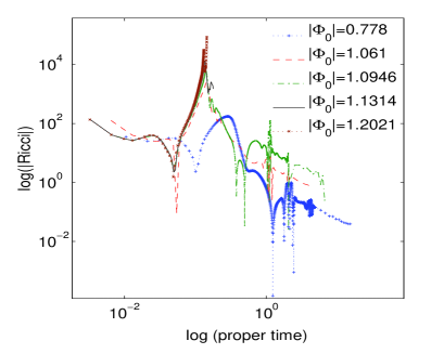
Figure 5: A log-log plot of the Ricci scalar (in units of $M^{-2}$) as a function of the proper time, $t_{\rm prop}\equiv\int_{0}^{t}\alpha\,dt$, both evaluated at the center, in several simulations in $5D$. The first peak in the curves corresponds to the initial collapse phase, and for stronger data the Ricci scalar diverges in finite time, signaling a curvature singularity (case $|\Phi_{0}|=1.2021$). In subcritical cases, the curvature decreases after the initial growth, and the secondary peaks correspond to collisions of the shells traveling along the KK circle and arriving back at $(0,0)$.

When the initial amplitude of the scalar field increases, the maximal curvature achieved during the collapse grows, and when $|\Phi_{0}|$ surpasses a certain threshold, the curvature diverges, signaling the appearance of a singularity; see Fig. 5. Currently we are able to estimate the critical amplitude with a relatively low precession of approximately 1 part in 800. In five dimensions the amplitude is between $1.0946$ and $1.096$ such that initial data with $|\Phi_{0}|\leq 1.0946$ completely disperses, and the data $|\Phi_{0}|\geq 1.096$ gives rise to curvature singularities and black holes.

A covariant way to illustrate the distribution of matter and the geometry of the spacetime is provided by the Ricci scalar, and Fig. 6 shows its evolution computed in the evolution of our strongest subcritical data set, $|\Phi_{0}|=|0.774(1-i)|\simeq 1.0946$. The initial pulse collapses, bounces off and forms several shells, that start dispersing after $t\sim 0.2M$. While the anisotropy of the energy distribution inside the shells is small for weak data, it is obvious in the strong field regime. Some matter is ejected along the equator, $z=0$, and two distinctive pulses, moving in the opposite directions, form at the axis. The pulses collide and interact, which results in smearing of the energy-density along the axis, see bottom right panel of Fig. 6. The distribution is not stationary, rather the matter is continuously leaking to infinity, and the late-time behavior is qualitatively similar to the weak field case, shown in Fig. 3.

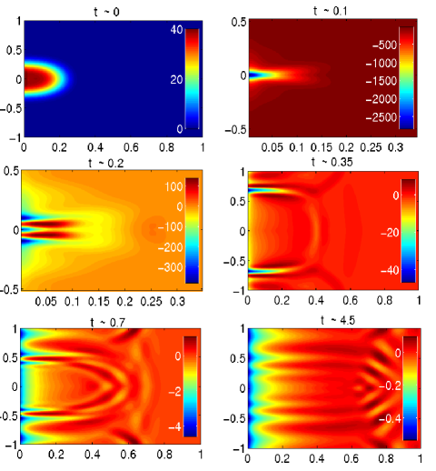
Figure 6: The Ricci scalar at several instants of the evolution of the initial data characterized by $\Phi_{0}=0.774(1-i)$, currently our strongest subcritical data set. The numerical resolution used in this simulation is $129\times 129$. After the initial collapse stage an expanding shell of matter forms. The energy-density distribution inside the shell quickly becomes anisotropic with most of the energy localized within individual pulses traveling along the axis and inside the pulse emitted radially along the equator, $z=0$. The pulses at the axis undergo interactions and spread the energy-density along $r=0$. In late stages of the evolution, all the matter is radiated away to infinity.

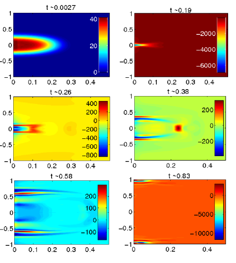
Figure 7: Snapshots of the Ricci scalar at several instants of the evolution of the initial data characterized by $\Phi_{0}=0.775(1-i)$ at the resolution of $257\times 257$. The matter distributes anisoropically inside the bouncing shells such that two localized pulses, traveling along the axis, form. When the pulses collide at $z=1$ a curvature singularity appears.

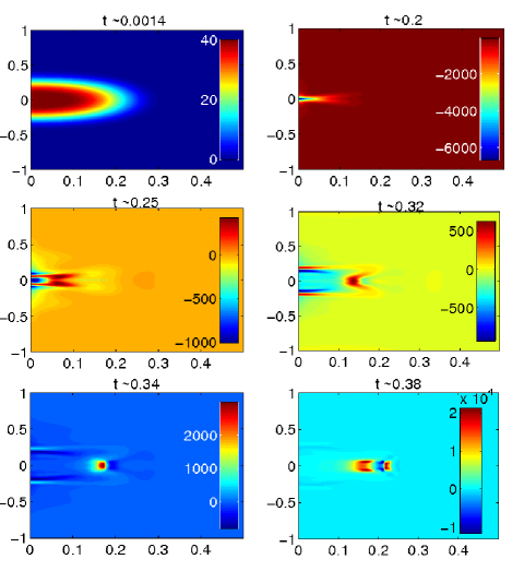
Figure 8: The Ricci scalar at several instants during the evolution defined by $\Phi_{0}=0.777(1-i)$. A curvature singularity forms along the equator, inside the lump of matter emitted in the radial direction during the initial collapse-bounce process. This simulation uses the resolution of $257\times 257$.

It turns out that for higher initial amplitudes, $|\Phi_{0}|\raisebox{-2.15277pt}{$\>\stackrel{{\scriptstyle\textstyle>}}{{\sim}}\>$}1.096$, the pulses that form at the axis are able to individually collapse and develop curvature singularities, indicated by diverging scalar curvature and energy-momentum density while the lapse remains finite (of order one) everywhere. Presently, our horizon-finder is not designed to locate the moving apparent horizons that may arise in this case around the singularities, and it would be very interesting to verify whether or not such engulfing horizons indeed form. The time when the curvature singularities appear depends on the strength of the initial data in the manner that the closer to threshold we are the later into the evolution the curvature diverges. For instance, in the case of $|\Phi_{0}|=1.096$ the pulses, collapse and become singular as they cross the circle and collide at $z\simeq 1$, see Fig 7. However, for $|\Phi_{0}|=1.0975$, the curvature inside each pulse blows up earlier, when they reach $z\sim 1/2$.

Intriguingly, we observe that for even stronger initial data formation of the curvature singularity ensues differently. Specifically, the pulse of matter which is usually emitted during the initial collapse-bounce stage outwards along the equator, is now seen to also be able to collapse and develop a singularity. Snapshots of the process are shown in Fig. 8 that was obtained in the evolution of the data defined by $|\Phi_{0}|=1.099$. Since all our attempts to detect an apparent horizon, engulfing the singular region and the center, have failed we believe that the horizon, if it forms in this case, must be localized around the moving curvature singularity.

In Fig. 9 we plot the Ricci scalar along the equator at $t\sim 0.37M$, shortly before the appearance of a singularity at ${\tilde{r}}\sim 0.21$ causes the code to break down. Figure 9 shows that the maximal value of the Ricci scalar along this slice is determined by the numerical resolution: the finer meshes we use, the larger the values attained. This signals emergence of a curvature rather than a coordinate singularity.

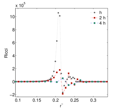
Figure 9: The Ricci scalar (in units of $M^{-2}$) along the equator at $t\sim 0.37M$, shortly before the evolution defined by $\Phi_{0}=0.777(1-i)$ develops a singularity at ${\tilde{r}}\sim 0.21$. The maximal value that the Ricci scalar attains in this evolution depends on the resolution (here $h=1/256$), being larger on finer numerical meshes, which indicates the geometrical nature of the emerging singularity.

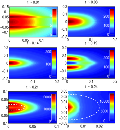
Figure 10: The distribution of energy-density in the evolution of the initial data, defined by $\Phi_{0}=0.8\,(1-i)$ in a simulation that uses the resolution of $201\times 201$ . A strong gravitational interaction in this case precludes any significant amount of matter from escaping to infinity and leads to formation of a black hole soon after the first bounce. The black hole is centered around $(0,0)$ and is signaled by the appearance of an apparent horizon (designated by a thick dashed line) and an explosive growth of the scalar curvature and the energy-density.

Figure 10 shows snapshots of the energy-density distribution obtained in a supercritical simulation initiated by $\Phi_{0}=0.8(1-i)$. The resulting spacetime has the total mass $M=2.40\pm 0.06$ and the tension $\tau\simeq 0$. The initial stages of this evolution are qualitatively similar to those of weaker data, however, after the first bounce off the center (at $t\simeq 0.19M$) the pulse recollapses and a black hole forms as indicated by the appearance of an apparent horizon. The energy-density $\rho$ and scalar curvature both blow up in the vicinity of $(r,z)=(0,0)$ in finite time, while the lapse and shift remain finite.

In order to locate apparent horizons we solve (37) iteratively starting with some initial guess for the entire function that parametrizes the horizon. In the case of $\Phi=0.8(1-i)$ we are searching for a horizon that has spherical topology. We use the parametrization (32) with $r_{0}=z_{0}=0$ and solve (37) initialized by $R=0.1$. Setting the target accuracy to $\sim 10^{-3}$ and using $100$ grid points to represent the horizon, we are able to solve the equation in $\sim 1000$ iterations. The resulting horizon is shown in bottom panels in Fig. 10.

After an apparent horizon is found we use excision to remove a region inside the horizon that contains curvature singularity. However, it turns out that regardless of our specific gauge choice the lapse keeps evolving inside the horizon, and continuously decreases until it is reaching the magnitudes of order $\sim 10^{-5}$ near the excision boundary. In this situation truncation errors in quantities near $R_{EX}$ occasionally cause the computation of non-positive values for the lapse, which immediately leads to code failure. Unfortunately, this happens when the apparent horizon is still fairly dynamical and continues to change its shape and size. Therefore, we are currently not able to determine the stationary black hole state in the end of the evolution.

Figure 11: Distributions of the energy-density (on the right) and the Ricci scalar (on the left) computed in the evolution of a nearly uniform along $z$ initial data defined by $\Phi_{0}=1.2\,(1-i)$, and $e_{r}=0,e_{z}=0.995$, that uses the resolution of $101\times 33$. A strong gravitational interaction leads to a rapid formation of a black string, signaled by the appearance of an apparent horizon of cylindrical topology (shown as a thick dashed line). Note, that the matter and the curvature inside the horizon are strongly localized around the center $r=z=0$.

Having described the low mass configurations we will now briefly discuss more massive solutions of certain type. One initial configuration that we have evolved consisted of a nearly uniform along $z$ distribution of the matter—achieved by setting $e_{z}=0.995$ in (24)—with the initial amplitude of $\Phi_{0}=1.2(1-i)$. The Ricci scalar and the energy-density computed in this evolution are shown in Fig. 11 together with the resulting apparent horizon that appears at $t\sim 0.55$ and has a cylindrical topology. In this simulation we used the algebraic DWG condition, and in this case we were not able to locate a surface on which all characteristics will point inwards. Therefore, no excision was employed in this evolution, and the eventual failure of the code was caused by collapse of the lapse at the axis.

While the total mass of this spacetime, $M\simeq 24.5$, is determined by the asymptotic fall-off (31), the mass of the “black string” (a black hole with the smeared horizon) can be estimated from the average size of its horizon. The last moment of the evolution before the code had crashed is shown in bottom panels of Fig. 11. The horizon is nearly uniform along $z$ and is located at ${\tilde{r}}_{AH}\sim 0.3$, which yields the mass of $M_{BS}=0.5R_{AH}/(G_{N}/{\hat{L}})\simeq 12$, where $R_{AH}\sim 0.49$ is the uncompactified average areal radius of the horizon. This value is below the critical mass, $M_{c}\simeq 14$, needed for stability of the extended solutions of this type GL . Therefore, at this stage the system is probably far from approaching stationarity. Since the total available mass is higher than $M_{c}$ several scenarios for subsequent dynamics can be imagined. If the black hole accretes enough matter and increases its mass above critical, it can reach the uniform black-string end-state. Otherwise, the evolution would probably have to proceed via forming a localized black hole in the first place. This black hole then may or may not accrete additional matter, and as a result either to grow and become a black string or to settle down to a stationary solution of spherical topology. While further investigation of the process is clearly needed, Fig. 11 shows a developing progressive localization of energy-density and curvature around $(0,0)$, indicating that formation of a localized black hole first is more probable in this specific case.

We turn now to a detailed description of the performance of the code. Since we have implemented a free evolution scheme, we can assess the convergence of our numerical solutions by monitoring discrete versions of the Hamiltonian and momentum constraints, which are defined by contracting the Einstein equations with the unit normal vector to the $t={\rm const}$ hypersurfaces, i.e. $M_{a}\equiv n^{a}(G_{ab}-T_{ab})$, where $G_{ab}$ is the Einstein tensor. One way of doing this involves evaluation of the following $L_{2}$-norm of finite-differencing variables

$$\|Y\|_{L_{2}}={\left(\frac{1}{N_{r}\,N_{z}}\sum_{i,j=1}^{N_{r},N_{z}}|Y_{i,j}|^{2}\right)^{1/2}},$$ (46)

In the next section, we compute the $L_{2}$-norms of the constraints at each time step and examine their behavior as a function of various parameters of the problem.

V.1 Coordinate conditions

In the weak-gravity regime where an initial pulse of matter completely disperses to infinity we find clear advantage of the algebraic DWG conditions. They are robust, almost do not require fine-tuning, and are extremely stable. Additionally, as described in the next section, the constraints remain well preserved in this case, such that only very small damping (controlled by the parameter $\kappa$, see (9)) needs to be added to the equations.

Since at $t=0$, we assume harmonic conditions $H_{a}=0$, choosing the source functions according to (20) at $t>0$ will create discontinuity in the temporal component of the gauge source function. Therefore, we multiply the sources $F_{a}$ in (20) by a time-dependent function $(1-\exp(-t/t_{0}))(1+s\exp(-t/t_{1}))$, where $t_{0},t_{1}$, and $s$ are parameters. While the first factor is used to gradually turn the sources on, the second factor is introduced in order to improve late time stability. For instance, while we found that weak data defined by $|\Phi_{0}|\raisebox{-2.15277pt}{$\>\stackrel{{\scriptstyle\textstyle<}}{{\sim}}\>$}0.35$ can be simulated using $t_{0}\sim 0-1$ and $s=0$, the parameters $t_{0}\sim 0-0.2$, $s\sim 0.1-0.5$ and $t_{1}\sim 10$ were required in order to maintain regularity during evolution of stronger data. In addition, we found that long-term stability of the strong data evolutions improves when the factor $\exp(n\,S)$ is removed from the definition of the determinant $\gamma=(g_{11}\,g_{22}-g_{12}^{2})^{1/2}\exp(n\,S)$ used in (20).

The simulations that employ algebraic DWG are stable for a range of the parameters $\mu_{1}$ and $\mu_{2}$. Basically, any values of these parameters of order one can be successfully used in the collapse situations. Nevertheless, we still find that certain choices of $\mu_{1,2}$ perform better than others and preserve the constraints with a greater accuracy. This is illustrated in Fig. 12 where we show norms (46) of the constraints as a function of time. Although, the norms decrease in all the instances, the constraints violations are the smallest for $\mu_{1}=\mu_{2}\simeq 2$.

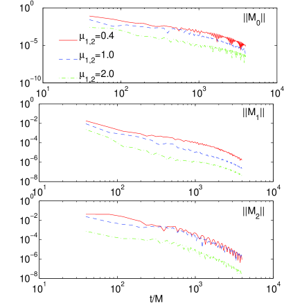
Figure 12: While evolutions are usually stable for any values of order one of the parameters $\mu_{1,2}$ in (20), instabilities develop if these parameters are too small or too large. Here we show the behavior of the norms of the constraints (46) in the simulation of the date defined by $\Phi_{0}=0.3$ in 6D. The evolution is stable for $0.3\raisebox{-2.15277pt}{$\>\stackrel{{\scriptstyle\textstyle<}}{{\sim}}\>$}\mu_{1,2}\raisebox{-2.15277pt}{$\>\stackrel{{\scriptstyle\textstyle<}}{{\sim}}\>$}5$ and the decay rate of the constraint violations is optimized for $\mu_{1,2}\simeq 2$.

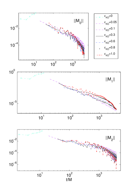
Figure 13: The behavior of the Hamiltonian and the momentum constraints, $M_{a}\equiv n^{a}(G_{ab}-T_{ab})$, as a function of the dissipation parameter $\epsilon_{KO}$ in a 6D simulation with $\Phi_{0}=0.3\,(1-i)$ and the resolution $33\times 33$. While for $\epsilon_{KO}\raisebox{-2.15277pt}{$\>\stackrel{{\scriptstyle\textstyle<}}{{\sim}}\>$}0.04$ the constraints blow up and the code diverges, above this threshold the evolution is stable for arbitrary long periods of time, and any constraint violations decrease in the course of evolution.

After experimenting with the driver version of DWG condition (III.3), we find that it performs comparably to the algebraic DWG in early stages of the evolution until $t\sim 10M$. However, late-time behavior is fairly sensitive to the driver parameters and generically develops coordinate singularities on a timescale $t\sim 30-100M$. A considerable constraint damping was usually required in these cases. In comparison, a DWG-driver simulation with parameters identical to the algebraic DWG evolution shown in Fig. 4, had required at least 50 times stronger damping in order not to diverge immediately, but even then the evolution remained stable only until $t\sim 100M$.

The performance of the gauge drivers (III.3) and (22) is similar to that. It was already reported in SorkinChoptuik that those drivers—known to perform well in Cartesian implementations FP3 ; FP2 —are considerably less stable in spherical symmetry, and here we notice the same. Specifically, we find that pure harmonic coordinates are useful only for simulating the dynamics of very weak initial data with the scalar amplitude $|\Phi_{0}|\raisebox{-2.15277pt}{$\>\stackrel{{\scriptstyle\textstyle<}}{{\sim}}\>$}10^{-3}$ (and the corresponding mass $M\raisebox{-2.15277pt}{$\>\stackrel{{\scriptstyle\textstyle<}}{{\sim}}\>$}10^{-4}$). For larger values of $|\Phi_{0}|$ the lapse function collapses in the locus of maximal matter concentration and coordinate singularity forms. Although we were able to delay the pathology by using of one the drivers (III.3,22), in no instance was it possible to eliminate it completely. Generically, the coordinates in these simulations become singular after a time of approximately a few tens of $M$. An extensive fine-tuning of the driver parameters together with stronger constraint damping and the numerical dissipation enables one to extend somewhat the duration of the regular evolution. up to $t\sim 100M$. For example, a parameter setting that kept the evolution of the $|\Phi_{0}|=0.5$ data regular until $t\sim 100M$ consisted of $\epsilon_{KO}=0.34,~{}\lambda_{C}=0.1,~{}\xi_{1}=0.6,~{}\xi_{2}=0.8,~{}\xi_{3}=0,~{}\alpha_{0}=1,~{}q=3$ and $N_{r}\times N_{z}=41\times 41$.

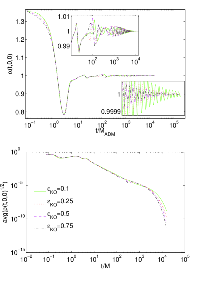
Figure 14: The lapse at the center and the energy-density averaged along the axis are shown as functions of time for various values of $\epsilon_{KO}$ in a subcritical 5D simulation, with $\Phi_{0}=0.4\,(1-i)$. Provided we use sufficient dissipation, ($\epsilon_{KO}>0.08$ in this case), the behavior of dynamical variables is essentially independent of the specific $\epsilon_{KO}$ in early time until $\sim 900\,M$, see the upper inset in the top panel. While at the late times the absolute values of variables in the simulations with stronger dissipation are generically smaller than those in simulations using less dissipation, the variations of the fields are very small at this stage in all instances, see bottom inset.

Our preliminary experiments in supercritical regimes indicate that the algebraic DWG still outperforms the driver conditions. While in all our simulations where a black hole forms the coordinates eventually become singular near the excision surface, the simulations employing algebraic DWG remain stable for longer. It is presently unclear whether the coordinate pathology is caused by the strong gravitational field or by the introduction of the excision surface. More experiments are required and will be reported elsewhere.

V.2 Dissipation and constraint damping

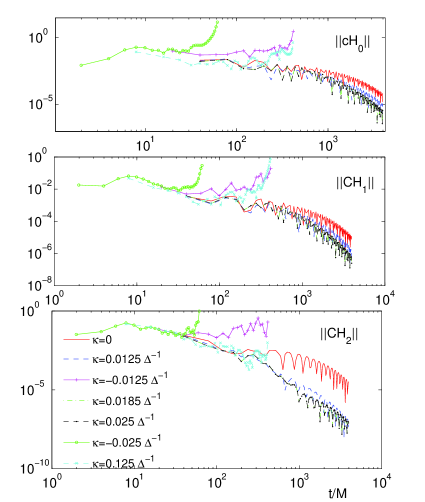
Figure 15: The dynamics of the norm (46) of the GH constraints (5) depends on the amount of the damping. In simulations of the initial data defined by $\Phi(0,r,z)=0.3\,(1-i)\exp[-(r^{2}+z^{2})/0.25^{2}]$ that employ algebraic DWG any constraint violations decrease in time, provided $\kappa\lesssim 0.0185\Delta^{-1}$; for larger values of $\kappa$ the constraint violations diverge. An optimal preservation of the constraints in this case is achieved for $\kappa\simeq 0.05/(1+0.05\,t)$.

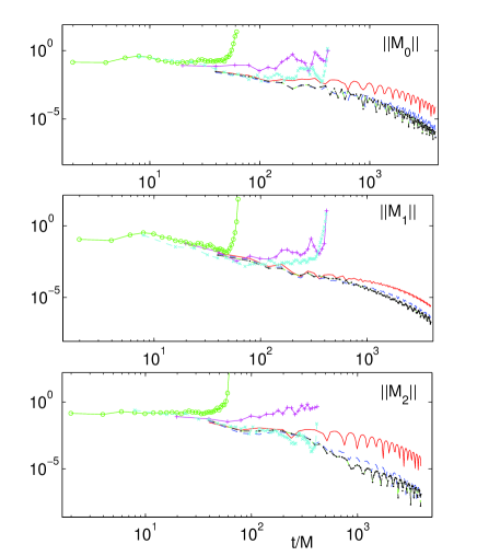
Figure 16: Same simulation and same notations as in Fig.15. The Hamiltonian and the momentum constraints are asymptotically satisfied provided a correct amount of damping is used.

The explicit numerical dissipation that we add to our scheme in (IV.1) is an important ingredient affecting the long-term stability, and Fig. 13 illustrates this. There we fix $\Phi_{0}=0.3\,(1-i)\exp[-(r^{2}+z^{2})/0.25^{2}]$, use resolution of $33\times 33$ and algebraic DWG conditions with $\mu_{1,2}=2$ and $q=1/2$ in a 6D simulation. We find that without the dissipation the constraints quickly diverge. However, for $\epsilon_{KO}$ above a certain minimal value ($\epsilon_{KO}>0.04$ in this case) the evolution stabilizes. The specific threshold value increases slightly when denser grids and stronger initial data are used; however, taking $\epsilon_{KO}\simeq 0.15-0.4$ was usually a safe choice for the simulations described in this paper.

In Fig. 14 we depict the lapse $\alpha(t,0,0)$ and the matter energy-density $\rho(t,0,z)$, averaged along the axis, as functions of time for several choices of $\epsilon_{KO}$ in 5D simulations of weak scalar pulse with $\Phi_{0}=0.4\,(1-i)$ using algebraic DWG. The simulations converge for a wide range of the values of the dissipation parameter, provided $\epsilon_{KO}\raisebox{-2.15277pt}{$\>\stackrel{{\scriptstyle\textstyle>}}{{\sim}}\>$}0.08$. Figure 14 demonstrates that in this case the specific values of $\epsilon_{KO}$ have only a marginal effect on the early dynamics, until approximately $1000\,M$. However, after that time the variables computed in the simulations using unequal dissipation parameters begin to differ, and stronger dissipation generically implies smaller late-time amplitudes. The absolute values of the amplitudes are usually small at this stage (typically below $\sim 10^{-4}$).

Another factor influencing stability is the constraint damping term (9), which we add to the Einstein equations in (10). We find that quite generically the long-term stability improves when the damping of the constraints vanishes in the asymptotic regions. For this reason we multiply $\kappa$ by a factor $(R_{0}/R)$ in the regions where the areal radius satisfies $R>R_{0}$ for some large $R_{0}$ (typically $R_{0}\sim 20$) in order to gradually turn the damping off.

Figures 15 and 16 illustrate the effect of the damping in the case $\Phi(0,r,z)=0.3\,(1-i)\exp[-(r^{2}+z^{2})/0.25^{2}],~{}\epsilon_{KO}=0.5$ in 6D simulations that use algebraic DWG with $\mu_{1,2}=1$ and $q=1/2$, and the resolution of $33\times 33$. In this configuration the evolution is stable for rather small values of $\kappa$ including that of $\kappa=0$; however, the quickest asymptotic decrease of the constraint violations is achieved for $\kappa=0.05/(1+0.05\,t)$. For the values of $\kappa$ greater than a certain value—$\kappa>0.25$ in this specific simulation—the code diverges. The time-dependent factor $1/(1+0.05\,t)$ is less crucial in shorter subcritical simulations, but it helps to improve stability on the long time scales of $t\raisebox{-2.15277pt}{$\>\stackrel{{\scriptstyle\textstyle>}}{{\sim}}\>$}2000\,M$.

Interestingly, typical values of the damping parameter $\kappa$ in algebraic DWG evolution are small compared to the inverse of any typical length scales of the problem (set e.g. by the initial width of the scalar pulse, $\Delta$, by the size of the KK circle or by the size of the black hole). Moreover, certain weaker initial data can even be simulated without the damping at all. This is in sharp contrast to the typical values of the damping parameter, $\kappa~{}\simeq 1/\Delta$, required in simulations that employ the driver gauge conditions (III.3), (III.3), or (22).

V.3 Convergence

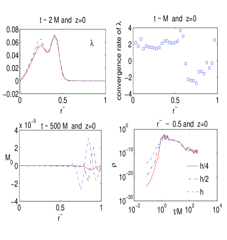
Figure 17: A convergence in a 5D algebraic DWG evolution of $\Phi_{0}=0.4\,(1-i)$, with $h=1/32$. Top panels indicate that in the regions where a non-negligible amount of matter is present the convergence rate (48) of the metric function $\lambda$ is essentially $p\sim 2$. Other functions, such as energy density, depicted in the bottom right panel, have similar convergence trends. The bottom left panel illustrates that the constraint violations consistently decrease with increasing resolution.

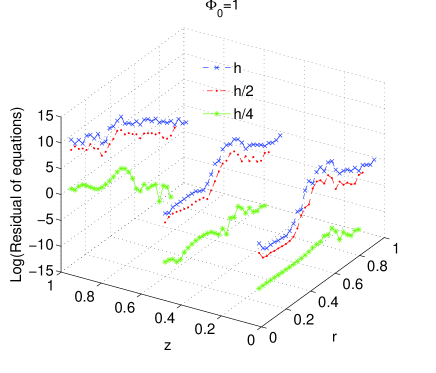
Figure 18: The total residual (49) of the system of our FDA equations at the hypersurfaces $z=0,z=1/2$ and $z=1$ for 3 resolutions, with the coarsest one $h=1/32$. The residual quickly decreases as a function of the numerical resolution.

One of the crucial tests of numerical FDA schemes, such as one that we use here, involves the investigation of the convergence of the generated numerical solutions as a function of resolution. We perform convergence tests based on the assumption Richardson that for any of the unknown functions, $Y(t,r,z)$, appearing in our system, the corresponding discrete quantity, $Y_{h}(t,r,z)$ in the limit $h\to 0$ admits an asymptotic expansion of the form

$$Y_{h}(t,r,z)=Y(t,r,z)+h^{p}e_{p}(t,r,z)+\cdots$$ (47)

where $h$ is the spatial mesh size, $e_{p}(t,r,z)$ is an $h$-independent error function, and $p$ is an integer that defines the order of convergence of the scheme. We consider sequences of three calculations performed with identical initial conditions, but with varying resolutions, $h$, $h/2$ and $h/4$, and compute

$$\log_{2}\left(\frac{Y_{h}-Y_{h/2}}{Y_{h/2}-Y_{h/4}}\right)\approx p,$$ (48)

for a grid function $Y$.

We fix $\Phi_{0}=0.4\,(1-i)$ and use algebraic DWG evolution in 5D with the parameters $\mu_{1,2}=3,q=1/2,\kappa=0.07,\epsilon=0.125$, and show in Fig. 17 several plots illustrating the convergence. The top left panel shows the radial dependence of the metric function $\lambda$ along $z=0$ at $t\sim 2\,M$ obtained in simulations using 3 different resolutions, $h,h/2$ and $h/4$, with $h=1/32$. The decreasing differences between solutions obtained using increasing resolutions indicate convergence. The top right panel in Fig. 17 shows that the convergence rate (48) is mostly quadratic, except in the asymptotic region where the amplitude of the field is small and the computation is unreliable. The bottom left panel depicts the Hamiltonian constraint at a late moment of the evolution: violations of the constraint are small and decrease further when the grid is refined. Finally, the bottom right panel illustrates the time variation of the logarithm of the matter energy-density at $(\tilde{r},z)\sim(0.5,0)$. Again, a convergence is evident and is compatible with $p\raisebox{-2.15277pt}{$\>\stackrel{{\scriptstyle\textstyle>}}{{\sim}}\>$}1.5$ in the regions where a non-negligible amount of matter is present.

An additional measure of accuracy of the scheme can be obtained by monitoring the total normalized residual of our equations that can be defined as

$${\cal R}=\left(\frac{\sum_{i,j=1}^{N_{r},N_{z}}\sum_{Y}|{{\cal R}_{Y}}_{i,j}|^{2}}{{N_{r}\,N_{z}}\,\sum_{Y}1}\right)^{1/2}$$ (49)

where ${{\cal R}_{Y}}_{i,j}$ is the residual of the FDA equation governing the variable $Y$ at a grid-point $(i,j)$. We show the logarithm of the residual in Fig. 18 for three resolutions $h,h/2$ and $h/4$, with $h=1/32$ in the 6D simulation using algebraic DWG and the initial scalar pulse amplitude $\Phi_{0}=1.0\exp(-(r^{2}+z^{2})/0.125)$. Evidently, the residual quickly decreases as a function of the numerical resolution, again indicating convergence of the scheme.

V.4 Conclusion

We have described a generalized harmonic formulation of the Einstein equations in axial symmetry in $D$-dimensions and constructed the first numerical code based on it. We chose the coordinates in which the background symmetries are explicit. This, however, resulted in a coordinate singularity on the axis, $r=0$. While at the continuum level the equations of motion ensure regularity of a solution on the axis, extra care must be exercised so that this remains true in discrete numerical calculations. We have devised a regularization procedure that achieves that, while preserving the hyperbolicity of the evolution system. In our implementation we integrate the full $D$-dimensional equations and find that this approach is smoother at the axis and is generically more stable compared to the approach that solves the 2+1 equations, obtained by a dimensional reduction on the symmetry.

We expect that our new code will enable systematic investigation of many problems of interest in axisymmetry. As a first application we tested the performance of the code in the context of fully nonlinear gravitational collapse of a complex, self-interacting scalar field propagating in a $D$-dimensional Kaluza-Klein spacetime. We assumed spherical symmetry in the $(D-1)$-dimensional noncompact portion of the spacetime, which effectively reduced the problem to 2+1. The scenarios that we have considered ranged from the dispersion of dilute pulses to the collapse of strongly gravitating pulses that lead to black hole formation. One of the aspects of our code was the use of radial compactification which, in conjunction with sufficient Kreiss-Oliger–type dissipation, provided a viable alternative to the truncation of the spatial domain and the use of approximate outer boundary conditions. Another ingredient of our algorithm that in some regimes was vital for long-term stability was the addition of constraint-damping terms to the evolution equations.

We described several strategies to fixing the coordinate freedom that are compatible with the GH approach and experimented with those. Our studies of evolutions using damped wave gauge that was enforced algebraically indicate robustness of this choice, its weak dependence on parameter settings, and stability. On the other hand, our experiments with various drivers—described in detail in Sec. III.3—reveal that in the case of symmetries these drivers are considerably less effective relative to the $3+1$ simulations that use Cartesian coordinates, a conclusion similar to that drawn in SorkinChoptuik . However, it would be interesting to examine performance of the drivers in additional axisymmetric situations, other than collapse.

One can consider several ways to improve the code. Specifically, it seems natural to use hyperboloidal slicing, similar to one suggested in anil , instead of the spatial compactification that we presently employ. We expect this will allow calculating asymptotic quantities and emitted gravity wave with a greater accuracy, and will help to improve late-time stability of the evolution, that is adversely affected by the unphysical radiation caused by the loss of numerical resolution near the outer boundary. One possible extension of our code which will broaden significantly the spectrum of possible axisymmetric configurations accessible with it, would be an addition of rotation. In addition, coupling the gravity dynamics to evolution of more general matter, such as fluid, will enable studying certain situations relevant in astrophysics.

Although the main purpose of this work was to describe the code and test its performance in a non-trivial highly dynamical setting, our preliminary study of collapse in a Kaluza-Klein background indicates rich and distinctive phenomenology, deserving further investigation. Among interesting questions, which will be addressed elsewhere, is determining what classes of initial data lead to formation of black holes of specific topology and constructing a phase diagram of the solutions (see BH-BS for some predictions concerning the diagram). In addition, a detailed investigation of the situation near threshold for black hole formation and classification of possible outcomes is necessary. In particular, in this regime the fields typically oscillate, creating several outgoing shells. We found that the matter distributes anisotropically within the shells, forming separate bounded systems, and that curvature singularities can develop inside those. We expect that the effect will be more pronounced in higher dimensions where many more shells can form near threshold SorkinOren , and since the gravitational field of an isolated system is increasingly localized in higher dimensions, the shells have a greater chance to separately become bounded systems capable of collapsing and forming black holes. It is worth exploring to which extent the expectations are true. However, such a study will require an improved horizon-finder that will be able to locate several moving horizons, and we are working in this direction.

Finally, it would be very interesting to compute the detailed gravitational-wave signal emitted in various regimes. While from the perspective of a four-dimensional observer all our solutions appear spherical that are not expected to emit any gravitational radiation, the waves are certainly produced and carry energy away. The “missing” energy, as it would be seen in 4D, will then provide a circumferential evidence in favour of the extra-dimensions. In addition, the spectrum of the gravitational waves must contain frequencies associated with the length scale of the extra dimensions. Therefore, by measuring the signal directly one can, in principle, probe the dimension and the topology of the spacetime.

Appendix A Dimensionally reduced equations and boundary conditions

Here we describe the approach that uses the Kaluza-Klein reduction of the $D$ dimensional equations on the $O(D-2)$ symmetry and integrates the resulting three-dimensional equations.

The most general $D$-dimensional line element that is invariant under action of the group of rotational symmetries $O(D-2)$ can be written as

$$ds^{2} = e^{2\,\alpha\,{\hat{S}}}ds_{3}^{2}+e^{2\,\beta\,{\hat{S}}}d\Omega_{n}^{2}$$ (50)

$$= e^{2\,\alpha\,{\hat{S}}}g_{ab}^{(3)}dx^{a}dx^{b}+e^{2\,\beta\,{\hat{S}}}d\Omega_{n}^{2},$$

where the metric components are functions of three-dimensional coordinates $x^{a}$ alone, and $\alpha,\beta$ are constants, chosen for convenience below.

We define the conformally rescaled metric $\tilde{g}_{ab}^{(3)}\equiv e^{2\,\alpha\,{\hat{S}}}g_{ab}^{(3)}$ and write the dimensional reduction of the Einstein-Hilbert Lagrangian as

$${\cal L}_{EH} \equiv \sqrt{-g_{D}}R_{D}=$$ (51)

$$= \sqrt{-{\tilde{g}}_{3}}e^{n\,\beta\,{\hat{S}}}\Big{[}{\tilde{R}}_{3}+n(n-1)\,e^{-2\,\beta\,{\hat{S}}}-$$

$$-2\,n\,\beta\,{\tilde{\Box}}\,{\hat{S}}-n(n+1)\,\beta^{2}\,({\tilde{\partial}}\,{\hat{S}})^{2}\Big{]},$$

where derivatives are computed using ${{\tilde{g}}^{(3)ab}}$: ${\tilde{\Box}}\,{\hat{S}}\equiv(-{\tilde{g}}_{3})^{-1/2}{\partial}_{a}\left({{\tilde{g}}^{(3)ab}}\,(-{\tilde{g}}_{3})^{1/2}\,{\partial}_{b}\,{\hat{S}}\right)$, and $\left({\tilde{\partial}}{\hat{S}}\right)^{2}\equiv{{\tilde{g}}^{(3)ab}}{\partial}_{a}{\hat{S}}{\partial}_{b}{\hat{S}}$.

Substituting the non-tilded metric and using the relations between conformally related quantities Wald ,

$${\tilde{R}}_{3} = e^{-2\,\alpha\,{\hat{S}}}\left[R_{3}-4\,\alpha\,\Box\,{\hat{S}}-2\,\alpha^{2}\,({\partial}{\hat{S}})^{2}\right],$$

$${\tilde{\Box}}\,{\hat{S}} = e^{-2\,\alpha\,{\hat{S}}}\left[\alpha\,({\partial}\,{\hat{S}})^{2}+\Box\,{\hat{S}}\right],$$

$$\left({\tilde{\partial}}{\hat{S}}\right)^{2} = e^{-2\,\alpha\,{\hat{S}}}({\partial}{\hat{S}})^{2},$$ (52)

where the derivatives in the right-hand-side are now computed with the non-tilded metric, we arrive at

$$\sqrt{-g_{D}}R_{D} = \sqrt{-g_{3}}e^{(\alpha+n\,\beta){\hat{S}}}\Big{[}R_{3}-(4\alpha+2\,n\,\beta)\Box{\hat{S}}$$ (53)

$$- \left(2\,\alpha^{2}+2\,n\,\alpha\,\beta+n(n+1)\beta^{2}\right)({\partial}{\hat{S}})^{2}+$$

$$n(n-1)\,e^{-2\,\beta\,{\hat{S}}+2\,\alpha\,{\hat{S}}}\Big{]}.$$

By choosing $\alpha=-n\,\beta$, we convert the lower-dimensional action into Einstein-Hilbert form, ${\cal L}=\sqrt{-g_{3}}R_{3}$. Since in this case $\Box{\hat{S}}$ is multiplied by a constant factor, it does not contribute to the equations of motion and can be omitted. In addition, fixing $\beta=[n\,(n+1)]^{-1/2}$ ensures the canonical normalization of the kinetic term of the scalar ${\hat{S}}$. After these manipulations the Lagrangian becomes

$${\cal L}_{EH}=\sqrt{-g_{3}}\left[R_{3}-({\partial}{\hat{S}})^{2}+n(n-1)\,e^{-2\,c_{n}{\hat{S}}}\right],$$ (54)

where we have defined $c_{n}\equiv\sqrt{(n+1)/n}$. This Lagrangian describes three-dimensional gravity coupled to the self interacting scalar field $S$. The components of the original $D$-dimensional metric $g_{\mu\nu}$ (50) are given in terms of the lower-dimensional fields as

$$g^{(D)}_{ab} = e^{-(2/c_{n})\,{\hat{S}}}\,g^{(3)}_{ab},$$

$$g^{(D)}_{\Omega\Omega} = \exp\left[\frac{2}{\sqrt{n(n+1)}}{\hat{S}}\right]\,g_{\Omega}.$$ (55)

A reduction of the matter Lagrangian of our model (2) takes the form

$${\cal L}_{\Phi}={1\over 2}\sqrt{-g_{3}}\left[|{\partial}\Phi|^{2}+2\,V(|\Phi|)\,e^{-(2/c_{n})\,{\hat{S}}}\right],$$ (56)

yielding the total action of the system,

$$S = S_{EH}+S_{\Phi}=$$ (57)

$$- \frac{1}{2}\int\sqrt{-g_{3}}\Big{[}R_{3}-|{\partial}\Phi|^{2}-({\partial}{\hat{S}})^{2}+$$

$$+ n(n-1)\,e^{-2\,c_{n}{\hat{S}}}-2\,V(|\Phi|)\,e^{-(2/c_{n})\,{\hat{S}}}\Big{]},$$

that describes two interacting scalar fields minimally coupled to gravity in three dimensions. Varying the action with respect to the 3-metric and the fields one obtains the equations of motion,

$$R_{ab} = \bar{T}_{ab}\equiv T_{ab}-g_{ab}\,T=$$

$$={\partial}_{(a}\Phi\,{\partial}_{b)}\Phi^{*}+{\partial}_{a}{\hat{S}}\,{\partial}_{b}{\hat{S}}-$$

$$-g_{ab}\left(-2\,V\,e^{-(2/c_{n})\,{\hat{S}}}+n(n-1)e^{-2\,c_{n}{\hat{S}}}\right),$$

$$\Box{\hat{S}} - c_{n}\,n(n-1)e^{-2\,c_{n}\,{\hat{S}}}+\frac{2}{c_{n}}\,V\,e^{-(2/c_{n})\,{\hat{S}}}=0,$$

$$\Box\Phi - \frac{{\partial}V}{{\partial}\Phi^{*}}e^{-(2/c_{n})\,{\hat{S}}}=0.$$ (58)

Next, we bring the Einstein equations in this system into the GH form using the transformations analogous to (5), (7) but applied to the 3-metric, and add a constraint damping term similar to (9). The resulting hyperbolic system is evolved in time.

We are interested in asymptotically Minkowski times a circle, $\mathbb{R}^{D-2,1}\times S^{1}$ solutions of (A), satisfying $g^{(D)}_{ab}\rightarrow\eta_{ab}$, $g^{(D)}_{\Omega\Omega}\rightarrow r^{2}$, and $\Phi\rightarrow 0$. Using (A) we find that asymptotic boundary conditions obeyed by the reduced fields in this case are $g^{(3)}_{ab}\rightarrow\eta_{ab}r^{2\,n}$ and ${\hat{S}}\rightarrow\sqrt{n(n+1)}\log(r)$. Since it is difficult to handle blowing-up conditions of this sort in numerical implementations, we redefine our variables by factoring out this singular behavior: $g_{ab}\rightarrow g_{ab}r^{2\,n}$ and $S=\hat{S}+\sqrt{n(n+1)}\log(r)$. However, as a result of this transformation, the radial component of the GH source functions defined in (4), acquires a term singular at the axis $H_{1}=n/r+\dots$, where ellipses designate regular at $r=0$ terms. This behavior is similar to what happens in the unreduced system and in analogy to that case we regularize the source functions by subtracting off this singular flat-background contribution, see Sec. III.1. The gauge conditions are then applied to the regularized source functions.

Regularity conditions at the center $r=0$ are again analogous to those in the unreduced case. Specifically $g^{(3)}_{00},g^{(3)}_{11},g^{(3)}_{02},g^{(3)}_{22}$ and $S$ are even functions in $r$ as $r\to 0$, while $g^{(3)}_{01}$ and $g^{(3)}_{12}$ are odd. Moreover, requiring the absence of conical singularity at $r=0$ places an additional condition that $g^{(3)}_{11}-\exp(-c_{n}\,S)={\cal O}(r^{2})$ as $r\to 0$. Since it is desirable to have a number of boundary conditions matching the number of dynamical variables, one might consider a regularization similar to (15) that achieves this by defining $\lambda=({g_{11}}-e^{c_{n}\,S})/r$ that behaves as ${\lambda}\sim{\cal O}(r)$ near $r=0$, one than eliminates $S$ from the scheme and uses $\lambda$ as a fundamental variable instead. However, a closer examination of the equation governing $\lambda$ reveals that the regularization does not work in this case because the equation is not automatically regular at $r=0$ as it was in the unreduced approach. Rather the equation contains term proportional to $1/r$, which is regular only if the constraints are explicitly satisfied. Namely, not only the number of boundary conditions exceeds that of the dynamical fields—as it was before the regularization—but now the extra condition is also algebraically more complicated. Hence, instead of introducing $\lambda$ we opted to implement a more straightforward regularization method that maintains $S$ as a fundamental dynamical variable and uses analytical Taylor-series expansion to compute its value near the axis; see SorkinChoptuik for more details.

A comparison of the dimensionally reduced approach and the full $D$-dimensional method described in the main text, shows that both methods perform comparably in the weak-field regime when $M\raisebox{-2.15277pt}{$\>\stackrel{{\scriptstyle\textstyle<}}{{\sim}}\>$}0.5$. However, for stronger initial data the dimensionally-reduced approach is considerably less stable and prone to developing coordinate singularities, regardless of the gauge conditions that we use. We do not fully understand the reason for this, a further investigation is required, and we hope to report on this puzzling issue elsewhere.

References

- (1) F. Pretorius, Phys. Rev. Lett. 95, 121101 (2005)
- (2) F. Pretorius, Class. Quant. Grav. 22, 425 (2005)
- (3) F. Pretorius, Class. Quant. Grav. 23, S529 (2006)
- (4) M. Campanelli, C. O. Lousto, P. Marronetti and Y. Zlochower, Phys. Rev. Lett. 96, 111101 (2006)
- (5) J. G. Baker, J. Centrella, D. I. Choi, M. Koppitz and J. van Meter, Phys. Rev. Lett. 96, 111102 (2006)
- (6) M. Koppitz, D. Pollney, C. Reisswig, L. Rezzolla, J. Thornburg, P. Diener and E. Schnetter, Phys. Rev. Lett. 99, 041102 (2007)
- (7) M. Boyle et al., Phys. Rev. D 76, 124038 (2007)
- (8) D. Garfinkle and G. C. Duncan, Phys. Rev. D 63, 044011 (2001)
- (9) M. W. Choptuik, E. W. Hirschmann, S. L. Liebling and F. Pretorius, Class. Quant. Grav. 20, 1857 (2003)
- (10) O. Rinne, Class. Quant. Grav. 25, 135009 (2008)
- (11) O. Rinne, Class. Quant. Grav. 27, 035014 (2010).
- (12) M. Alcubierre, S. Brandt, B. Bruegmann, D. Holz, E. Seidel, R. Takahashi and J. Thornburg,Int. J. Mod. Phys. D 10, 273 (2001)
- (13) A. M. Abrahams, K. R. Heiderich, S. L. Shapiro and S. A. Teukolsky, Phys. Rev. D 46, 2452 (1992). D. Garfinkle and G. C. Duncan, Phys. Rev. D 63, 044011 (2001),
- (14) A. M. Abrahams and C. R. Evans, Phys. Rev. Lett. 70, 2980 (1993).
- (15) M. W. Choptuik, E. W. Hirschmann, S. L. Liebling and F. Pretorius, Phys. Rev. D 68, 044007 (2003)
- (16) R. Emparan and H. S. Reall, Phys. Rev. Lett. 88, 101101 (2002)
- (17) R. C. Myers and M. J. Perry, Annals Phys. 172, 304 (1986).
- (18) R. Gregory and R. Laflamme, Phys. Rev. Lett. 70, 2837 (1993)
- (19) G. T. Horowitz and K. Maeda, Phys. Rev. Lett. 87, 131301 (2001)
- (20) M. W. Choptuik, L. Lehner, I. Olabarrieta, R. Petryk, F. Pretorius and H. Villegas, Phys. Rev. D 68, 044001 (2003)
- (21) H. Friedrich. Commun. Math. Phys., 100:525-543, 1985
- (22) H. Friedrich, Class. Quant. Grav. 13, 1451 (1996).
- (23) D. Garfinkle,Phys. Rev. D 65, 044029 (2002)
- (24) L. Lindblom, M. A. Scheel, L. E. Kidder, R. Owen and O. Rinne, Class. Quant. Grav. 23, S447 (2006)
- (25) L. Lindblom and B. Szilagyi,arXiv:0904.4873.
- (26) E. Sorkin and M. W. Choptuik, to appear in Gen. Rel. Grav. (2010) arXiv:0908.2500 [gr-qc].
- (27) L. E. Kidder, M. A. Scheel and S. A. Teukolsky, Phys. Rev. D 64, 064017 (2001)
- (28) O. Brodbeck, S. Frittelli, P. Hubner and O. A. Reula, J. Math. Phys. 40, 909 (1999)
- (29) C. Gundlach, J. M. Martin-Garcia, G. Calabrese and I. Hinder, Class. Quant. Grav. 22, 3767 (2005)
- (30) A. Arbona and C. Bona, Comput. Phys. Commun. 118, 229 (1999). M. Alcubierre and J. A. Gonzalez, Comput. Phys. Commun. 167, 76 (2005)
- (31) E. Sorkin and Y. Oren, Phys. Rev. D 71, 124005 (2005).
- (32) M. W. Choptuik and F. Pretorius, arXiv:0908.1780 [gr-qc].
- (33) J. R. van Meter, J. G. Baker, M. Koppitz and D. I. Choi, Phys. Rev. D 73, 124011 (2006)
- (34) M. A. Scheel, M. Boyle, T. Chu, L. E. Kidder, K. D. Matthews and H. P. Pfeiffer, arXiv:0810.1767 [gr-qc].
- (35) L. Lindblom, K. D. Matthews, O. Rinne and M. A. Scheel, arXiv:0711.2084 [gr-qc].
- (36) B. Kol, E. Sorkin and T. Piran, Phys. Rev. D 69, 064031 (2004)
- (37) T. Harmark and N. A. Obers,Class. Quant. Grav. 21, 1709 (2004)
- (38) H. Kreiss and J. Oliger, GARP Report No. 10, 1973
- (39) J.W. York, Jr., in Sources of Gravitational Radiation, ed. L. Smarr, Seattle, Cambridge University Press (1979).
- (40) E. Sorkin and T. Piran, Phys. Rev. Lett. 90, 171301 (2003).
- (41) J Thornburg, Class. Quant. Grav. 4, 1119, (1987)
- (42) Parallel Adaptive Mesh Refinement (PAMR) and Adaptive Mesh Refinement Driver (AMRD), http://laplace.phas.ubc.ca/Group/Software.html.
- (43) L. F. Richardson, Phil. Trans. Roy. Soc. A 210, 307 (1911)
- (44) A. Zenginoglu, Class. Quant. Grav. 25, 195025 (2008)
- (45) B. Kol, Phys. Rept. 422, 119 (2006), T. Harmark and N. A. Obers, arXiv:hep-th/0503020.
- (46) R. Wald, General Relativity, University of Chicago Press, Chicago, 1984