Opportunistic capacity and error exponent regions for compound channel with feedback

Abstract

Variable length communication over a compound channel with feedback is considered. Traditionally, capacity of a compound channel without feedback is defined as the maximum rate that is determined before the start of communication such that communication is reliable. This traditional definition is pessimistic. In the presence of feedback, an opportunistic definition is given. Capacity is defined as the maximum rate that is determined at the end of communication such that communication is reliable. Thus, the transmission rate can adapt to the realized channel. Under this definition, feedback communication over a compound channel is conceptually similar to multi-terminal communication. Transmission rate is a vector rather than a scalar; channel capacity is a region rather than a scalar; error exponent is a region rather than a scalar. In this paper, variable length communication over a compound channel with feedback is formulated, its opportunistic capacity region is characterized, and lower bounds for its error exponent region are provided.

1 Introduction

The compound channel, first considered by Wolfowitz [1] and Blackwell et. al. [2], is one of the simplest extensions of the DMC (discrete memoryless channel). In a compound channel, the channel transition matrix $Q_{\circ}$ belongs to a family $\mathscr{Q}$ that is defined over a common discrete input and discrete output alphabets $\mathscr{X}$ and $\mathscr{Y}$. The transmitter and the receiver know the compound family $\mathscr{Q}$ but do not know the realized channel $Q_{\circ}$; the realized channel $Q_{\circ}$ does not change with time. We are interested in characterizing the error exponents of a compound channel used with feedback. For that purpose, we define a new notion of the capacity of the compound channel with feedback.

There have been comprehensive investigations on the capacity of compound channels, used both with and without feedback. In addition, there is some work on characterizing the error exponent of compound channels used with feedback. We briefly summarize the existing work below, focusing on finite compound families $\mathscr{Q}=\{Q_{1},\dots,Q_{L}\}$.

Given a coding scheme $S^{(n)}$ defined over a compound family $\mathscr{Q}$, let $P^{(n)}_{\ell}$ and $R^{(n)}_{\ell}$ denote the probability of error and transmission rate when the realized channel $Q_{\circ}$ is $Q_{\ell}$, $\ell=1,\dots,L$. The general notion of capacity of a compound channel is as follows: a rate $R$ is said to be achievable if $\forall\varepsilon>0$, $\exists$ a sequence $S^{(n)}$ of coding schemes such that $P^{(n)}_{\ell}<\varepsilon$ and $R^{(n)}_{\ell}>R-\varepsilon$, $\ell=1,\dots,L$. Then, the capacity is the supremum of all achievable rates. This same notion applies when the channel is used without or with feedback (the difference being in the choice of coding schemes $S^{(n)}$).

When the compound channel is used without feedback, the capacity is given by (see [3])

$$\mathscr{C}_{NF}(\mathscr{Q})=\max_{P\in\Delta(\mathscr{X})}\inf_{Q\in\mathscr{Q}}I(P,Q)$$ (1)

where $\Delta(\mathscr{X})$ is the space of probability distributions on input alphabet $\mathscr{X}$ and

$$I(P,Q)=\sum_{x\in\mathscr{X}}\sum_{y\in\mathscr{Y}}P(x)\log\frac{Q(y|x)}{\sum_{x^{\prime}\in\mathscr{X}}Q(y|x^{\prime})P(x^{\prime})}$$

is the mutual information between the input and output of a channel with input distribution $P$ and channel transition matrix $Q$. When the compound channel is used with feedback, the capacity is given by (see [4])

$$\mathscr{C}_{F}(\mathscr{Q})=\inf_{Q\in\mathscr{Q}}\max_{P\in\Delta(\mathscr{X})}I(P,Q)$$ (2)

These and other variations of the compound channel are surveyed in [5].

The above notion of capacity is pessimistic. It quantifies the maximum rate determined before the start of transmission such that communication is reliable over every realized channel $Q_{\circ}$. An opportunistic definition of feedback is possible in the presence of feedback.

For many applications, network traffic is backlogged and a rate guarantee before the start of transmission is not critical. Rather, we want to communicate at the maximum rate while ensuring that communication is reliable for the realized channel $Q_{\circ}$ (even though $Q_{\circ}$ is not known to the transmitter or the receiver before the start of transmission). In particular, instead of modeling achievable rate as a scalar value $R$ that is guaranteed before the start of communication, we model achievable rate as a vector $(R_{1},\dots,R_{L})$ such that the rate of communication is $R_{\ell}$ when the realized channel is $Q_{\ell}$. In addition, communication is reliable for every realized channel. More precisely, we say that a rate vector $(R_{1},\dots,R_{L})$ is opportunistically achievable if $\forall\varepsilon>0$, $\exists$ a sequence $S^{(n)}$ of coding schemes such that $P^{(n)}_{\ell}<\varepsilon$ and $R^{(n)}_{\ell}>R_{\ell}-\varepsilon$, $\ell=1,\dots,L$. We define the union of all opportunistically achievable rates as the opportunistic capacity region $\mathscr{C}_{OF}(\mathscr{Q})$, i.e.,

$$\mathscr{C}_{OF}(\mathscr{Q})=\big{\{}(R_{1},\dots,R_{L}):(R_{1},\dots,R_{L})\text{ is opportunistically achievable}\big{\}}.$$ (3)

We formally define opportunistically achievable rates and opportunistic capacity in Section 2.

Let $C_{\ell}$ denote the capacity of DMC $Q_{\ell}$, $\ell=1,\dots,L$. Then, it is straight forward to show (see Corollary 1) that the opportunistic capacity region is given by a hyper-rectangle

$$\mathscr{C}_{OF}(\mathscr{Q})=\big{\{}(R_{1},\dots,R_{L}):0\leq R_{\ell}<C_{\ell},\ \ell=1,\dots,L\big{\}},$$

which is determined by just its upper corner $(C_{1},\dots,C_{L})$. Thus, the capacity region $\mathscr{C}_{OF}(\mathscr{Q})$ is equivalent to the capacity vector $\mathscr{C}_{\mathscr{Q}}\coloneqq(C_{1},\dots,C_{L})$.

In this paper, we consider variable length coding schemes. For a sequence $\{S^{(n)}\}$ of coding schemes that (opportunistically) achieves a rate vector $(R_{1},\dots,R_{L})$, we define the error exponent vector $(E_{1},\dots,E_{L})$ as

$$E_{\ell}=\lim_{n\to\infty}\frac{-\log P^{(n)}_{\ell}}{\mathds{E}_{\ell}[\tau^{(n)}]}$$

where $\mathds{E}_{\ell}[\tau^{(n)}]$ is the expected length of the coding scheme $S^{(n)}$ when the realized channel is $Q_{\ell}$. The union of all achievable error exponent vectors is defined as the error exponent region (EER) at rate $(R_{1},\dots,R_{L})$ and denoted by $\mathscr{E}(R_{1},\dots,R_{L})$. The formal definition is presented in Section 2.

Consider a DMC $Q$ used with feedback. Let $C_{Q}$ denote its capacity. The error exponent of variable length coding scheme at rate $R<C_{Q}$ is given by (see [6])

$$E_{B}(R,Q)=B_{Q}\left(1-R/C_{Q}\right),$$ (4)

where

$$B_{Q} =\max_{x_{A},x_{R}\in\mathscr{X}}b_{Q}(x_{A},x_{R}),$$ (5)

$$b_{Q}(x_{A},x_{R}) =D\big{(}Q(\cdot|x_{A})\|Q(\cdot|x_{B})\big{)},$$ (6)

$Q(\cdot|x)$ is the probability distribution of the channel output when the channel input is $x$, and

$$D(p\|q)=\sum_{y\in\mathscr{Y}}p(y)\log\frac{p(y)}{q(y)}$$

is the Kullback-Leibler divergence between probability distributions $p$ and $q$. We call $E_{B}(R,Q)$ as the Burnashev exponent of channel $Q$ at rate $R$ and $B_{Q}$ as the zero rate Burnashev exponent.

One of the key features of the Burnashev exponent is that it has a non-zero slope at capacity. This slope captures the main advantage of feedback—by reducing the transmission rate by a small fraction of the capacity, we linearly increase the error exponent, and therefore, exponentially decrease the probability of error. Does feedback provide the same advantage for a compound channel?

Clearly, a particular component $E_{\ell}$ of the EER of the compound channel cannot beat the Burnashev exponent for DMC $Q_{\ell}$. Thus, a trivial upper bound for the EER at rate $(R_{1},\dots,R_{L})\in\mathscr{C}_{OF}(\mathscr{Q})$ is the hyper-rectangle with upper corner

$$\left(B_{Q_{1}}\left(1-R_{1}/C_{Q_{1}}\right),\dots,B_{Q_{L}}\left(1-R_{L}/C_{Q_{L}}\right)\right)$$ (7)

Tchamkerten and Telatar [7] showed that this bound is not tight by means of a simple counterexample. They considered a compound family consisting of two binary symmetric channels with complementary cross-over probabilities, $p$ and $(1-p)$, where $p$ is known to the transmitter and the receiver. They showed that, even for this simple family, no coding scheme universally achieves the Burnashev exponent.

Another way to interpret that result is that the EER need not be a hyper-rectangle i.e., for a fixed rate $\mathbf{R}=(R_{1},\dots,R_{L})$ if $(E^{\prime}_{1},\dots,E^{\prime}_{L}),(E^{\prime\prime}_{1},\dots,E^{\prime\prime}_{L})\in\mathscr{E}(\mathbf{R})$, then it is not necessary that

$$\left(\max(E^{\prime}_{1},E^{\prime\prime}_{1}),\dots,\max(E^{\prime}_{L},E^{\prime\prime}_{L})\right)\in\mathscr{E}(\mathbf{R}).$$

Thus, different sequence of coding schemes that achieve the same rate vector $(R_{1},\dots,R_{L})$ may have different and non-comparable error exponents. Thus, in terms of error exponents, the compound channel with feedback behaves in a manner similar to multi-terminal communication channels [8].

Tchamkerten and Telatar [7] also identified necessary and sufficient conditions on the compound family $\mathscr{Q}$ under which the upper bound of (7) is tight for all rates along the principle diagonal $(\gamma C_{Q_{1}},\dots,\gamma C_{Q_{L}})$, $0\leq\gamma<1$, of the opportunistic capacity region. For channels that do not satisfy these conditions, the EER is not characterized. Even when these conditions are satisfied, the EER is not characterized for rate vectors that are off the principle diagonal (i.e. $R_{\ell}/C_{Q_{\ell}}$ is not constant for all $\ell=1,\dots,L$). In Section 3, we present a coding scheme for all rates in the opportunistic capacity region. This scheme achieves an error exponent with a non-zero slope at all points in the rate region, including points near the capacity boundary. This shows that feedback provides similar advantage for a compound channel as for a DMC.

Notation

We use the following notation in this paper. $\Delta(\mathscr{X})$ denotes the space of probability distributions over $\mathscr{X}$. $\mathds{N}$ denotes the set of natural numbers. $\mathds{P}(\cdot)$ denotes the probability of an event, $\mathds{E}[\cdot]$ denotes the expectation of a random variable, and $\mathds{1}\{\cdot\}$ denotes the indicator function. All logarithms are to the base $2$, and $\exp_{2}(\cdot)$ denotes $2^{(\cdot)}$.

$C_{Q}$ denotes the capacity of the of a DMC with transition matrix $Q$; $B_{Q}$ denotes its zero-rate Burnashev exponent. Given a compound family $\mathscr{Q}=\{Q_{1},\dots,Q_{L}\}$, $Q_{\circ}$ denotes the realized channel; $C_{\ell}$ denotes the capacity $C_{Q_{\ell}}$ of DMC $Q_{\ell}$; $B_{\ell}$ denotes the zero-rate Burnashev exponent of DMC $Q_{\ell}$. $\mathds{P}_{\ell}(\cdot)$ is short hand for $\mathds{P}(\cdot|Q_{\circ}=Q_{\ell})$; and $\mathds{E}_{\ell}[\cdot]$ is a short hand for $\mathds{E}_{\ell}[\cdot|Q_{\circ}=Q_{\ell}]$.

2 Opportunistic capacity and error exponents

In this section we formally define opportunistic capacity and error exponent regions for a compound channel with feedback. Conceptually, it is easier to first define achievable rate vector for fixed length communication and then extend that definition to variable length communication. However, for succinctness, we only define achievable rate vector for variable length communication.

Definition 1 (Variable-rate variable-length coding scheme)

A variable-rate variable-length coding scheme for communicating over a compound channel $\mathscr{Q}=\{Q_{1},\dots,Q_{L}\}$ with feedback is a tuple $(\mathbf{M},\mathbf{f},\mathbf{g},\tau)$ where

• $\mathbf{M}=(M_{1},\dots,M_{L})$ is the compound message size where $M_{\ell}\in\mathds{N}$, $\ell=1,\dots,L$. Define $\mathscr{M}=\prod_{\ell=1}^{L}\{1,\dots,M_{\ell}\}$.

• $\mathbf{f}=(f_{1},f_{2},\dots)$ is the encoding strategy where

  $$f_{t}:\mathscr{M}\times\mathscr{Y}^{t-1}\mapsto\mathscr{X},\quad t\in\mathds{N}$$

  is the encoding function used at time $t$.

• $\mathbf{g}=(g_{1},g_{2},\dots)$ is the decoding strategy where

  $$g_{t}:\mathscr{Y}^{t}\mapsto\bigcup_{\ell=1}^{L}\{(\ell,1),(\ell,2),\dots,(\ell,M_{\ell})\},\quad t\in\mathds{N}$$

  is the decoding function at time $t$.

• $\tau$ is the stopping time with respect to the channel outputs $Y^{t}$. More precisely, $\tau$ is a stopping time with respect to the filtration $\{2^{\mathscr{Y}^{t}},t\in\mathds{N}\}$.

_□

The coding scheme is known to both the transmitter and the receiver. Variable length communication takes place as follows. A compound message $\mathbf{W}=(W_{1},\dots,W_{L})$ is generated such that $W_{\ell}$ is uniformly distributed in $\{1,\dots,M_{\ell}\}$. The transmitter uses the encoding strategy $(f_{1},f_{2},\dots)$ to generate channel inputs

$$X_{1}=f_{1}(\mathbf{W}),\quad X_{2}=f_{2}(\mathbf{W},Y_{1}),\quad\cdots$$

until the stopping time $\tau$ with respect to the channel outputs. ($\tau$ is known to the transmitter because of feedback.) The decoder then generates a decoding decision

$$(\hat{W},\hat{L})=g_{\tau}(Y_{1},\dots,Y_{\tau}).$$

The decoding decision consists of two components: the index $\hat{L}$ of decoded component and an estimate $\hat{W}$ of the $\hat{L}$-component of the compound message $\mathbf{W}$. A communication error occurs if $\hat{W}\neq W_{\hat{L}}$.

Remark 1

The above scheme is a variable-rate variable-length coding scheme. The transmitter and receiver agree upon the set of rates $\{R_{1},\dots,R_{L}\}$ before the start of communication. The transmitter chooses $L$ different messages, one message for each rate; At the end of communication, the receiver decides the message $\hat{L}$ it wants to decode and generates an estimate $\hat{W}$ for that message. Because of noiseless feedback, the encoder knows what the decoder decoded. In principle, the index $\hat{L}$ need not be the same as the index $\ell$ of the realized channel. For that reason, $\{\hat{L}\neq\ell\}$ is not considered a communication error. _□

The two main performance metrics of a coding scheme are its error probability and rate, both of which are vectors (rather than scalars), and denoted by $\mathbf{P}=(P_{1},\dots,P_{L})$ and $\mathbf{R}=(R_{1},\dots,R_{L})$, respectively. These are defined as follows.

Definition 2 (Probability of error)

A communication error occurs when $\hat{W}\neq W_{\hat{L}}$. The probability of error $\mathbf{P}=(P_{1},\dots,P_{L})$ of a coding scheme $(\mathbf{M},\mathbf{f},\mathbf{g},\tau)$ is given by

$$P_{\ell}=\mathds{P}_{\ell}(\hat{W}\neq W_{\hat{L}})$$

where $\mathds{P}_{\ell}(\cdot)$ is a short hand notation for $\mathds{P}(\cdot|Q_{\circ}=Q_{\ell})$. _□

Definition 3 (Rate)

The rate $\mathbf{R}=(R_{1},\dots,R_{L})$ of a coding scheme $(\mathbf{M},\mathbf{f},\mathbf{g},\tau)$ is given by

$$R_{\ell}=\frac{\mathds{E}_{\ell}[\log M_{\hat{L}}]}{\mathds{E}_{\ell}[\tau]}$$

where $\mathds{E}_{\ell}[\cdot]$ is a short hand notation for $\mathds{E}[\cdot|Q_{\circ}=Q_{\ell}]$. _□

Remark 2

The above scheme is a variable rate communication scheme. The size $M_{\hat{L}}$ of the communicated message $W_{\hat{L}}$ is a random variable taking values in $\{M_{1},\dots,M_{L}\}$. For that reason, we define the rate as $\mathds{E}_{\ell}[\log M_{\hat{L}}]/\mathds{E}_{\ell}[\tau]$. When all rates $\{R_{1},\dots,R_{L}\}$ are equal, the above scheme reduces to a fixed-rate variable-length coding scheme and the definition of rate in Definition 4 collapses to the traditional definition of fixed-rate variable-length coding. _□

Rate and probability of error give rise to two asymptotic performance metrics, viz., opportunistically achievable rate and error exponents. These are defined as follows.

Definition 4 (Opportunistically achievable rate)

A rate vector $\mathbf{R}=(R_{1},\dots,R_{L})$ is said to be opportunistically achievable if there exists a sequence of variable-rate variable-length coding schemes $(\mathbf{M}^{(n)},\mathbf{f}^{(n)},\mathbf{g}^{(n)},\tau^{(n)})$, $n\in\mathds{N}$ such that:

1. $\lim_{n\to\infty}\mathds{E}_{\ell}[\tau^{(n)}]=\infty$ for $\ell=1,\dots,L$.

2. For every $\varepsilon>0$, there exists a $n_{\circ}(\varepsilon)$ so that for every $n\geq n_{\circ}(\varepsilon)$, we have

   $$P_{\ell}^{(n)}<\varepsilon\quad\text{and}\quad R_{\ell}^{(n)}>R_{\ell}-\varepsilon,\quad\text{for all }\ell=1,\dots,L;$$

   or equivalently,

   $$\lim_{n\to\infty}P_{\ell}^{(n)}=0\quad\text{and}\quad\lim_{n\to\infty}R_{\ell}^{(n)}=R_{\ell}.$$

_□

Definition 5 (Opportunistic Capacity)

The union of all opportunistically achievable rates is called the opportunistic capacity region of the compound channel $\mathscr{Q}$ with feedback and denoted by $\mathscr{C}_{OF}(\mathscr{Q})$. _□

In Corollary 1, we show that $\mathscr{C}_{OF}(\mathscr{Q})$ is given by a hyper-rectangle with upper corner $(C_{Q_{1}},\dots,C_{Q_{L}})$. For that reason, we call $\mathscr{C}_{\mathscr{Q}}\coloneqq(C_{Q_{1}},\dots,C_{Q_{L}})$ as the capacity vector of the compound channel $\mathscr{Q}$.

The variable-rate variable-length coding scheme defined above is related to the notion of rateless codes used in fountain codes [9, 10, 11] for BER (binary erasure channel).

Definition 6 (Error exponent)

Given a sequence of coding schemes $(\mathbf{M}^{(n)},\mathbf{f}^{(n)},\mathbf{g}^{(n)},\tau^{(n)})$, $n\in\mathds{N}$, that achieve a rate vector $\mathbf{R}$, the asymptotic exponent $E_{\ell}$ of error probability $P_{\ell}$ is given by

$$E_{\ell}=\lim_{n\to\infty}-\frac{\log P_{\ell}^{(n)}}{\mathds{E}_{\ell}[\tau^{(n)}]}.$$

Then $\mathbf{E}=(E_{1},\dots,E_{L})$ is the error exponent of the sequence of coding schemes $(\mathbf{M}^{(n)},\mathbf{f}^{(n)},\mathbf{g}^{(n)},\tau^{(n)})$, $n\in\mathds{N}$. _□

Definition 7 (Error exponent region)

For a particular rate $\mathbf{R}$, the union of all possible error exponents is called the the error exponent region (EER) of a compound channel with feedback and denoted by $\mathscr{E}(\mathbf{R})$. _□

In this paper, we study the EER for all rates in the opportunistic capacity region and present lower bounds on the EER.

The above scheme describes a variable-rate variable-length coding scheme; varying the rate of the coding scheme allows for an additional degree of freedom. This additional freedom does not affect the opportunistic capacity region of compound channel; all rates within $\mathscr{C}_{OF}(\mathscr{Q})$ defined above can be achieved using a fixed-rate variable length coding scheme. We do not know if this additional degree of freedom improves the EER since the EER of a compound channel has not been investigated using the traditional fixed-rate variable-length coding scheme. The reason that we chose a variable-rate coding scheme is that this additional degree of freedom significantly simplifies the coding scheme.

Operational interpretation

A transmitter has to reliably communicate an infinite bit stream, which is generated by a higher-layer application, to a receiver over a compound channel with feedback. The transmitter uses a variable-rate variable-length coding scheme $(\mathbf{M},\mathbf{f},\mathbf{g},\tau)$. For ease of exposition, assume that every $M_{\ell}$, $\ell=1,\dots,L$, is a power of $2$ so that $\log M_{\ell}$ is an integer. Let $M^{*}=\max\{M_{1},\dots,M_{L}\}$ and $M_{*}=\min\{M_{1},\dots,M_{L}\}$. The transmitter picks $\log M^{*}$ bits from the bit stream. The decimal expansion of the first $\log M_{\ell}$ of these bits determine the component $W_{\ell}$ of $\mathbf{W}$. The message $\mathbf{W}$ is transmitted as described above. At stopping time $\tau$ the receiver passes $(\hat{L},\hat{W})$ to a higher-layer application (which then converts $\hat{W}$ to bits) and the transmitter removes the first $\log M_{\hat{L}}$ bitsfrom the $\log M^{*}$ initially chosen bits and return the remaining $\log M^{*}-\log M_{\hat{L}}$ bits to the bit stream. Then, the above process is repeated.

If the traditional pessimistic approach is followed, only $\log M_{*}$ bits are removed from the bit stream at each stage. By following the opportunistic approach, with high probability $\log M_{\ell}$ bits are removed from the bit stream when the realized channel $Q_{\circ}$ is $Q_{\ell}$. By definition, $M_{\ell}\geq M_{*}$. Thus, by defining capacity in an opportunistic manner, an additional $\log M_{\ell}-\log M_{*}$ bits are removed at each step.

A trivial outer bound on error exponents

Any coding scheme $(\mathbf{M},\mathbf{f},\mathbf{g},\tau)$ for communicating over a compound channel $\mathscr{Q}$ can also be used to communicate over DMC $Q_{\ell}$. Hence, we have the following trivial upper bound on the EER.

Proposition 1

For any variable-rate variable-length coding scheme for communicating over $\mathscr{Q}$ at rate $(R_{1},\dots,R_{L})$, each component of the error exponent region is bounded by the Burnashev exponent of channel $Q_{\ell}$, i.e.,

$$E_{\ell}\leq B_{Q_{\ell}}(1-R_{\ell}/C_{Q_{\ell}})$$

_□

In the remainder of the paper, we try to derive a reasonable lower bound on the EER.

3 The coding scheme

In this section, we define a family of variable-rate variable-length coding schemes indexed by $n\in\mathds{N}$. As $n\to\infty$, the scheme opportunistically achieves a rate vector $(R_{1},\dots,R_{L})$. This coding scheme is based on the Yamamoto-Itoh [12] scheme that achieves the Burnashev exponent for DMC.

3.1 Parameters of the coding scheme

For each $n\in\mathds{N}$, the scheme is parameterized by the following non-negative real constants:

$$\alpha_{m}^{(n)},\alpha_{c}^{(n)},\text{ and }\beta_{m,\ell}^{(n)},\beta_{c,\ell}^{(n)},\xi_{\ell}^{(n)},\quad\ell=1,\dots,L.$$

We will explain the purpose and choice of these constants later. For now, we assume that $\alpha_{m}^{(n)}$, $\alpha_{c}^{(n})$, $\beta_{m,\ell}^{(n)}$ and $\beta_{c,\ell}^{(n)}$ are chosen such that $\alpha_{m}^{(n)}n$, $\alpha_{c}^{(n)}n$, $\beta_{m,\ell}^{(n)}n$ and $\beta_{c,\ell}^{(n)}n$ are integers. When there is no ambiguity, we will not explicitly show the dependence on $n$ and drop the superscripts ⁽ⁿ⁾.

For each $n$, the encoder and the decoder agree upon the following:

1. Two training sequences, $\sigma_{m}$ and $\sigma_{c}$ of lengths $\alpha_{m}n$ and $\alpha_{c}n$ and corresponding channel estimation rules $\hat{\theta}_{m}$ and $\hat{\theta}_{c}$.

2. $L$ codebooks; one for each $Q_{\ell}$, $\ell=1,\dots,L$. Codebook $\ell$ has rate $\xi_{\ell}R_{\ell}/\beta_{m,\ell}$ and length $\beta_{m,\ell}n$.

3. $2L$ control sequences; two for each $Q_{\ell}$, $\ell=1,\dots,L$, viz. $\sigma_{A,\ell}$ and $\sigma_{R,\ell}$, both of length $\beta_{c,\ell}n$ and corresponding hypothesis testing rules $\hat{\theta}_{H,\ell}$ for disambiguating $\sigma_{A,\ell}$ and $\sigma_{R,\ell}$ over DMC $Q_{\ell}$.

A compound message $\mathbf{W}^{(n)}$ is chosen at random such that component $W^{(n)}_{\ell}$, $\ell=1,\dots,L$, is uniformly distributed over $\{1,\dots,\exp_{2}(n\xi_{\ell}R_{\ell})\}$.

3.2 Operation of the coding scheme

The coding scheme transmits in multiple epochs indexed by $k\in\mathds{N}$. Each epoch consists of four phases:

1. A fixed length training phase of length $\alpha_{m}n$. During this phase the transmitter sends the training sequence $\sigma_{m}$; both the transmitter and the receiver use the estimation rule $\hat{\theta}_{m}$ to determine a channel estimate $\hat{L}_{m}=\hat{L}_{m}(k)$.

2. A variable length message phase of length $\beta_{m,\hat{L}_{m}}n$. The transmitter and receiver use codebook $\hat{L}_{m}$ to send component $\hat{L}_{m}$ of the compound message $\mathbf{W}^{(n)}$. Let $W_{m}(k)$ denote the transmitted message and $\hat{W}_{m}(k)$ the decoded message.

3. A fixed length re-training phase of length $\alpha_{c}n$. During this phase the transmitter sends the training sequence $\sigma_{c}$; both the transmitter and the receiver use the estimation rule $\hat{\theta}_{c}$ to determine a channel estimate $\hat{L}_{c}=\hat{L}_{c}(k)$.

4. A variable length control phase of length $\beta_{c,\hat{L}_{c}}n$. If $W_{m}(k)=\hat{W}_{m}(k)$, the transmitter sends a control message $W_{c}(k)=\sigma_{A,\hat{L}_{c}}$; otherwise it sends $W_{c}(k)=\sigma_{R,\hat{L}_{c}}$. The receiver decodes the control message using $\hat{\theta}_{H,\hat{L}_{c}}$. Let $\hat{W}_{c}(k)$ denote the estimated control message.

If $\hat{W}_{c}(k)=\sigma_{A,\hat{L}_{c}}$, then transmission stops and the receiver declares $(\hat{L}_{m}(k),\hat{W}_{m}(k))$ as its final decision; otherwise, the compound message is retransmitted in the next epoch. Let $K^{(n)}$ denote the epoch when communication stops, i.e.,

$$K^{(n)}=\inf\{k\in\mathds{N}:\hat{W}_{c}(k)=\sigma_{A,\hat{L}_{c}(k)}\}.$$

Let the length of epoch $k$ be $\Lambda^{(n)}(k)n$, i.e.,

$$\Lambda^{(n)}(k)n=\alpha_{m}^{(n)}n+\beta_{m,\hat{L}_{m}(k)}^{(n)}+\alpha_{c}^{(n)}n+\beta_{c,\hat{L}_{c}(k)}^{(n)}.$$

Hence, the length of communication is

$$\tau^{(n)}=\sum_{k=1}^{K^{(n)}}\Lambda^{(n)}(k)n$$

3.3 Choice of training sequences

As described earlier, the transmitter and the receiver agree upon two training sequences, $\sigma_{m}$ and $\sigma_{c}$, of lengths $\alpha_{m}n$ and $\alpha_{c}n$, respectively. The optimal choice of such training sequences falls under the domain of experiment design for estimating unknown parameters. We assume that we can find good training sequences for $\mathscr{Q}$; if not, we choose a simple training sequence that cycles through all the channel inputs one-by-one.

The transmitter and the receiver also agree upon two estimating rules, $\hat{\theta}_{m}$ and $\hat{\theta}_{c}$. For a training sequence $\sigma$ of size $n$ and a estimation rule $\hat{\theta}$, define the estimation error exponent as

$$T^{\ell,k} =\lim_{n\to\infty}{}-\frac{1}{n}\log\mathds{P}_{\ell}(\hat{\theta}(Y^{n})=k\mid X^{n}=\sigma),\quad k,\ell=1,\dots,L$$ (8)

and for $$\ell=1,\dots,L$$,

$$T_{\ell} =\lim_{n\to\infty}-\frac{1}{n}\log\mathds{P}_{\ell}(\hat{\theta}(Y^{n})\neq\ell\mid X^{n}=\sigma)$$

$$=\min\{T^{\ell,k}:k=1,\dots,L,k\neq\ell\}$$ (9)

where $X^{n}$ and $Y^{n}$ are the channel inputs and outputs respectively. We are interested in characterizing the union of $(T_{1},\dots,T_{L})$ for all choices of estimation rule $\hat{\theta}$. We call this region the estimation error exponent region and denote it by $\mathscr{T}$. Instead of directly characterizing estimation error exponent region, it is easier to first characterize pairwise estimation error exponent region—the union of $(T^{\ell,k};\ell,k=1,\dots,T$; $k\neq\ell)$ for all choices of estimation rule $\hat{\theta}$; this region is denoted by $\mathscr{T}^{*}$—and then obtain the estimation error estimation region $\mathscr{T}$ using (9).

Characterizing the pairwise estimation error exponent is equivalent to characterizing the pairwise hypothesis testing exponent for multiple hypothesis testing. The latter was characterized by Tuncel [13] for $L$-ary hypothesis testing with independent and identically distributed observations. Let $p_{\ell}$ be the probability distribution of the observations under hypothesis $\ell$. Then,

$$\mathscr{T}^{*}=\{(T^{\ell,k},\ell\neq k):\forall p\in\Delta(Y),\exists k\text{ such that }D(p\|p_{\ell})\geq T^{\ell,k}\text{ for all }\ell\neq k\}$$

For our setup, the observations at the receiver need not be identically distributed. Nonetheless, the observations are independent across time, and it is easy to generalize the above region to the case of independent (but not identically distributed) observations. We then use (9) to obtain the desired region $\mathscr{T}$ as follows:

$$\mathscr{T}=\{(T_{1},\dots,T_{L}):\exists(T^{\ell,k},\ell\neq k)\in\mathscr{T}^{*}\text{ such that }\forall\ell,T_{\ell}=\min_{k\neq\ell}T_{\ell k}\}$$

The estimation rules $\hat{\theta}_{m}$ and $\hat{\theta}_{c}$ attain particular points in $\mathscr{T}$; denote these by $(T_{m,1},\dots,T_{m,L})$ and $(T_{c,1},\dots,T_{c,L})$, respectively. Recall that the training sequences $\sigma_{m}$ and $\sigma_{c}$ are of length $\alpha_{m}n$ and $\alpha_{c}n$ respectively. Thus, for any epoch $k$,

$$\lim_{n\to\infty}-\frac{1}{\alpha_{m}n}\log\mathds{P}_{\ell}(\hat{L}_{m}\neq\ell)=T_{m,\ell},\quad\ell=1,\dots,L;$$ (10)

and

$$\lim_{n\to\infty}-\frac{1}{\alpha_{c}n}\log\mathds{P}_{\ell}(\hat{L}_{c}\neq\ell)=T_{c,\ell},\quad\ell=1,\dots,L.$$ (11)

Choose $\hat{\theta}_{m}$ and $\hat{\theta}_{c}$ such that

$$\lim_{n\to\infty}\mathds{P}_{\ell}(\hat{L}_{m}\neq\ell)=0,\quad\lim_{n\to\infty}\mathds{P}_{\ell}(\hat{L}_{c}\neq\ell)=0;$$ (12)

and

$$T_{m,\ell}\geq 0,\quad T_{c,\ell}>0,\quad\ell=1,\dots,L$$ (13)

3.4 Choice of codebooks

As described earlier, the transmitter and receiver agree upon $L$ codebooks. Codebook $\ell$ is a fixed length codebook for DMC $Q_{\ell}$, $\ell=1,\dots,L$, with rate $\xi_{\ell}R_{\ell}/\beta_{m.\ell}$ and length $\beta_{m,\ell}n$. Choose codebook $\ell$ such that the error exponent is positive for all rates below capacity, i.e.,

$$\text{if }\frac{\xi_{\ell}R_{\ell}}{\beta_{m,\ell}}<C_{\ell},\text{ then }\lim_{n\to\infty}-\frac{1}{\beta_{m,\ell}n}\log\mathds{P}_{\ell}(W_{m}(k)\neq\hat{W}_{m}(k))>0$$ (14)

The actual form of the codebook does not matter; for example, it could be a linear code, or a convolutional code, or a LDPC code, or a polar code, or a posterior matching code that uses feedback.

3.5 Choice of control sequences

As described earlier, the transmitter and the receiver agree upon two control sequences, $\sigma_{A,\ell}$ and $\sigma_{R,\ell}$ of length $\beta_{c,\ell}$, for signaling accept (when $W_{m}=\hat{W}_{m}$) and reject (when $W_{m}\neq\hat{W}_{m}$). Choose these sequences as repetitions of $x_{A,\ell}$ and $x_{R,\ell}$, the maximally separated input symbols for $Q_{\ell}$, i.e., the $\arg\max$ in (5) for $B_{Q_{\ell}}$.

The transmitter and the receiver also agree upon a hypothesis testing rule $\hat{\theta}_{H,\ell}$ for disambiguating $\sigma_{A,\ell}$ and $\sigma_{R,\ell}$. Let $H_{A,\ell}$ and $H_{R,\ell}$ denote the error exponents of this rule, that is,

$$H_{A,\ell}=\lim_{n\to\infty}-\frac{1}{\beta_{c,\ell}n}\log\mathds{P}_{\ell}(\hat{W}_{c}(k)\neq W_{c}(k)\mid W_{c}(k)=\sigma_{A,\ell});$$ (15)

and

$$H_{R,\ell}=\lim_{n\to\infty}-\frac{1}{\beta_{c,\ell}n}\log\mathds{P}_{\ell}(\hat{W}_{c}(k)\neq W_{c}(k)\mid W_{c}(k)=\sigma_{R,\ell}).$$ (16)

Choose $\hat{\theta}_{H,\ell}$ such that

$$H_{A,\ell}=0\quad\text{and}\quad H_{R,\ell}=B_{\ell};$$ (17)

while

$$\lim_{n\to\infty}\mathds{P}_{\ell}(\hat{W}_{c}(k)\neq W_{c}(k)\mid W_{c}(k)=\sigma_{A,\ell})=\lim_{n\to\infty}\mathds{P}_{\ell}(\hat{W}_{c}(k)\neq W_{c}(k)\mid W_{c}(k)=\sigma_{R,\ell})=0.$$ (18)

Such a choice of $\hat{\theta}_{H,\ell}$ is always possible (see [14]).

3.6 Choice of parameters

The first and second phase of the proposed scheme correspond to the message mode of the Yamamoto Itoh [12] scheme, while the third and fourth phase correspond to the control mode. In the Yamamoto Itoh scheme, the ratio of the lengths of the message and control modes is $\gamma/(1-\gamma)$ where $\gamma=R/C$. We choose the parameters such that a similar relation holds for the proposed scheme. In particular, let $\gamma_{\ell}=R_{\ell}/C_{\ell}$; then, we want

$$\lim_{n\to\infty}\frac{\alpha_{m}+\beta_{m,\ell}}{\alpha_{c}+\beta_{c,\ell}}=\frac{\gamma_{\ell}}{1-\gamma_{\ell}}.$$

The parameter $\xi_{\ell}$ is the proportionality constant, that is,

$$\lim_{n\to\infty}\alpha_{m}+\beta_{m,\ell}=\xi_{\ell}\gamma_{\ell}\quad\text{and}\quad\lim_{n\to\infty}\alpha_{c}+\beta_{c,\ell}=\xi_{\ell}(1-\gamma_{\ell}).$$

We let one of these proportionality constants to be one and call that channel the reference channel $Q_{*}$.

In the Burnashev exponent, the slope (i.e., the $B_{Q}$ term in (4)) is determined by the “signaling exponent” in the control mode. As will become apparent in the proof of Proposition 6, to maximize the slope of our exponent, we need to choose the parameters such that

$$\lim_{n\to\infty}{}-\frac{1}{n}\log\mathds{P}_{\ell}(\hat{W}_{c}(1)\neq W_{c}(1)\mid W_{c}(1)=\sigma_{R,\ell},\hat{L}_{c}(1)=\ell)=\lim_{n\to\infty}{}-\frac{1}{n}\log\mathds{P}_{\ell}(\hat{L}_{c}(1)\neq\ell).$$

We choose the parameters that satisfy the above properties as follows. For $\ell=1,\dots,L$, define constants

$$\kappa_{\ell}=\frac{T_{c,\ell}}{B_{\ell}},\quad\gamma_{\ell}=\frac{R_{\ell}}{C_{\ell}},\quad\zeta_{\ell}=\frac{(1-\gamma_{\ell})}{(1+\kappa_{\ell})}.$$ (19)

Let $\kappa_{*}$, $\gamma_{*}$, and $\zeta_{*}$ be the $\kappa$, $\gamma$ and $\zeta$ parameters corresponding to the reference channel $Q_{*}$. Then choose the parameters of the coding scheme as follows:

1. Choose $\xi_{\ell}=\zeta_{*}/\zeta_{\ell}$.

2. Choose $\alpha_{m}^{(n)}>0$ such that $\alpha_{m}^{(n)}n$ is an integer, $\lim_{n\to\infty}\alpha_{m}^{(n)}=0$ while $\lim_{n\to\infty}\alpha_{m}^{(n)}n=\infty$. An example for such a choice is $\alpha_{m}^{(n)}=\lfloor n/\log n\rfloor/n$.

3. Choose $\beta_{m,\ell}^{(n)}>\xi_{\ell}\gamma_{\ell}$ such that $\beta_{m,\ell}^{(n)}n$ is an integer, $\lim_{n\to\infty}\beta_{m,\ell}=\xi_{\ell}\gamma_{\ell}$.

4. Choose $\alpha_{c}^{(n)}>0$ such that $\alpha_{c}^{(n)}n$ is an integer, $\lim_{n\to\infty}\alpha_{c}^{(n)}=\zeta_{*}$.

5. Choose $\beta_{c,\ell}^{(n)}>0$ such that $\beta_{c,\ell}^{(n)}$ is an integer, $\lim_{n\to\infty}\beta_{c,\ell}^{(n)}=\kappa_{\ell}\zeta_{*}$.

3.7 Consequences of the choice of parameters

The choice of the parameters $\alpha_{m}$, $\alpha_{c}$, $\beta_{m,\ell}$, $\beta_{c,\ell}$, and $\xi_{\ell}$, $\ell=1,\dots,L$ implies the following:

Lemma 1 (Length of message and control phases)

For every $\ell=1,\dots,L$, we have that

$$\lim_{n\to\infty}\alpha_{m}+\beta_{m,\ell}=\xi_{\ell}\gamma_{\ell}\quad\text{and}\quad\lim_{n\to\infty}\alpha_{c}+\beta_{c,\ell}=\xi_{\ell}(1-\gamma_{\ell}).$$

_□

The choice of the estimation rules $\hat{\theta}_{m}$, $\hat{\theta}_{c}$, the codebooks, and the hypothesis testing rules $\hat{\theta}_{H,\ell}$, $\ell=1,\dots,L$, implies the following properties:

Lemma 2

For every $k\in\mathds{N}$ and $\ell=1,\dots,L$, we have that

$$\lim_{n\to\infty} -\frac{1}{\alpha_{m}n}\log\mathds{P}_{\ell}(\hat{L}_{m}(k)\neq\ell\mid K\geq k)=T_{m,\ell};$$

$$\lim_{n\to\infty} -\frac{1}{\alpha_{c}n}\log\mathds{P}_{\ell}(\hat{L}_{c}(k)\neq\ell\mid K\geq k)=T_{c,\ell};$$

$$\lim_{n\to\infty} -\frac{1}{\beta_{m,\ell}n}\log\mathds{P}_{\ell}(\hat{W}_{m}(k)\neq W_{m}(k)\mid\hat{L}_{m}(k)=\ell,K\geq k)>0;$$

$$\lim_{n\to\infty} -\frac{1}{\beta_{c,\ell}n}\log\mathds{P}_{\ell}(\hat{W}_{c}(k)\neq W_{c}(k)\mid\hat{L}_{c}(k)=\ell,W_{c}(k)=\sigma_{A,\ell},K\geq k)=H_{A,\ell}=0;$$

$$\lim_{n\to\infty} -\frac{1}{\beta_{c,\ell}n}\log\mathds{P}_{\ell}(\hat{W}_{c}(k)\neq W_{c}(k)\mid\hat{L}_{c}(k)=\ell,W_{c}(k)=\sigma_{R,\ell},K\geq k)=H_{R,\ell}=B_{\ell}.$$

_□

An immediate consequence of the above is that each of the error probabilities approach zero as $n\to\infty$. Specifically,

Lemma 3

For every $k\in\mathds{N}$ and $\ell=1,\dots,L$, we have that

$$\lim_{n\to\infty} \mathds{P}_{\ell}(\hat{L}_{m}(k)\neq\ell\mid K\geq k)=0;$$

$$\lim_{n\to\infty} \mathds{P}_{\ell}(\hat{L}_{c}(k)\neq\ell\mid K\geq k)=0;$$

$$\lim_{n\to\infty} \mathds{P}_{\ell}(\hat{W}_{m}(k)\neq W_{m}(k)\mid\hat{L}_{m}(k)=\ell,K\geq k)=0;$$

$$\lim_{n\to\infty} \mathds{P}_{\ell}(\hat{W}_{c}(k)\neq W_{c}(k)\mid\hat{L}_{c}(k)=\ell,W_{c}(k)=\sigma_{A,\ell},K\geq k)=0;$$

$$\lim_{n\to\infty} \mathds{P}_{\ell}(\hat{W}_{c}(k)\neq W_{c}(k)\mid\hat{L}_{c}(k)=\ell,W_{c}(k)=\sigma_{R,\ell},K\geq k)=0.$$

_□

4 Performance analysis

4.1 Some preliminary results

Recall that the length of epoch $k\in\mathds{N}$ is $\Lambda(k)n$. Thus,

$$\Lambda(k)=\alpha_{m}+\beta_{m,\hat{L}_{m}(k)}+\alpha_{c}+\beta_{c,\hat{L}_{c}(k)}.$$

Combining Lemmas 1 and 3, we get the following:

Lemma 4

For every $k\in\mathds{N}$ and $\ell=1,\dots,L$, we have that

$$\lim_{n\to\infty}\mathds{E}_{\ell}[\Lambda(k)]=\xi_{\ell}.$$ (20)

Thus, for large $n$ and realized channel $Q_{\ell}$, the expected length of each epoch is $\xi_{\ell}n$. _□

Let

$$\Sigma_{R}=\{\sigma_{R,\ell},\ell=1,\dots,L\}$$

denote the set of all reject control signals and let $\rho_{\ell}^{(n)}$ denote the probability that the estimated control sequence in epoch $k$ is in $\Sigma_{R}$, i.e.,

$$\rho_{\ell}=\mathds{P}_{\ell}(\hat{W}_{c}(k)\in\Sigma_{R}\mid K\geq k)$$ (21)

Due to symmetry across each epoch, $\rho_{\ell}$ does not depend on $k$.

Conditioned on the event that $K\geq k$, communication stops at epoch $k$ if the estimated control sequence $\hat{W}_{c}(k)$ is reject. Hence,

$$\mathds{P}_{\ell}(K=k\mid K\geq k)=\rho_{\ell}.$$

Consequently, we have the following:

Proposition 2

For any $n\in\mathds{N}$ and $\ell=1,\dots,L$, the number of retransmissions has a geometric distribution; in particular,

$$\mathds{P}_{\ell}(K=k)=\rho_{\ell}(1-\rho_{\ell})^{k-1},\quad k\in\mathds{N}$$ (22)

Furthermore, Lemma 3 implies that

$$\lim_{n\to\infty}\rho_{\ell}^{(n)}=1.$$ (23)

Hence,

$$\lim_{n\to\infty}\mathds{P}_{\ell}(K^{(n)}=1)=1.$$ (24)

Thus, for large $n$ and irrespective of the realized channel, the expected number of transmission epochs is one. _□

4.2 Expected length of communication

Proposition 3

For every $\ell=1,\dots,L$,

$$\lim_{n\to\infty}\frac{1}{n}\mathds{E}_{\ell}[\tau^{(n)}]=\xi_{\ell}$$ (25)

_□

Proof

Since $\tau=\sum_{k=1}^{K}\Lambda(k)n$, we get

$$\frac{1}{n}\mathds{E}_{\ell}[\tau]=\mathds{E}_{\ell}\bigg{[}\sum_{k=1}^{K}\Lambda(k)\bigg{]}=\mathds{P}_{\ell}(K=1)\mathds{E}_{\ell}[\Lambda(1)]+\mathds{P}_{\ell}(K>1)\mathds{E}_{\ell}\bigg{[}\sum_{k=1}^{K}\Lambda(k)\biggm{|}K>1\bigg{]}$$

Proposition 2 implies that

$$\lim_{n\to\infty}\frac{1}{n}\mathds{E}_{\ell}[\tau]=\lim_{n\to\infty}\mathds{E}_{\ell}[\Lambda(1)]=\xi_{\ell}$$

where the last equality follows from Lemma 4. _■

4.3 Probability of error

Proposition 4

For any $n\in\mathds{N}$ and $\ell=1,\dots,L$, the probability of error is given by

$$P_{\ell}^{(n)}=\frac{1}{\rho_{\ell}^{(n)}}\mathds{P}_{\ell}(\hat{W}_{m}(1)\neq W_{m}(1))\mathds{P}_{\ell}(\hat{W}_{c}(1)\neq W_{c}(1)\mid W_{c}(1)\in\Sigma_{R})$$ (26)

_□

Proof

The error event is $\{\hat{W}_{m}(K)\neq W_{\hat{L}_{m}(K)}\}$. For each $k\in\mathds{N}$, $W_{m}(k)=W_{\hat{L}_{m}(k)}$. Using this to simplify the probability of error, we get that

$$P^{(n)}_{\ell} =\mathds{P}_{\ell}(\hat{W}_{m}(K)\neq W_{m}(K))$$

$$=\sum_{k=1}^{\infty}\mathds{P}_{\ell}(\hat{W}_{m}(K)\neq W_{m}(K),K=k)$$

$$=\sum_{k=1}^{\infty}\mathds{P}_{\ell}(K=k)\mathds{P}_{\ell}(\hat{W}_{m}(k)\neq W_{m}(k)\mid K=k)$$

$$\stackrel{{\scriptstyle(a)}}{{=}}\mathds{P}_{\ell}(\hat{W}_{m}(1)\neq W_{m}(1)\mid K=1)\sum_{k=1}^{\infty}\mathds{P}_{\ell}(K=k)$$

$$\stackrel{{\scriptstyle(b)}}{{=}}\frac{1}{\mathds{P}_{\ell}(K=1)}\mathds{P}_{\ell}(\hat{W}_{m}(1)\neq W_{m}(1))\mathds{P}_{\ell}(K=1\mid\hat{W}_{m}(1)\neq W_{m}(1))$$

$$=\frac{1}{\mathds{P}_{\ell}(K=1)}\mathds{P}_{\ell}(\hat{W}_{m}(1)\neq W_{m}(1))\mathds{P}_{\ell}(\hat{W}_{c}(1)\neq W_{c}(1)\mid W_{c}(1)\in\Sigma_{R})$$

where $(a)$ follows from the symmetry across epochs and $(b)$ follows from Bayes rule. _■

4.4 Opportunistically achievable rate

Proposition 5

The coding scheme of Section 3 opportunistically achieves the rate vector $(R_{1},\dots,R_{L})$. _□

Proof

To prove the result, we need to show the proposed scheme satisfies the properties described in Definition 4. Specifically,

$$\lim_{n\to\infty}\mathds{E}_{\ell}[\tau]=\infty;$$ (27)

along with

$$\lim_{n\to\infty}\frac{\mathds{E}_{\ell}[\log M_{\hat{L}_{m}(K)}]}{\mathds{E}_{\ell}[\tau]}=R_{\ell};$$ (28)

and

$$\lim_{n\to\infty}P_{\ell}^{(n)}=0.$$ (29)

We prove these separately.

1. Property (27) follows from Proposition 3.

2. Recall that $M_{\ell}=\exp_{2}(n\xi_{\ell}R_{\ell})$. Hence,

   $$\frac{\mathds{E}_{\ell}[\log M_{\hat{L}_{m}(K)}]}{\mathds{E}_{\ell}[\tau]}=\mathds{E}_{\ell}[\xi_{\hat{L}_{m}(K)}R_{\hat{L}_{m}(K)}]\frac{n}{\mathds{E}_{\ell}[\tau]};$$

   Proposition 3 implies that

   $$\lim_{n\to\infty}\frac{\mathds{E}_{\ell}[\log M_{\hat{L}_{m}(K)}]}{\mathds{E}_{\ell}[\tau]}=\frac{1}{\xi_{\ell}}\lim_{n\to\infty}\mathds{E}_{\ell}[\xi_{\hat{L}_{m}(K)}R_{\hat{L}_{m}(K)}],$$ (30)

   Now,

   $$\mathds{E}_{\ell}[\xi_{\hat{L}_{m}(K)}R_{\hat{L}_{m}(K)}]=\mathds{P}_{\ell}(K=1)\mathds{E}_{\ell}[\xi_{\hat{L}_{m}(1)}R_{\hat{L}_{m}(1)}]+\mathds{P}_{\ell}(K>1)\mathds{E}_{\ell}[\xi_{\hat{L}_{m}(K)}R_{\hat{L}_{m}(K)}\mid K>1]$$

   Using Proposition 2 we get that

   $$\lim_{n\to\infty}\mathds{E}_{\ell}[\xi_{\hat{L}_{m}(K)}R_{\hat{L}_{m}(K)}]=\lim_{n\to\infty}\mathds{E}_{\ell}[\xi_{\hat{L}_{m}(1)}R_{\hat{L}_{m}(1)}]$$ (31)

   Now,

   $$\begin{multlined}\mathds{E}_{\ell}[\xi_{\hat{L}_{m}(1)}R_{\hat{L}_{m}(1)}]=\mathds{P}_{\ell}(\hat{L}_{m}(1)=\ell)\mathds{E}_{\ell}[\xi_{\hat{L}_{m}(1)}R_{\hat{L}_{m}(1)}\mid\hat{L}_{m}(1)=\ell]\\ +\mathds{P}_{\ell}(\hat{L}_{m}(1)\neq\ell)\mathds{E}_{\ell}[\xi_{\hat{L}_{m}(1)}R_{\hat{L}_{m}(1)}\mid\hat{L}_{m}(1)\neq\ell]\end{multlined}\mathds{E}_{\ell}[\xi_{\hat{L}_{m}(1)}R_{\hat{L}_{m}(1)}]=\mathds{P}_{\ell}(\hat{L}_{m}(1)=\ell)\mathds{E}_{\ell}[\xi_{\hat{L}_{m}(1)}R_{\hat{L}_{m}(1)}\mid\hat{L}_{m}(1)=\ell]\\ +\mathds{P}_{\ell}(\hat{L}_{m}(1)\neq\ell)\mathds{E}_{\ell}[\xi_{\hat{L}_{m}(1)}R_{\hat{L}_{m}(1)}\mid\hat{L}_{m}(1)\neq\ell]$$ (34)

   Using Lemma 3 we get that

   $$\lim_{n\to\infty}\mathds{E}_{\ell}[\xi_{\hat{L}_{m}(1)}R_{\hat{L}_{m}(1)}]=\xi_{\ell}R_{\ell}$$ (35)

   Substituting (31) and (35) in (30) gives (28).

3. Property (29) follows substituting the results of Proposition 2 and Lemma 3 in Proposition 4.

_■

4.5 Error exponent region

Proposition 6

For a particular choice of estimation rule $\hat{\theta}_{c}$, the $\ell$-component of the error exponent $(E_{1},\dots,E_{L})$ of the coding scheme of Section 3 is bounded by

$$E_{\ell}\geq\frac{\kappa_{\ell}}{1+\kappa_{\ell}}B_{\ell}(1-\gamma_{\ell})=\frac{T_{c,\ell}}{T_{c,\ell}+B_{\ell}}B_{\ell}\left(1-\frac{R_{\ell}}{C_{\ell}}\right).$$ (36)

By varying the choice of $\hat{\theta}_{c}$, we get

$$\mathscr{E}(R_{1},\dots,R_{L})\supseteq\bigcup_{(T_{c,1},\dots,T_{c,L})\in\mathscr{T}}\left(\frac{T_{c,1}}{T_{c,1}+B_{1}}B_{1}\left(1-\frac{R_{1}}{C_{1}}\right),\dots,\frac{T_{c,L}}{T_{c,L}+B_{L}}B_{L}\left(1-\frac{R_{L}}{C_{L}}\right)\right)$$ (37)

_□

Proof

Consider the expression for $P_{\ell}$ in Proposition 4. Taking logs, we get

$$\begin{split}{}-\frac{1}{n}\log P_{\ell}&={}-\frac{1}{n}\log\mathds{P}_{\ell}(\hat{W}_{m}(1)\neq W_{m}(1))\\ &\quad{}-\frac{1}{n}\log\mathds{P}_{\ell}(\hat{W}_{c}(1)\neq W_{c}(1)\mid W_{c}(1)\in\Sigma_{R})\\ &\quad{}+\frac{\log\rho_{\ell}}{n}\end{split}$$ (38)

Consider the three summands in the RHS of (38). First consider the first term of of the RHS of (38). From Lemma 3, we have that

$$\lim_{n\to\infty}{}-\frac{1}{n}\log\mathds{P}_{\ell}(\hat{W}_{m}(1)\neq W_{m}(1))>0.$$ (39)

Next consider the second term of the RHS of (38).

$$\mathds{P}_{\ell}(\hat{W}_{c}(1)\neq W_{c}(1)\mid W_{c}(1)\in\Sigma_{R})\\ <\mathds{P}_{\ell}(\hat{W}_{c}(1)\neq W_{c}(1)\mid W_{c}(1)=\sigma_{R,\ell},\hat{L}_{c}(1)=\ell)+\mathds{P}_{\ell}(\hat{L}_{c}(1)\neq\ell)$$ (40)

From Lemma 3, we have that

$$\lim_{n\to\infty}{}-\frac{1}{n}\log\mathds{P}_{\ell}(\hat{W}_{c}(1)\neq W_{c}(1)\mid W_{c}(1)=\sigma_{R,\ell},\hat{L}_{c}(1)=\ell)=\kappa_{\ell}\zeta_{*}B_{\ell};$$ (41)

and

$$\lim_{n\to\infty}{}-\frac{1}{n}\log\mathds{P}_{\ell}(\hat{L}_{c}(1)\neq\ell)=\zeta_{*}T_{c,\ell}=\zeta_{*}\kappa_{\ell}B_{\ell}.$$ (42)

where the last equality follows because $\kappa_{\ell}=T_{c,\ell}/B_{\ell}$. Substituting (41) and (42) in (40), and taking logarithms and limits, we get

$$\lim_{n\to\infty}{}-\frac{1}{n}\log\mathds{P}_{\ell}(\hat{W}_{c}(1)\neq W_{c}(1)\mid W_{c}(1)\in\Sigma_{R})>\zeta_{*}\kappa_{\ell}B_{\ell}.$$ (43)

Next consider the third term of the RHS of (38). From Proposition 2, it follows that

$$\lim_{n\to\infty}{}\frac{\log\rho_{\ell}}{n}=0.$$ (44)

Substituting the result of (39), (43), and (44) in (38), we get

$${}-\frac{1}{n}\log P_{\ell}>\zeta_{*}\kappa_{\ell}B_{\ell}.$$ (45)

Combining this with Proposition 3, we get

$$E_{\ell}={}-\frac{1}{\mathds{E}_{\ell}[\tau]}\log P_{\ell}>\zeta_{*}\kappa_{\ell}B_{\ell}/\xi_{\ell}$$ (46)

The result follows by observing that $\xi_{\ell}=\zeta_{*}/\zeta_{\ell}$, and substituting the value of $\kappa_{\ell}$ and $\zeta_{\ell}$ in (46). _■

The choice of operating point on the EER boundary depends on the objective. For given positive constants $w_{1}$, …, $w_{L}$, two possible objectives are to minimize the weighted probability of error

$$\bar{P}\coloneqq(w_{1}P_{1}+\dots+w_{L}P_{L})/(w_{1}+\dots+w_{L})$$

or maximize the weighted error exponent

$$\bar{E}\coloneqq(w_{1}E_{1}+\dots+w_{L}E_{L})/(w_{1}+\dots+w_{L})$$

As $n\to\infty$, each of $P_{1}$, …, $P_{L}$ decay to zero exponentially. Thus, minimizing $\bar{P}$ is equivalent to maximizing $\min\{E_{1},\dots,E_{L}\}$. The choice of the operating point $(E_{1},\dots,E_{L})$, and hence the choice of $\hat{\theta}_{c}$, depends on the objective.

4.6 Capacity

Proposition 6 implies that for any rate vector $(R_{1},\dots,R_{L})$ such that $R_{\ell}<C_{\ell}$, $\ell=1,\dots,L$, each component of the probability of error $(P_{1},\dots,P_{L})$ goes to zero as $n\to\infty$. Thus,

$$\mathscr{C}_{OF}(\mathscr{Q})\supseteq\big{\{}(R_{1},\dots,R_{L}):0\leq R_{\ell}<C_{\ell},\ \ell=1,\dots,L\big{\}}.$$

Furthermore, if a coding scheme (opportunistically) achieves rate $R_{\ell}$ when the realized channel $Q_{\circ}=Q_{\ell}$, then the same scheme will also achieve rate $R_{\ell}$ when used over DMC $Q_{\ell}$. Thus,

$$\mathscr{C}_{OF}(\mathscr{Q})\subseteq\big{\{}(R_{1},\dots,R_{L}):0\leq R_{\ell}<C_{\ell},\ \ell=1,\dots,L\big{\}}.$$

Combining these two bounds, we get

Corollary 1

The opportunistic capacity region is given by a hyper-rectangle

$$\mathscr{C}_{OF}(\mathscr{Q})=\big{\{}(R_{1},\dots,R_{L}):0\leq R_{\ell}<C_{\ell},\ \ell=1,\dots,L\big{\}}.$$

We call $\mathscr{C}_{\mathscr{Q}}\coloneqq(C_{1},\dots,C_{L})$ as called the capacity vector of the compound channel $\mathscr{Q}$. _□

5 An example

Consider a compound channel consisting of two BSCs with complementary crossover probabilities, $p$ and $(1-p)$, where $0<p<1/2$ and $p$ is known to the transmitter and the receiver. Denote this compound channel by

$$\mathscr{Q}_{p}\coloneqq\{\mathit{BSC}_{p},\mathit{BSC}_{1-p}\}$$

where $\mathit{BSC}_{p}$ denotes a binary symmetric channel with crossover probability $p$. For convenience, we index all variables by $p$ and $(1-p)$ rather than by $1$ and $2$. For binary symmetric channel, the capacity and the zero-rate Burnashev exponent are given by

$$C_{p}=C_{1-p}=1-h(p)$$

and

$$B_{p}=B_{1-p}=D(p\|1-p)$$

where $h(p)=-p\log p-(1-p)\log(1-p)$ is the binary entropy function and $D(p\|q)=p\log(p/q)+(1-p)\log((1-p)/(1-q))$ is the binary Kullback-Leibler function. Assume that the desired communication rate is $(R_{p},R_{1-p})$, where $R_{p}<C_{p}$ and $R_{1-p}<C_{1-p}$.

Choose the training sequences $\sigma_{m}$ and $\sigma_{c}$ as all zero sequences of length $\alpha_{m}n$ and $\alpha_{c}n$. Choose the channel estimation rules $\hat{\theta}_{m}$ and $\hat{\theta}_{c}$ as the threshold tests: if the empirical frequency of ones in the output is less than $q$, $p<q<1-p$, estimate the channel as $\mathit{BSC}_{p}$; otherwise, estimate the channel as $\mathit{BSC}_{1-p}$. The thresholds for $\hat{\theta}_{m}$ and $\hat{\theta}_{c}$ are $q_{m}$ and $q_{c}$ respectively. For such a threshold test, the probability of estimation error is bound by the tail probability of a sum of independent random variables. From Hoeffding’s inequality [15, Theorem 1], the exponents of the estimation errors are

$$T_{m,p}=D(q_{m}\|p),\quad T_{m,1-p}=D(q_{m}\|1-p),\quad T_{c,p}=D(q_{c}\|p),\quad T_{c,1-p}=D(q_{c}\|1-p).$$

Choose the two codebooks as any codebooks for $\mathit{BSC}_{p}$ and $\mathit{BSC}_{1-p}$ that have positive error exponents.

Choose the control sequences $\sigma_{A,p}$ and $\sigma_{R,p}$ as $\beta_{c,p}n$ repetitions of zeros and ones, respectively. Similarly, choose the control sequences $\sigma_{A,1-p}$ and $\sigma_{R,1-p}$ as $\beta_{c,1-p}n$ repetitions of ones and zeros, respectively. The hypothesis testing rules $\hat{\theta}_{H,p}$ and $\hat{\theta}_{H,1-p}$ are chosen as described in Section 3.5.

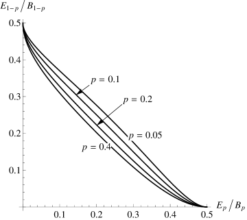
Figure 1: The scaled EER region $\Phi(p)=\{(E_{p}/B_{p},E_{1-p}/B_{1-p}):(E_{p},E_{1-p})\in\mathscr{E}(R_{p},R_{1-p})\}$ for different instances of the compound channel $\mathscr{Q}_{p}\coloneqq\{\mathit{BSC}_{p},\mathit{BSC}_{1-p}\}$.

Proposition 6 implies that for any rate vector $(R_{p},R_{1-p})$ and a particular choice of the estimation threshold $q_{c}$, the above scheme achieves an error exponent $(E_{p},E_{1-p})$ such that

$$E_{p} \geq\frac{D(q_{c}\|p)D(p\|1-p)}{D(q_{c}\|p)+D(p\|1-p)}(1-\gamma_{p}),$$

$$E_{1-p} \geq\frac{D(q_{c}\|1-p)D(p\|1-p)}{D(q_{c}\|1-p)+D(p\|1-p)}(1-\gamma_{1-p})$$

where $\gamma_{p}=R_{p}/C_{p}$ and $\gamma_{1-p}=R_{1-p}/C_{1-p}$.

There are no known upper bounds on the EER. Hence, we compare with the trivial upper bound of the Burnashev exponent of $\mathit{BSC}_{p}$ and $\mathit{BSC}_{1-p}$.

$$\frac{E_{p}}{B_{p}} \geq\frac{D(q_{c}\|p)}{D(q_{c}\|p)+D(p\|1-p)},$$

$$\frac{E_{1-p}}{B_{1-p}} \geq\frac{D(q_{c}\|1-p)}{D(q_{c}\|1-p)+D(p\|1-p)}.$$

Let

$$\varphi(p,q_{c})\coloneqq\left(\frac{E_{p}}{B_{p}},\frac{E_{1-p}}{B_{1-p}}\right)\geq\left(\frac{D(q_{c}\|p)}{D(q_{c}\|p)+D(p\|1-p)},\frac{D(q_{c}\|1-p)}{D(q_{c}\|1-p)+D(p\|1-p)}\right)$$

and

$$\Phi(p) \coloneqq\left\{\left(\frac{E_{p}}{B_{p}},\frac{E_{1-p}}{B_{1-p}}\right):(E_{p},E_{1-p})\in\mathscr{E}(R_{p},R_{1-p})\right\}$$

$$=\{\varphi(p,q_{c}):p<q_{c}<p\}$$

For the scheme proposed in Section 3, $\Phi(p)$ does not depend on the transmission rate $(R_{p},R_{1-p})$. We plot $\Phi(p)$ for different values of $p$ in Figure 1.

6 Conclusion

In the presence of feedback, not knowing the exact channel transition matrix does not result in a loss in capacity. As a result, we can provide an optimistic rate guarantee: any rate less than the capacity of the realized channel is opportunistically achievable, even though we do not know the realized channel before the start of communication. This is in contrast to the pessimistic rate guarantees in compound channel without feedback. More importantly, any rate vector in the optimistic capacity region can be achieved using a simple, training-based coding scheme. The error exponent of this scheme has a negative slope at all rates in the capacity region, even at rates near the boundary of the capacity region.

Our proposed proposed training based scheme is conceptually similar to Yamamoto-Itoh’s scheme. It operates in multiple epochs; each epoch is divided into a message mode and a control mode. A training sequence is transmitted at the beginning of each mode, and the corresponding channel estimate determines the operation during the remainder of the mode.

It may appear that the proposed scheme can be simplified by combining the training phases in each epoch, i.e., have a training phase followed by message and control modes. However, as argued by Tchamkerten and Telatar in [16], such a simplification will lead to error exponents that have zero-slope near capacity. Our results do not contradict the results of [16] because we allow for more sophisticated training. Re-training in the control mode ensures that the error events $\{\hat{W}_{m}(k)\neq W_{m}(k)\}$ and $\{\hat{W}_{c}(k)\neq W_{c}(k)\}$ are independent, which, in turn, is essential to obtain an error exponent of the form $B_{\ell}(1-\gamma_{\ell})$.

One possible way to make the scheme more efficient is to accumulate the training sequences for each phase, i.e., the channel estimation for the message mode and the control mode is based on all past training sequences for that mode. Such an accumulation will improve the finite length performance of the scheme, but does not affect the asymptotic performance because, in the limit, the communication lasts for only one epoch with high probability.

Another possibility to improve the performance of the coding scheme is to use a universal coding scheme for the control mode rather than a training based scheme. This motivates the study of the following communication problem.

Open Problem

Consider the communication of a binary valued message over a compound channel with feedback. Let $\mathscr{Q}=\{Q_{1},\dots,Q_{L}\}$ denote the compound channel, $W\in\{\theta_{0},\theta_{1}\}$ denote the message, $X_{t}$ and $Y_{t}$ denote the channel inputs and output at time $t$, and $\hat{W}$ denotes the decoded message. Consider a variable length coding scheme $(\mathbf{c},\mathbf{g},\tau)$, where $c_{t}$ is the encoding function at time $t$, $g_{t}$ is the decoding function at time $t$, and $\tau$ is a $Y^{t}$-measurable stopping time. The decoded message is

$$\hat{W}=g_{\tau}(Y_{1},\dots,Y_{\tau}).$$

Let $a_{\ell n}$ and $b_{\ell n}$ denote the exponent of the two types of errors, i.e.,

$$a_{\ell n}(\mathbf{c},\mathbf{g},\tau) =\frac{-\log\mathds{P}_{\ell}(\hat{W}=\theta_{1}\mid W=\theta_{0})}{\mathds{E}_{\ell}[\tau\mid W=\theta_{0}]},\quad\ell=1,\dots,L,$$ (47)

$$b_{\ell n}(\mathbf{c},\mathbf{g},\tau) =\frac{-\log\mathds{P}_{\ell}(\hat{W}=\theta_{0}\mid W=\theta_{1})}{\mathds{E}_{\ell}[\tau\mid W=\theta_{1}]},\quad\ell=1,\dots,L.$$ (48)

where $\mathds{P}_{\ell}$ is the induced probability measure when the true channel equals $Q_{\ell}$.

For a sequence $S=\{\mathbf{c}^{(n)},\mathbf{g}^{(n)},\tau^{(n)}\}_{n=1}^{\infty}$ of coding schemes such that

$$\lim_{n\to\infty}\mathds{E}_{\ell}[\tau^{(n)}\mid W=\theta_{i}]=\infty,\quad i=0,1,\quad\ell=1,\dots,L.$$

define the type-I and type-II error exponents of $S$ as

$$a_{\ell*} =\lim_{n\to\infty}a_{\ell n}(\mathbf{c}^{(n)},\mathbf{g}^{(n)},\tau^{(n)}),$$

$$b_{\ell*} =\lim_{n\to\infty}b_{\ell n}(\mathbf{c}^{(n)},\mathbf{g}^{(n)},\tau^{(n)}).$$

Furthermore, define

$$b^{*}_{\ell}=\max_{S:a_{\ell*}(S)=0}b_{\ell*}(S).$$

What is the best type-II exponent $(b^{*}_{1},\dots,b^{*}_{L})$?

Tchamkerten and Telatar [17] studied a similar problem and identified necessary and sufficient conditions under which

$$b^{*}_{\ell}=B_{Q_{\ell}},\quad\ell=1,\dots,L.$$

We are not aware of the solution to the above problem when the conditions of [17] are not satisfied.

Given any sequence $S$ of coding schemes for Problem Open Problem, we can replace the control mode (phases three and four) of the proposed coding scheme by $S$ and achieve an error exponent of

$$(b_{1*}(S)(1-\gamma_{1}),\dots,b_{L*}(S)(1-\gamma_{L})).$$

If $S$ is optimal, the error exponent is

$$(b^{*}_{1}(S)(1-\gamma_{1}),\dots,b^{*}_{L}(S)(1-\gamma_{L})).$$ (49)

We conjecture that no coding scheme can achieve a better error exponent, i.e., (49) is the Pareto frontier of the EER.

When the conditions of [17] are satisfied, we can replace the control mode by the variable length coding scheme proposed in [17], and thereby recover the result of [7]. In fact, in that case, our modified scheme is exactly the same as the variation proposed in [7, Section IV-B]. When the conditions of [17] are not satisfied, the scheme proposed in this paper provide an inner bound on the error exponent region. To find the best error exponents, we need to solve Problem 1.

In this paper, we presented an inner bound on the EER when the compound channel is defined over a finite family. Generalization of the coding scheme to compound channels defined over continuous families is an important and interesting future direction. We believe that solving Problem Open Problem is a critical step in that direction.

References

- [1] J. Wolfowitz, “Simultaneous channels,” Archive for Rational Mechanics and Analysis, pp. 371–386, Nov. 1959.
- [2] D. Blackwell, L. Breiman, and A. J. Thomasian, “The capacity of a class of channels,” The Annals of Mathematical Statistics, vol. 30, no. 4, pp. 1229–1241, Dec. 1959.
- [3] J. Wolfowitz, Coding Theorems of Information Theory. Springer Verlag, 1964.
- [4] B. Shrader and H. Permuter, “Feedback capacity of the compound channel,” IEEE Trans. Inf. Theory, vol. 55, pp. 3629–3644, Aug. 2009.
- [5] A. Lapidoth and P. Narayan, “Reliable communication under channel uncertainty,” IEEE Trans. Inf. Theory, vol. 44, no. 6, pp. 2148–2177, Oct. 1998.
- [6] M. V. Burnashev, “Data transmission over a discrete channel with feedback. Random transmission time,” Problemy peredachi informat︠s︡ii, vol. 12, no. 4, pp. 10–30, 1976.
- [7] A. Tchamkerten and I. E. Telatar, “Variable length coding over an unknown channel,” IEEE Trans. Inf. Theory, vol. 52, no. 5, pp. 2126–2145, May 2006.
- [8] L. Weng, S. S. Pradhan, and A. Anastasopoulos, “Error exponent regions for Gaussian broadcast and multiple-access channels,” IEEE Trans. Inf. Theory, vol. 54, no. 7, pp. 2919–2942, Jul. 2008.
- [9] J. W. Byers, M. Luby, M. Mitzenmacher, and A. Rege, “A digital fountain approach to reliable distribution of bulk data,” SIGCOMM Comput. Commun. Rev., vol. 28, no. 4, pp. 56–67, 1998.
- [10] M. Luby, “LT codes,” in Proceedings of the IEEE Symposium on Foundations of Computer Science, 2002, pp. 271–280.
- [11] A. Shokrollahi, “Raptor codes,” IEEE Trans. Inf. Theory, vol. 6, no. 52, pp. 2551–2567, Jun. 2006.
- [12] H. Yamamoto and K. Itoh, “Asymptotic performance of a modified Schalkwijk-Barron scheme for channels with noiseless feedback,” IEEE Trans. Inf. Theory, vol. 25, no. 6, pp. 729–733, Nov. 1979.
- [13] E. Tuncel, “On error exponents in hypothesis testing,” IEEE Trans. Inf. Theory, vol. 51, no. 8, pp. 2945–2950, Aug. 2005.
- [14] R. E. Blahut, “Hypothesis testing and information theory,” IEEE Trans. Inf. Theory, no. 4, Jul. 1974.
- [15] W. Hoeffding, “Probability inequalities for sums of bounded random variables,” Journal of the American Statistical Association, vol. 58, no. 301, pp. 13–30, Mar. 1963.
- [16] A. Tchamkerten and I. E. Telatar, “On the use of training sequences for channel estimation,” IEEE Trans. Inf. Theory, vol. 52, no. 3, pp. 1171–1176, Mar. 2006.
- [17] ——, “On the universality of Burnashev’s exponent,” IEEE Trans. Inf. Theory, vol. 51, no. 8, pp. 2940–2944, Aug. 2005.