Divergence of logarithm of a unimodular monodromy matrix near the edges of the Brillouin zone

Abstract

A first-order ordinary differential system with a matrix of periodic coefficients $\mathbf{Q}\left(y\right)=\mathbf{Q}\left(y+T\right)$ is studied in the context of time-harmonic elastic waves travelling with frequency $\omega$ in a unidirectionally periodic medium, for which case the monodromy matrix $\mathbf{M}\left(\omega\right)$ implies a propagator of the wave field over a period. The main interest to the matrix logarithm $\ln\mathbf{M}\left(\omega\right)$ is owing to the fact that it yields the ’effective’ matrix $\mathbf{Q}_{\mathrm{eff}}\left(\omega\right)$ of the dynamic-homogenization method. For the typical case of a unimodular matrix $\mathbf{M}\left(\omega\right)$ ($\det\mathbf{M}=1$), it is established that the components of $\ln\mathbf{M}\left(\omega\right)$ diverge as $\left(\omega-\omega_{0}\right)^{-1/2}$ with $\omega\rightarrow\omega_{0},$ where $\omega_{0}$ is the set of frequencies of the passband/stopband crossovers at the edges of the first Brillouin zone. The divergence disappears for a homogeneous medium. Mathematical and physical aspects of this observation are discussed. Explicit analytical examples of $\mathbf{Q}_{\mathrm{eff}}\left(\omega\right)$ and of its diverging asymptotics at $\omega\rightarrow\omega_{0}$ are provided for a simple model of scalar waves in a two-component periodic structure consisting of identical bilayers or layers in spring-mass-spring contact. The case of high contrast due to stiff/soft layers or soft springs is elaborated. Special attention in this case is given to the asymptotics of $\mathbf{Q}_{\mathrm{eff}}\left(\omega\right)$ near the first stopband that occurs at the Brillouin-zone edge at arbitrary low frequency. The link to the quasi-static asymptotics of the same $\mathbf{Q}_{\mathrm{eff}}\left(\omega\right)$ near the point $\omega=0$ is also elucidated.

Keywords: logarithm of a matrix, 1D periodic media, Floquet spectrum, dynamic homogenization, high-contrast structure

1 Introduction

The first-order ordinary differential system

$$\mathbf{Q}\left(y\right)\mathbf{\eta}\left(y\right)=\frac{\mathrm{d}}{\mathrm{d}y}\mathbf{\eta}\left(y\right)$$ (1)

with a $n\times n$ matrix of continuous or piecewise continuous periodic coefficients $\mathbf{Q}\left(y\right)=\mathbf{Q}\left(y+T\right)$ is a classical problem arising in miscellaneous models of applied mathematics and mathematical physics. Its analysis largely relies on the Floquet theorem asserting that the matricant $\mathbf{M}\left(y,0\right)$, which is the fundamental solution of (1) yielding $\mathbf{\eta}\left(y\right)=\mathbf{M}\left(y,0\right)\mathbf{\eta}\left(0\right)$, can be factored into the product

$$\mathbf{M}\left(y,0\right)=\mathbf{L}\left(y\right)\exp\left(i\mathbf{K}y\right),$$ (2)

where $\mathbf{L}\left(y\right)=\mathbf{L}\left(y+T\right)$ ($=\mathbf{M}\left(y_{n},0\right)\exp\left(-i\mathbf{K}y_{n}\right)$ with $y_{n}=y\left(\mathop{\mathrm{m}od}nT\right)$),$\ \mathbf{L}\left(0\right)=\mathbf{I}$ ($\mathbf{I}$ is the identity matrix), and $\mathbf{K}$ is a constant matrix [1]. By (2), $\mathbf{K}$ is defined by the equation

$$\exp\left(i\mathbf{K}T\right)=\mathbf{M}\left(T,0\right)\ \Longrightarrow\ i\mathbf{K}T=\ln\mathbf{M}\left(T,0\right),$$ (3)

where $\mathbf{M}\left(T,0\right)\equiv\mathbf{M}$ is termed the monodromy matrix (its reference to $\left(T,0\right)$ is dropped hereafter). It can be calculated by a number of available methods, e.g., using the Peano series of multiple integrals of $\mathbf{Q}\left(y\right)$, or applying polynomial expansion of $\mathbf{Q}\left(y\right),$ or discretizing $\mathbf{Q}\left(y\right)$. In many problems the system matrix $\mathbf{Q}\left(y\right)$ is a continuous function of a certain control parameter $\omega,$ and hence also $\mathbf{M=M}\left(\omega\right).$ At first glance, the matrix logarithm $\mathbf{K}\left(\omega\right)$ is well-behaved as long as the logarithm of the eigenvalues $q\left(\omega\right)$ of $\mathbf{M}\left(\omega\right)$ is well-behaved. However, it turns out that $\ln\mathbf{M}\left(\omega\right)$ diverges at $\omega\rightarrow\omega_{0},$ where $\omega_{0}$ corresponds to a non-semisimple (not diagonalizable) $\mathbf{M}\left(\omega_{0}\right)$ with a degenerate eigenvalue $q\left(\omega_{0}\right)$ whose values, being taken on the same Riemann sheet of $\ln q,$ are situated on the opposite edges of the cut. This fairly surprising observation seems to have passed unnoticed in the extensive reference literature on the matrix logarithm. The manner in which such a divergence reveals itself in the Floquet formalism is discussed in the present paper in the context where Eq. (1) is associated with time-harmonic elastic waves travelling at frequency $\omega$ in unidirectionally (1D) periodic media. Within this context, the system (1) such that consists of $n=2$ equations and hence is equivalent to Hill’s equation describes scalar acoustic (or electromagnetic) waves [2, 3]; the cases where (1) consists of $n=4,6,8...$ equations corresponds to coupled waves in elastic isotropic or anisotropic media, in piezoelectric or piezomagnetoelectric media, etc. In either of these cases, the monodromy matrix $\mathbf{M}$ is often called the propagator (of the wave field) over the period $T.$

The matrix logarithm $\mathbf{K}\left(\omega\right)$ (3) is a crucial ingredient in the dynamic-homogenization approach. Assuming that $\exp\left(i\mathbf{K}y\right)$ in the 1D Floquet theorem (2) is a relatively slowly varying function, this approach seeks to replace an exact solution $\mathbf{M}\left(y,0\right)$ by its ’slow component’ $\exp\left(i\mathbf{K}y\right)$ and hence to replace the actual periodically inhomogeneous material by an ’homogenized’ medium with spatially constant but frequency dispersive properties described by the ’effective’ matrix

$$\mathbf{Q}_{\mathrm{eff}}\left(\omega\right)=i\mathbf{K}\left(\omega\right),$$ (4)

see e.g. [4, 5, 6]. Obviously, the matrix $\mathbf{Q}_{\mathrm{eff}}$ also provides (regardless of any assumptions) an exact solution $\mathbf{M}\left(nT,0\right)=\exp\left(in\mathbf{K}T\right)$ at the interfaces between the periods. Another aspect of the matrix logarithm $\mathbf{K}\left(\omega\right)$ is related to the Floquet dispersion branches $\omega\left(K\right)$ or $K\left(\omega\right)$. These are determined by the secular equation for $\mathbf{M}$,

$$\det\left[\mathbf{M}\left(\omega\right)-q\left(\omega\right)\mathbf{I}\right]=0,$$ (5)

so that the definition $q=e^{iKT}$ yields $iK\left(\omega\right)T=\ln q\left(\omega\right),$ or else by the formally equivalent secular equation for $\mathbf{K,}$

$$\det\left[\mathbf{K}\left(\omega\right)-K\left(\omega\right)\mathbf{I}\right]=0.$$ (6)

The Floquet spectrum is commonly defined over the first Brillouin zone (BZ) $\mathop{\mathrm{R}e}KT\in\left[-\pi,\pi\right],$ which is related to the zeroth Riemann sheet of the single-valued $\ln q=\ln\left|q\right|+i\arg q$ with the cut $\arg q=\pm\pi$ corresponding to the BZ edges. The frequency intervals where $K$ is real or complex are called passbands and stopbands, respectively.

The paper is concerned with the typical case where $\mathbf{M}\left(\omega\right)$ is unimodular ($\det\mathbf{M}=1$) and so the BZ edges contain the passband/stopband crossovers at a set of frequencies $\omega=\omega_{0}$ associated with a degenerate pair of eigenvalues $q\left(\omega_{0}\right)$ of$\ \mathbf{M}\left(\omega_{0}\right).$ According to the background outlined in §2, this is the case for a normal propagation across an arbitrary anisotropic periodic structure or for an arbitrary propagation direction in the presence of appropriately oriented symmetry plane. The original material of this work consists of two parts, § 3 and §4. The first part (§3) deals with the problem in general. It is shown that the matrix $\ln\mathbf{M}\left(\omega\right)=i\mathbf{K}\left(\omega\right)T,$ and hence $\mathbf{Q}_{\mathrm{eff}},$ must have components diverging as $\left(\omega-\omega_{0}\right)^{-1/2}$ when $\omega\rightarrow\omega_{0},$ i.e. when the real Floquet branches tend to the BZ edges or the complex part of $\pm K=\pi/T+i\mathop{\mathrm{I}m}K$ tends to zero. The eigenspectrum of $\mathbf{K}\left(\omega\right)$ certainly remains well-behaved for any $\omega$ infinitesimally close to $\omega_{0}$; however, computing the Floquet spectrum $K\left(\omega\right)$ specifically from Eq. (6) may become numerically unstable at $\omega$ close to $\omega_{0}.$ A transition is explained from a weakly inhomogeneous to perfectly homogeneous elastic medium, for which $\ln\mathbf{M}\left(\omega\right)$ certainly does not diverge. The second part (§4) presents detailed analytical examples of $\mathbf{Q}_{\mathrm{eff}}\left(\omega\right)$ and of its diverging asymptotics for $\omega\rightarrow\omega_{0}$ for the shear-horizontal wave in a periodic structure composed of piecewise homogeneous bilayers or layers in spring-mass-spring contact. Particular attention is given to the high-contrast case with either a soft layer in the bilayer or with a soft spring in the interfacial joint. The interest to this case lies in the fact that the first stopband at the BZ edges and hence the local divergence of $\mathbf{Q}_{\mathrm{eff}}\left(\omega\right)$ occurs at low frequency that may in principle be made arbitrarily small. To this end, a link to the regular asymptotics of the same $\mathbf{Q}_{\mathrm{eff}}\left(\omega\right)$ near the point $\omega=0$ is also elucidated. The basic points of the study are summarized in §5. Some technical aspects of the derivations of §3 and §4 are detailed in the Appendix.

2 Background

Consider elastic waves in a 1D-periodic infinite anisotropic non-absorbing medium without sources. Choose the periodicity direction as the axis $Y$ and denote the (least) period by $T,$ so that the density and the elasticity tensor satisfy $\rho\left(y\right)=\rho\left(y+T\right)$ and $\mathbf{c}\left(y\right)=\mathbf{c}\left(y+T\right)$, respectively. Take the axis $X$ in the sagittal plane spanned by $Y$ and by the direction to the observation point. Applying Fourier transforms in time and in $X$ brings in the frequency $\omega$ and wavenumber $k_{x}$ as the (real) parameters of the problem.

The equation of motion and the linear stress-strain law may be combined into the system (1) of, generally, six equations. The periodic matrix of coefficients $\mathbf{Q}\left(y\right)$ defined through $\rho\left(y\right),$ $\mathbf{c}\left(y\right)$ and $\omega$, $k_{x},$ is pure imaginary and has the Hamiltonian structure

$$\mathbf{Q}\left(y\right)=\mathbf{TQ}^{\mathrm{T}}\left(y\right)\mathbf{T,}$$ (7)

where the superscript ^T means transpose and $\mathbf{T}$ is the matrix with zero diagonal and identity off-diagonal 3$\times$3 blocks (see e.g. [7] for the details).

In the following we deal with the essentially typical case of a medium with at least a single symmetry plane $m$ orthogonal to the axis $X$ or $Y.$ Then the trace of $\mathbf{Q}\left(y\right)$ is zero for any $y$. Therefore, by the Jacobi identity, $\mathbf{M}\left(y,0\right)$ is unimodular and hence so is the monodromy matrix $\mathbf{M}\equiv\mathbf{M}\left(T,0\right),$ i.e.

$$\det\mathbf{M}=1.$$ (8)

The identities (7) and (8) together ensure that for every eigenvalue $q_{\alpha}$ of $\mathbf{M}$, there is a corresponding eigenvalue $q_{\beta}=1/q_{\alpha}$ where $\alpha,\beta=1,...,6.$ This property has been established in [9] for a piecewise constant $\mathbf{Q}\left(y\right)$ and $m\perp Y;$ its generalization for any piecewise continuous $\mathbf{Q}\left(y\right)$ and for $m\perp X$ is obvious. Note that no stipulation of any material symmetry is needed if the wave propagates strictly along the periodicity direction $Y$ (i.e. if $k_{x}=0$), which is when (8) is always true. Also note that the out-of-plane motion with respect to the symmetry plane $m\perp Z$ of a monoclinic body (which has no other symmetry planes) can be cast in the form with property (8), see [8].

Let $\omega$ be a single free dispersion parameter ($k_{x}$ is fixed or expressed through $\omega$). Each pair $q_{\beta}\left(\omega\right)=1/q_{\alpha}\left(\omega\right)$ corresponds to a set of dispersion curves $K_{\alpha}\left(\omega\right)=-K_{\beta}\left(\omega\right)$ in the BZ $\mathop{\mathrm{R}e}K_{\alpha,\beta}T\in\left[-\pi,\pi\right],$ which are symmetric about the line $K=0.$ In view of (8), the eigenvalues $q=1$ and $q=-1,$ occurring, respectively, at the centre and edges of the BZ, are assuredly degenerate. We are interested in the case $q=-1,$ which is associated with a sequence of passband/stopband crossover points at the BZ edges, and specifically in the behaviour of the matrix $\ln\mathbf{M}=i\mathbf{K}T$ in the vicinity of these points.

3 Divergence of $\mathbf{K}\left(\omega\right)$ near the BZ edges

3.1 Derivation

Denote by $\omega=\omega_{0}$ the frequency, at which some pair of eigenvalue branches $q_{1}\left(\omega\right)=1/q_{2}\left(\omega\right)$ of the monodromy matrix $\mathbf{M}\left(\omega\right)$ fall into two-fold degeneracy $q_{1}\left(\omega_{0}\right)=q_{2}\left(\omega_{0}\right)=-1$ rendering $\mathbf{M}\left(\omega_{0}\right)$ non-semisimple. Consider a function $\ln q=\ln\left|q\right|+i\arg q$ defined on the zeroth Riemann sheet with a cut $\arg q=\pm\pi$ passing through $-1.$ Let $\omega$ lying in the stopband or passband tend to $\omega_{0}$ from, respectively, above or below. Then $q_{1}\left(\omega\right)$ and $q_{2}\left(\omega\right)$ tend to $e^{\pm i\pi},$ thus approaching their degenerate value $-1$ from the opposite sides of the cut for $\ln q$, and, correspondingly, $\ln q_{1,2}\left(\omega\right)=iK_{1,2}\left(\omega\right)T$ tend to $\pm i\pi,$ meaning that two Floquet branches tend to the opposite edges of the BZ.

This is indeed nothing else than a very standard setup. The state of affairs is, however, not so trivial when the same limit $\omega\rightarrow\omega_{0}$ is applied to the matrix logarithm $\ln\mathbf{M}\left(\omega\right)=i\mathbf{K}\left(\omega\right)T.$ It is natural to specify it by asking that both eigenvalues $\ln q_{1,2}\left(\omega\right)$ of $\ln\mathbf{M}\left(\omega\right)$ satisfy the above-mentioned definition of $\ln q$ (the issue of alternative definitions of $\ln\mathbf{M}$ is addressed in §3.1 and in §A.2 of Appendix). As we have just observed, these eigenvalues tend to $\pm i\pi$ as $\omega\rightarrow\omega_{0},$ i.e. they do not approach each other in contrast to the eigenvalues $q_{1}\left(\omega\right)\rightarrow q_{2}\left(\omega\right)$ of $\mathbf{M}\left(\omega\right)$. This signals a singularity of $\ln\mathbf{M}\left(\omega\right)$ on the path $\omega\rightarrow\omega_{0}.$

Let us analyze the local behaviour of $\ln\mathbf{M}\left(\omega\right)$ for $\omega=\omega_{0}+\Delta\omega$ ($\left|\Delta\omega/\omega_{0}\right|\ll 1$). With reference to (8), denote

$$q_{1,2}\left(\omega_{0}+\Delta\omega\right)\approx q_{d}\pm\delta q\underset{\omega\rightarrow\omega_{0}}{\rightarrow}q_{1,2}\left(\omega_{0}\right)\equiv q_{d}=-1,$$ (9)

where $\delta q$ means the leading-order correction in the small parameter $\Delta\omega/\omega_{0}$. For brevity, assume the case of 2$\times$2 matrices (the same derivation for the general $n\times n$ case is detailed in Appendix, § A1). A polynomial formula for a function of a 2$\times$2 matrix $\mathbf{M}$ with eigenvalues $q_{1}\neq q_{2}$ has a simple form

$$f\left(\mathbf{M}\right)=\frac{q_{2}f\left(q_{1}\right)-q_{1}f\left(q_{2}\right)}{q_{2}-q_{1}}\mathbf{I}+\frac{f\left(q_{2}\right)-f\left(q_{1}\right)}{q_{2}-q_{1}}\mathbf{M,\ }$$ (10)

see e.g. [10]. Taking (10) for $\mathbf{M}\left(\omega_{0}+\Delta\omega\right)=\mathbf{M}\left(\omega_{0}\right)+\mathbf{\Delta M}$ with $q_{1,2}\left(\omega\right)$ given by (9) yields

$$f\left[\mathbf{M}\left(\omega_{0}+\Delta\omega\right)\right]=\frac{f_{01}+f_{02}}{2}\mathbf{I}+\left[\frac{f_{01}-f_{02}}{2\delta q}+f^{\prime}\left(q_{d}\right)\right]\left[\mathbf{M}\left(\omega_{0}\right)+\mathbf{\Delta M}-q_{d}\mathbf{I}\right]+\mathbf{O}\left(\delta q\right),$$ (11)

where $f_{01,02}=\lim_{\omega\rightarrow\omega_{0}}f\left(q_{1,2}\left(\omega\right)\right)$ and $\mathbf{O}$ is a matrix symbol ’of the order of’. For the case in hand $f=\ln$ and $f_{01,02}=\ln\left(e^{\pm i\pi}\right),$ whence (11) becomes

$$\ln\mathbf{M}\left(\omega_{0}+\Delta\omega\right)=\left(\frac{i\pi}{\delta q}+\frac{1}{q_{d}}\right)\left[\mathbf{M}\left(\omega_{0}\right)-q_{d}\mathbf{I}\right]+\frac{i\pi}{\delta q}\mathbf{\Delta M}+\mathbf{O}\left(\delta q,\mathbf{\Delta M}\right).$$ (12)

Since $\mathbf{M}\left(\omega_{0}\right)-q_{d}\mathbf{I}$ is non-zero for a non-semisimple $\mathbf{M}\left(\omega_{0}\right)$ while $\delta q$ tends to zero with $\Delta\omega\rightarrow 0,$ we conclude from Eq. (12) that the matrix logarithm $\ln\mathbf{M}\left(\omega\right),$ and thus $\mathbf{K}\left(\omega\right),$ must have components tending to infinity when $\omega\rightarrow\omega_{0}.$ Note in passing that an identically zero determinant of the first matrix term on the right-hand side of (12) does certainly not preclude but, on the contrary, underlies (with due regard for the next term) the necessary identity $\det\left[\ln\mathbf{M}\left(\omega\right)\right]\rightarrow\pi^{2}$ as $\omega\rightarrow\omega_{0}.$

Let us now find an asymptotic rate of divergence of $\ln\mathbf{M}\left(\omega\right)$ in terms of $\Delta\omega\left(\equiv\omega-\omega_{0}\right).$ For a non-semisimple $\mathbf{M}$ of 2$\times$2 dimension, the leading-order dependence $\delta q\sim\left(\omega-\omega_{0}\right)^{1/2}$ obviously follows from a quadratic secular equation (5). For the general $n\times n$ case, the same trend is easy to infer from the leading-order Taylor expansion of $D\left(q,\omega\right)\equiv\det\left[\mathbf{M}\left(\omega\right)-q\mathbf{I}\right]$ about the point of double degeneracy $q_{1,2}\left(\omega_{0}\right)=q_{d},$ which leads to

$$\left(\delta q\right)^{2}=B\Delta\omega,\ B=-2\left(\frac{\partial D/\partial\omega}{\partial^{2}D/\partial q^{2}}\right)_{\omega_{0},q_{d}}.$$ (13)

Omitting details (see e.g. [11]), it suffices to note that $B$ is generally non-zero for non-semisimple $\mathbf{M}\left(\omega_{0}\right).$ Thus, by (12), $\ln\mathbf{M}\left(\omega\right),$ and hence $\mathbf{K}\left(\omega\right),$ diverges as $\left(\omega-\omega_{0}\right)^{-1/2}$ with $\omega\rightarrow\omega_{0}.$ An explicit form of the coefficient $B$ will be exemplified in §4.

3.2 Discussion

A few formal remarks are in order. First it is reiterated that even though the components of the dealt-with matrix $\ln\mathbf{M}\left(\omega\right)=i\mathbf{K}\left(\omega\right)T$ diverge as $\omega\rightarrow\omega_{0},$ its eigenvalues $\ln q_{1,2}=iK_{1,2}\left(\omega\right)T$ remain formally well-defined so long as $\omega\neq\omega_{0}.$ It is also understood that the exponential of this $\ln\mathbf{M}\left(\omega\right)$ at any $\omega\neq\omega_{0}$ certainly reproduces (continuous) $\mathbf{M}\left(\omega\right)$. Regarding the infinity of $\ln\mathbf{M}\left(\omega\right)$ precisely at $\omega=\omega_{0},$ which is when $\delta q=0$ on the right-hand side of (12), it simply tells us that the conventional definition of $\ln\mathbf{M}\left(\omega\right),$ which refers both eigenvalues $\ln q_{1,2}\left(\omega\right)$ to the zeroth Riemann sheet of $\ln q$ with the cut $\arg q=\pm\pi$ fixing the edges of the BZ $\mathop{\mathrm{R}e}KT\in\left[-\pi,\pi\right],$ precludes this matrix function of $\omega$ from reaching the limiting point $\omega_{0}$ of the path $\omega\rightarrow\omega_{0}$ continuously.

It is clear from the above that shifting the cut in the $q$-plane away from the point $q=-1$ while keeping $\ln q_{1,2}$ on the same Riemann sheet leads to a different matrix logarithm $\ln\mathbf{M}\left(\omega\right)$ that has degenerate eigenvalues $\ln q_{1}\left(\omega_{0}\right)=\ln q_{2}\left(\omega_{0}\right)$ and hence is well-behaved at $\omega=\omega_{0}$ and around it. However, this ’gain’ for $\omega$ near $\omega_{0}$ is at the expense of one or another essential deficiency elsewhere for the redefined $\ln\mathbf{M}\left(\omega\right).$ For instance, if the eigenvalues $\ln q_{1,2}$ of $\ln\mathbf{M}\left(\omega\right)$ are taken on the zeroth Riemann sheet with the cut $\arg q=0,2\pi,$ then this $\ln\mathbf{M}\left(\omega\right)$ has the same divergence $\sim\left(\omega-\omega_{01}\right)^{-1/2}$ due to the degeneracy $q_{1,2}\left(\omega_{01}\right)=1$ at the set $\omega_{01}$ of passband/stopband crossovers occurring at $K=0,2\pi.$ An exception is the origin point $\omega=0,$ where $\mathbf{M=I}$ and so any $\ln\mathbf{M}$ is continuous; however, the low-frequency onset of $\ln\mathbf{M}$ defined by taking the cut $\arg q=0,2\pi$ has no physical sense (see Appendix, §A2). Another possibility is to use a cut $\arg q=\varphi,\varphi-2\pi$ at $\varphi\neq\pi n,$ e.g., at $\varphi$ such that $0<\varphi<\pi.$ Then $\ln\mathbf{M,}$ whose eigenvalues $\ln q_{1,2}=\pm iKT$ lie on the zeroth Riemann sheet, is well-behaved with $\left|\arg q\right|=\left|KT\right|$ growing from zero but only until reaching $\varphi,$ where there is a jump to a different matrix $\ln\mathbf{M,}$ for which the eigenvalue $\ln q_{1}$ has to be shifted from $\arg q_{1}=KT$ to $\mathrm{\arg}q_{1}=KT-2\pi$ with $KT>0$ increasing above $\varphi$. Note that a similar piecewise discontinuity pertains in the BZ $\mathop{\mathrm{R}e}KT\in\left[-\pi,\pi\right]$ to the logarithm of $\mathbf{M}$ that is not unimodular ($\det\mathbf{M}\neq 1$). Thus, using any ’unconventional’ definition of the logarithm of $\mathbf{M}$ based on shifting the cut from the point $q=-1$ is hardly an alternative.

It remains to settle a natural question concerning the case of a homogeneous elastic material, for which the matrix $\mathbf{Q}$ is constant, hence $\mathbf{M}=\exp\left(\mathbf{Q}T\right),$ and so $\ln\mathbf{M}$ merely returns the ’initial’ $\mathbf{Q}T,$ which is certainly continuous in $\omega.$ ’Technically’, the difference with the case of a periodic medium is that a constant $\mathbf{Q}$ keeps $\mathbf{M}\left(\omega_{0}\right)$ diagonalizable (semisimple) at the degeneracy point $q_{1}\left(\omega_{0}\right)=q_{2}\left(\omega_{0}\right)=-1$ under discussion. Assuming $\mathbf{M}\left(\omega_{0}\right)=q_{d}\mathbf{I}$ in Eq. (12), its first term turns to zero and thus a continuous $\ln\mathbf{M}\left(\omega_{0}+\Delta\omega\right)$ is defined by the second term of (12), in which $\mathbf{\Delta M}\sim\left(\omega-\omega_{0}\right)$ and $\delta q\sim\left(\omega-\omega_{0}\right)$ (the latter being due to $B=0$ in (13) for a semisimple $\mathbf{M}\left(\omega_{0}\right)$ [11]). A transition to (or from) a homogeneous material from (or to) a weakly (periodically) inhomogeneous one is also evident: given a small parameter $\epsilon$ of elastic inhomogeneity, $\mathbf{M}\left(\omega_{0}\right)-q_{d}\mathbf{I}$ is scaled by $\epsilon$ and $\delta q$ is scaled by $\left(\epsilon\Delta\omega\right)^{1/2},$ hence, by (12), the singularity of $\ln\mathbf{M}\left(\omega\right)$ at $\omega\rightarrow\omega_{0}$ is proportional to $\left(\epsilon/\Delta\omega\right)^{1/2}$ and disappears at $\epsilon=0.$

In conclusion, let us outline some exceptional cases that are theoretically possible due to ’incidental’ occurrence of $\mathbf{M}\left(\omega_{0}\right)$ in a peculiar form. First, a non-semisimple $\mathbf{M}\left(\omega_{0}\right)$ does not preclude vanishing of the leading-order coefficient $B$ (13)₂ [11]; if it happens to be zero then $\left(\delta q\right)^{2}$ is given by the higher-order terms of the Taylor series of $D\left(q,\omega\right)$ about $\omega_{0}$, in which case Eq. (12) (where $\mathbf{M}\left(\omega_{0}\right)\neq q_{d}\mathbf{I}$) leads to $\ln\mathbf{M}\left(\omega\right)\sim\left(\omega-\omega_{0}\right)^{-m/2}$ with an integer $m\geq 2.$ Secondly, a (periodically) inhomogeneous medium $\mathbf{M}\left(\omega_{0}\right)$ does not rule out a possibility for $\mathbf{M}\left(\omega_{0}\right)$ at a degeneracy point to remain semisimple (such an option is usually associated with a stopband of zero width). Finally, a semisimple $\mathbf{M}\left(\omega_{0}\right)$ may, in principle, also cause diverging $\ln\mathbf{M}\left(\omega_{0}+\Delta\omega\right)$ - it is the case when $\delta q\sim\left(\omega-\omega_{0}\right)^{1+\left(m/2\right)}$ with $m>0$ due to incidentally vanishing higher-order derivatives $\partial^{2}D/\partial\omega^{2},\partial^{2}D/\partial q\partial\omega$ etc. in the Taylor series of $D\left(q,\omega\right)$ about $\omega_{0}$, whence $\ln\mathbf{M}\left(\omega\right)$ for $\omega\rightarrow\omega_{0}$ diverges owing to the term $\left(\delta q\right)^{-1}\mathbf{\Delta M}\sim$ $\left(\omega-\omega_{0}\right)^{-m/2}$ in Eq. (12).

4 Examples of $\mathbf{Q}_{\mathrm{eff}}=i\mathbf{K}$

4.1 Bilayered unit cell

This section is intended to illuminate the preceding general development by way of its application to simple examples of a scalar acoustic wave in a periodically repeated sequence of pairs of homogeneous layers. With this purpose, we first remind the 2$\times$2 setup for an arbitrary 1D-periodic medium [2, 3] and detail the formulas describing the ’effective’ matrix $\mathbf{Q}_{\mathrm{eff}}=i\mathbf{K}$ for this framework. Then we further elaborate $\mathbf{Q}_{\mathrm{eff}}$ for the case of a bilayered unit cell.

4.1.1 2$\times$2 setup

Consider a 2$\times$2 unimodular monodromy matrix $\mathbf{M}\left(\omega\right)\mathbf{.}$ Its eigenvalues

$$q_{1,2}=\frac{1}{2}\mathrm{trace\,}\mathbf{M}\pm R,\ \mathrm{where\ }R\equiv\frac{1}{2}\sqrt{\left(\mathrm{trace\,}\mathbf{M}\right)^{2}-4}\left(=\frac{q_{1}-q_{2}}{2}\right),$$ (14)

define the Floquet wavenumbers

$$iK_{1,2}T=\pm iKT=\ln q_{1,2}=\pm i\arccos\left(\frac{1}{2}\mathrm{trace\,}\mathbf{M}\right)=\pm 2i\arccos\left(\frac{1}{2}\sqrt{\mathrm{trace\,}\mathbf{M}+2}\right);$$ (15)

and the equation

$$\mathrm{trace\,}\mathbf{M=}-2$$ (16)

defines the set of frequencies $\omega=\omega_{0}$ of passband/stopband crossovers at the BZ edges $KT=\pm\pi$ where $q_{1}\left(\omega_{0}\right)=q_{2}\left(\omega_{0}\right)\equiv q_{d}=-1,$ see [2, 3].

Introduce the 2$\times$2 ’effective’ matrix $\mathbf{Q}_{\mathrm{eff}}=i\mathbf{K,}$ which is related to $\mathbf{M}$ by the equality $\mathbf{M}=\exp\left(i\mathbf{K}T\right)$ and which has eigenvalues (15) understood under the standard definition of the functions $\ln$ and $\arccos,$ so that $\mathop{\mathrm{R}e}KT\in\left[-\pi,\pi\right].$ Then Eq. (10) specified for $f\left(\mathbf{M}\right)\equiv\ln\mathbf{M}$ gives

$$\mathbf{Q}_{\mathrm{eff}}\left(\omega\right)=\frac{iK}{R}\left[\mathbf{M-}\frac{1}{2}\left(\mathrm{trace\,}\mathbf{M}\right)\mathbf{I}\right].$$ (17)

The same result may certainly be obtained by equating $\mathbf{M}$ to $\exp\left(i\mathbf{K}T\right),$ which follows from the same (10) (re-adjusted to $f\left(\mathbf{K}\right)$) in the form

$$\exp\left(i\mathbf{K}T\right)=\left(\cos KT\right)\mathbf{I}+\left(i\frac{\sin KT}{K}\right)\mathbf{K=}\frac{1}{2}\left(\mathrm{trace\,}\mathbf{M}\right)\mathbf{I}+\frac{R}{K}\mathbf{K}$$ (18)

due to using the condition $K_{1,2}=\pm K$ equivalent to fixing the appropriate definition of matrix logarithm $\ln\mathbf{M}.$

Consider now a vicinity of the BZ edge. Eqs. (14), (15) expand in small $\Delta\omega=\omega-\omega_{0}$ as

$$\begin{array}[]{c}q_{1,2}\left(\omega\right)\mid_{\omega\approx\omega_{0}}=-1\pm\sqrt{B\Delta\omega}+O\left(\Delta\omega\right),\ K\left(\omega\right)T\mid_{\omega\approx\omega_{0}}=\pi+i\sqrt{B\Delta\omega}+O\left(\Delta\omega\right),\\ R\left(\omega\right)\mid_{\omega\approx\omega_{0}}=\sqrt{B\Delta\omega+O\left[\left(\Delta\omega\right)^{2}\right]},\end{array}$$ (19)

where it is denoted

$$B=-\left(\frac{\mathrm{d}}{\mathrm{d}\omega}\mathrm{trace\,}\mathbf{M}\right)_{\omega_{0}},$$ (20)

which is non-zero for a non-semisimple $\mathbf{M}\left(\omega_{0}\right)$ (barring the theoretical exceptions mentioned in the end of §3.2). Inserting (19) and (20) in (17) yields

$$\mathbf{Q}_{\mathrm{eff}}\left(\omega\right)_{\omega\approx\omega_{0}}=\frac{i\pi-\sqrt{B\Delta\omega}+O\left(\Delta\omega\right)}{\sqrt{B\Delta\omega+O\left[\left(\Delta\omega\right)^{2}\right]}}\left\{\mathbf{A}+\left[\left(\frac{\mathrm{d}\mathbf{M}}{\mathrm{d}\omega}\right)_{\omega_{0}}+\frac{1}{2}B\mathbf{I}\right]\Delta\omega+\mathbf{O}\left(\Delta\omega\right)^{2}\right\},$$ (21)

where $\mathbf{A}$ denotes a non-zero nilpotent matrix

$$\mathbf{A=M}\left(\omega_{0}\right)-q_{d}\mathbf{I=M}\left(\omega_{0}\right)+\mathbf{I\ \ (A}^{2}=\mathbf{0).\ }$$ (22)

Eq. (21) elaborates (12) (with due regard for $\mathbf{\Delta M/}\delta q\sim\mathbf{O}\left(\delta q\right)$). Note also that Eq. (19)₃ for $R,$ defined in (14)${}_{2},$ to leading order reads $\delta q=\sqrt{B\Delta\omega}$ which is recognized as the equation (13)₁. Correspondingly, the definition (20) of the coefficient $B$ is equivalent to Eq. (13)${}_{2},$ which specializes for the given case (of 2$\times$2 $\mathbf{M}$ with $q_{d}=-1$ at $\omega_{0}$) as

$$B=-\left[\frac{\mathrm{d}}{\mathrm{d}\omega}\det\left(\mathbf{M}-q\mathbf{I}\right)\right]_{\omega_{0}}=\mathrm{trace}\left[\mathbf{A}\left(\frac{\mathrm{d}\mathbf{M}}{\mathrm{d}\omega}\right)_{\omega_{0}}\right].$$ (23)

Expansion (21) shows that the ’effective’ matrix $\mathbf{Q}_{\mathrm{eff}}\left(\omega\right)$ has well-behaved eigenvalues $\pm iK\left(\omega\right)\rightarrow\pm i\pi/T$ at $\omega\rightarrow\omega_{0},$ while its components diverge due to non-zero $\mathbf{A}$ with a common factor $\sim\left(\omega-\omega_{0}\right)^{-1/2}$. It is also seen from Eqs. (21)-(23) that $\mathbf{A}$ and $B$ for a weakly inhomogeneous unit cell can in general be scaled by the same small parameter $\epsilon$ ($=0$ for a homogeneous limit), and so the singularity of $\mathbf{Q}_{\mathrm{eff}}\left(\omega\right)$ at $\omega\rightarrow\omega_{0}$ is scaled by $\left(\epsilon/\Delta\omega\right)^{1/2}$ as argued in §3.

4.1.2 $\mathbf{Q}_{\mathrm{eff}}\$for a bilayered unit cell

Let us narrow our analysis to the case of a two-component piecewise constant unit cell. Specifically, we consider the shear horizontal (SH) wave in a periodic structure of perfectly bonded pairs of isotropic homogeneous infinite layers $j=1,2$, each with constant density $\rho_{j},$ shear modulus $\mu_{j}$ and thickness $d_{j}.$ For the sake of the brevity of explicit formulas, assume the wave $u\left(y\right)$ propagating along the axis $Y$ normal to the interfaces ($k_{x}=0$). Hooke’s law $\sigma\left(y\right)=\mu_{j}u^{\prime}\left(y\right)$ and the equation of motion $\sigma^{\prime}\left(y\right)=-\rho_{j}\omega^{2}u\left(y\right)$ combine into the system (1) with the state vector $\mathbf{\eta}\left(y\right)=\left(i\omega u,\ \sigma\right)^{\mathrm{T}}$ and the piecewise-constant periodic 2$\times$2 system matrix

$$\mathbf{Q}_{j}=i\omega s_{j}\left(\begin{array}[]{cc}0&Z_{j}^{-1}\\ Z_{j}&0\end{array}\right),\ j=1,2,$$ (24)

which leads to the propagator $\mathbf{M}\left(T,0\right)=\mathrm{e}^{\mathbf{Q}_{2}d_{2}}\mathrm{e}^{\mathbf{Q}_{1}d_{1}}\equiv\mathbf{M}\left(\omega\right)$ through the period $T=d_{1}+d_{2}$ (the monodromy matrix) in the form

$$\mathbf{M}\left(\omega\right)=\left(\begin{array}[]{cc}\cos\psi_{2}\cos\psi_{1}-\frac{Z_{1}}{Z_{2}}\sin\psi_{2}\sin\psi_{1}&\frac{i}{Z_{1}}\cos\psi_{2}\sin\psi_{1}+\frac{i}{Z_{2}}\sin\psi_{2}\cos\psi_{1}\\ iZ_{1}\cos\psi_{2}\sin\psi_{1}+iZ_{2}\sin\psi_{2}\cos\psi_{1}&\cos\psi_{2}\cos\psi_{1}-\frac{Z_{2}}{Z_{1}}\sin\psi_{2}\sin\psi_{1}\end{array}\right),$$ (25)

where $s_{j}=\sqrt{\rho_{j}/\mu_{j}}$ is the slowness, $Z_{j}=\sqrt{\rho_{j}\mu_{j}}$ the impedance and $\psi_{j}=\omega s_{j}d_{j}$ the phase shift over a layer. Passing in (25) to an oblique propagation amounts to merely premultiplying $\psi_{j}$ and $Z_{j}$ by $\sqrt{1-s_{x}^{2}/s_{j}^{2}}$ with a fixed $s_{x}=k_{x}/\omega$. Inserting $\mathbf{M}$ into the basic relations (14)-(16) provides the textbook equations implicitly defining the Floquet spectrum $\omega\left(K\right)$ and its stopband bounds $\omega=\omega_{0}$ at the BG edge for a bilayered unit cell, e.g.[2].

The 2$\times$2 ’effective’ matrix $\mathbf{Q}_{\mathrm{eff}}=i\mathbf{K}$ for a bilayered unit cell follows from (17) and (25) in the form

$$\mathbf{Q}_{\mathrm{eff}}\left(\omega\right)=\frac{iK}{R}\begin{pmatrix}-\frac{1}{2}\left(\frac{Z_{1}}{Z_{2}}-\frac{Z_{2}}{Z_{1}}\right)\sin\psi_{2}\sin\psi_{1}&\frac{i}{Z_{1}}\cos\psi_{2}\sin\psi_{1}+\frac{i}{Z_{2}}\sin\psi_{2}\cos\psi_{1}\\ {i}{Z_{1}}\cos\psi_{2}\sin\psi_{1}+{i}{Z_{2}}\sin\psi_{2}\cos\psi_{1}&\frac{1}{2}\left(\frac{Z_{1}}{Z_{2}}-\frac{Z_{2}}{Z_{1}}\right)\sin\psi_{2}\sin\psi_{1}\end{pmatrix}.$$ (26)

It is easy to check that the eigenvalues of this matrix are $\pm iK$, and that it reduces to (24)₁ when $Z_{1}=Z_{2},$ $s_{1}=s_{2}.$ As another consistency test, we note that (26) provides the well-known low-frequency asymptotics of $\mathbf{Q}_{\mathrm{eff}},$ whose diagonal and off-diagonal components expand in, respectively, even and odd powers of $i\omega$ as follows:

$$\begin{array}[]{c}\mathbf{Q}_{\mathrm{eff}}\left(\omega\right)_{\omega/\omega_{0}\ll 1}=\left\langle\mathbf{Q}\right\rangle+\frac{d_{1}d_{2}}{2T}\left(\mathbf{Q}_{2}\mathbf{Q}_{1}-\mathbf{Q}_{1}\mathbf{Q}_{2}\right)+...\\ =i\omega\left(\begin{array}[]{cc}0&\left\langle\mu^{-1}\right\rangle\\ \left\langle\rho\right\rangle&0\end{array}\right)+\frac{1}{2}\left(i\omega\right)^{2}\kappa T\left(\begin{array}[]{cc}1&0\\ 0&-1\end{array}\right)+...,\end{array}$$ (27)

where

$$\begin{array}[]{c}\mathrm{\ }\left\langle\mathbf{Q}\left(\omega\right)\right\rangle=\mathbf{Q}_{1}\frac{d_{1}}{T}+\mathbf{Q}_{2}\frac{d_{2}}{T},\ \left\langle\mu^{-1}\right\rangle=\frac{1}{\mu_{1}}\frac{d_{1}}{T}+\frac{1}{\mu_{2}}\frac{d_{2}}{T},\\ \ \left\langle\rho\right\rangle=\rho_{1}\frac{d_{1}}{T}+\rho_{2}\frac{d_{2}}{T},\ \kappa=\frac{d_{1}d_{2}}{T^{2}}\left(\frac{\rho_{1}}{\mu_{2}}-\frac{\rho_{2}}{\mu_{1}}\right).\end{array}$$ (28)

Additional explicit insight is gained by noticing that $\mathrm{trace\,}\mathbf{M}+2$ with $\mathbf{M}$ given by (25) can be factored as

$$\begin{array}[]{c}\mathrm{trace\,}\mathbf{M}+2=f_{+}f_{-},\\ f_{\pm}=\frac{1}{\sqrt{Z_{1}Z_{2}}}\left[\left(Z_{1}+Z_{2}\right)\cos\frac{\psi_{1}+\psi_{2}}{2}\pm\left(Z_{1}-Z_{2}\right)\cos\frac{\psi_{1}-\psi_{2}}{2}\right],\end{array}$$ (29)

whence Eqs. (14), (15) provide

$$iK\left(\omega\right)T=\ln\left(\frac{f_{+}f_{-}}{2}-1+R\right)=2i\arccos\frac{\sqrt{f_{+}f_{-}}}{2},\ R=\sqrt{f_{+}f_{-}\left(\frac{f_{+}f_{-}}{4}-1\right)},$$ (30)

and Eq. (16) takes the form

$$f_{+}f_{-}=0,$$ (31)

showing that the set $\omega=\omega_{0}$ consists of two families given by zeros of $f_{\pm}.$ Evidently, this split reveals the symmetric/antisymmetric decoupling of the problem. As a result, the expansion (21) of $\mathbf{Q}_{\mathrm{eff}}\left(\omega\right)$ about the points $\omega=\omega_{0},$ when applied to the matrix $\mathbf{Q}_{\mathrm{eff}}$ (26) in hand, admits compact formulas for its leading-order parameters $B$ (20) and $\mathbf{A}$ (22) as follows:

$$\begin{array}[]{c}B=-\left(f_{\mp}\frac{\mathrm{d}f_{\pm}}{\mathrm{d}\omega}\right)_{\omega_{0}}=\mp\frac{1}{\omega_{0}}\left(\frac{Z_{1}}{Z_{2}}-\frac{Z_{2}}{Z_{1}}\right)\left(\psi_{1}\sin\psi_{2}+\psi_{2}\sin\psi_{1}\right),\\ \mathbf{A=\pm}\left(\begin{array}[]{cc}\cos\psi_{1}+\cos\psi_{2}&\frac{i}{Z_{1}}\sin\psi_{1}-\frac{i}{Z_{2}}\sin\psi_{2}\\ iZ_{2}\sin\psi_{2}-iZ_{1}\sin\psi_{1}&-\cos\psi_{1}-\cos\psi_{2}\end{array}\right),\end{array}$$ (32)

where $\psi_{j}=\omega_{0}s_{j}d_{j}$ are referred to $\omega_{0},$ and the upper or lower sign corresponds to $f_{+}=0$ or $f_{-}=0$ in (31), respectively (see §A3 of Appendix for derivation of (32)₂). The derivative $\left(\mathrm{d}\mathbf{M/}\mathrm{d}\omega\right)_{\omega_{0}},$ which also appears in (21), can be obtained due to $\mathbf{M}=\mathrm{e}^{\mathbf{Q}_{2}d_{2}}\mathrm{e}^{\mathbf{Q}_{1}d_{1}}$ in the form expressed through the matrices $\mathbf{Q}_{j}$ (24) and $\mathbf{A}$ as

$$\left(\frac{\mathrm{d}\mathbf{M}}{\mathrm{d}\omega}\right)_{\omega_{0}}=\frac{1}{\omega_{0}}\left(d_{2}\mathbf{Q}_{2}\mathbf{M}+d_{1}\mathbf{MQ}_{1}\right)_{\omega_{0}}=\frac{T}{\omega_{0}}\left[\frac{d_{2}}{T}\mathbf{Q}_{2}\left(\omega_{0}\right)\mathbf{A}+\frac{d_{1}}{T}\mathbf{AQ}_{1}\left(\omega_{0}\right)-\left\langle\mathbf{Q}\left(\omega_{0}\right)\right\rangle\right].$$ (33)

Its plugging in (23)₂ and taking note of $\mathbf{A}^{2}=\mathbf{0}$ yields another definition of the coefficient $B$,

$$B=-\frac{T}{\omega_{0}}\mathrm{trace}\left[\mathbf{A}\left\langle\mathbf{Q}\left(\omega_{0}\right)\right\rangle\right]\mathrm{\,},$$ (34)

which for the given case of a bilayered unit cell is equivalent to (20) and (23). It is easy to verify that (34) with (28) and (32)₂ leads to (32)${}_{1}.$

The following analysis for highly contrasting layers and for layers in spring-mass-spring contact makes an extensive use of the factorization (29) and the consequent formulas.

4.1.3 High-contrast case

It is instructive to specialize the above considerations to the case of high contrast between the material properties of two layers composing the unit cell. Suppose that, e.g., the second layer is much softer than the first one:

$$\mu_{2}/\mu_{1}\equiv\varepsilon^{2}\ \left(=>s_{2}\sim\varepsilon^{-1},\ Z_{2}\sim\varepsilon\right),\ \mathrm{where\ }0<\varepsilon\ll 1.$$ (35)

The main interest of the high-contrast case is that the first stopband at the BZ edge occurs in the low-frequency range, which is scaled by $\varepsilon$ and implies $\psi_{1}=O\left(\varepsilon\right),\ \psi_{2}=O\left(1\right).$ In this range, the propagator (25) is approximated to leading order in $\varepsilon$ as

$$\mathbf{M}\left(\omega\right)_{\psi_{1}=O\left(\varepsilon\right)}=\left(\begin{array}[]{cc}\cos\psi_{2}-\beta\sin\psi_{2}&\frac{i}{Z_{2}}\sin\psi_{2}\\ iZ_{2}\left(\sin\psi_{2}+\beta\cos\psi_{2}\right)&\cos\psi_{2}\end{array}\right)\ ,$$ (36)

where

$$\beta\left(\omega\right)\equiv\frac{Z_{1}\psi_{1}}{Z_{2}}\left(=\omega\frac{\rho_{1}d_{1}}{\sqrt{\rho_{2}\mu_{2}}}=\frac{\rho_{1}d_{1}}{\rho_{2}d_{2}}\psi_{2}\right);$$ (37)

and Eq. (16) with $\mathbf{M}$ (36) defines the stopband bounds $\omega=\omega_{0}$ by

$$\cos\psi_{2}-\frac{\beta}{2}\sin\psi_{2}=-1\ \Leftrightarrow\cos\frac{\psi_{2}}{2}\left(\cos\frac{\psi_{2}}{2}-\frac{\beta}{2}\sin\frac{\psi_{2}}{2}\right)=0.\$$ (38)

The latter, factorized, form is Eq. (31) with approximate $f_{\pm}$ (29)${}_{2}.$ So the first stopband is bounded by the least roots of $f_{+}=0$ and $f_{-}=0$ which, to leading order in $\varepsilon,$ are the first zeros of the cofactors of (38)${}_{2}.$ The upper bound corresponding to $f_{+}=0$ is close to the first thickness resonance $\psi_{2}\left(=\omega s_{2}d_{2}\right)=\pi$ of the soft layer. Denote the lower bound corresponding to $f_{-}=0$ by $\Omega~{}\left(=\min\omega_{0}\right).$ It is approximated by the least root of equation

$$\tan\left(\psi_{2}/2\right)=2/\beta,$$ (39)

which involves coupling of the layers. Note in passing resemblance and dissimilarity between this simple model (see also §4.2) and the textbook case of a high-contrast diatomic lattice [2].

With a view to highlight the low-frequency behaviour of $\mathbf{Q}_{\mathrm{eff}}\left(\omega\right)$, let us focus our attention on $\omega$ ranging from $\omega\approx\Omega$ and going down the first Floquet branch to $\omega=0.$ Substituting (36) in (26) yields

$$\mathbf{Q}_{\mathrm{eff}}\left(\omega\right)=\frac{iK}{R}\left(\begin{array}[]{cc}-\frac{\beta}{2}\sin\psi_{2}&\frac{i}{Z_{2}}\sin\psi_{2}\\ iZ_{2}\left(\sin\psi_{2}+\beta\cos\psi_{2}\right)&\frac{\beta}{2}\sin\psi_{2}\end{array}\right),$$ (40)

where by (30) and (38)

$$\begin{array}[]{c}iK\left(\omega\right)T=\ln\left(\cos\psi_{2}-\frac{\beta}{2}\sin\psi_{2}+R\right)=2i\arccos\left[\cos\frac{\psi_{2}}{2}\left(\cos\frac{\psi_{2}}{2}-\frac{\beta}{2}\sin\frac{\psi_{2}}{2}\right)\right]^{1/2},\\ R\left(\omega\right)=\left[2\sin\psi_{2}\left(\frac{\beta}{2}\cos\frac{\psi_{2}}{2}+\sin\frac{\psi_{2}}{2}\right)\left(\frac{\beta}{2}\sin\frac{\psi_{2}}{2}-\cos\frac{\psi_{2}}{2}\right)\right]^{1/2}.\end{array}$$ (41)

The singular term for $\mathbf{Q}_{\mathrm{eff}}\left(\omega\right)$ (40) as $\omega$ tends to the first stopband bound $\Omega$ is $\mathbf{Q}_{\mathrm{eff}}\left(\omega\right)\varpropto\frac{i\pi}{\sqrt{B\Delta\omega}}\mathbf{A}$ (see (21)) with $\sqrt{\Delta\omega}=i\sqrt{\Omega-\omega}$ and

$$B=\frac{1}{\Omega}\left[\beta\left(\psi_{2}+\sin\psi_{2}\right)\right]_{\omega=\Omega},\ \mathbf{A}=\frac{2}{1+\left(2/\beta\right)^{2}}\left(\begin{array}[]{cc}-1&\frac{2i}{Z_{2}\beta}\\ iZ_{2}\beta/2&1\end{array}\right)_{\omega=\Omega}\mathbf{.}$$ (42)

Eq. (42) follows from (32) which is taken with the lower sign (since $\Omega$ is defined by $f_{-}=0$) and confined to leading order in $\varepsilon$ (in accordance with the accuracy of (36) and hence of (40)). The asymptotics of the same $\mathbf{Q}_{\mathrm{eff}}\left(\omega\right)$ (40) near the origin point $\omega=0$ is given by Eq. (27) with

$$\left\langle\mu^{-1}\right\rangle=\frac{1}{\mu_{2}}\frac{d_{2}}{T},\ \kappa=\frac{d_{1}d_{2}}{T^{2}}\frac{\rho_{1}}{\mu_{2}},$$ (43)

which also implies taking leading order in the high-contrast parameter $\varepsilon.$ Note that $B$ provided in (42)₁ satisfies Eq. (34) with $\left\langle\mathbf{Q}\right\rangle$ given by (43).

4.2 Layers in spring-mass-spring contact

As another example, consider propagation of the SH wave through a structure of identical layers of thickness $T$ in spring-mass-spring contact. Denote the rigidity of each of two springs by $\gamma$ and the mass by $m.$ Note that the physical dimension of $m$ is voluminal density times length. The monodromy matrix $\mathbf{M\equiv M}\left(T,0\right)$ for the state vector $\mathbf{\eta}=\left(i\omega u,\ \sigma\right)^{\mathrm{T}}$ is $\mathbf{M}=\mathbf{M}_{\mathrm{int}}\mathbf{M}_{l},$ where $\mathbf{M}_{l}=\exp\left(\mathbf{Q}T\right)$ is the propagator across the layer with $\mathbf{Q}$ given by (24) (no subscripts $j=1,2$), and $\mathbf{M}_{\mathrm{int}}$ is the propagator across the spring-mass-spring interface:

$$\mathbf{M}_{\mathrm{int}}=\left(\begin{array}[]{cc}1-\frac{\omega^{2}m}{\gamma}&\frac{2i\omega}{\gamma}\left(1-\frac{\omega^{2}m}{2\gamma}\right)\\ i\omega m&1-\frac{\omega^{2}m}{\gamma}\end{array}\right)=\left(\begin{array}[]{cc}1-\frac{2\omega^{2}}{\Omega_{r}^{2}}&\frac{2i\omega}{\gamma}\left(1-\frac{\omega^{2}}{\Omega_{r}^{2}}\right)\\ \frac{2i\omega\gamma}{\Omega_{r}^{2}}&1-\frac{2\omega^{2}}{\Omega_{r}^{2}}\end{array}\right),$$ (44)

where $\Omega_{r}=\sqrt{2\gamma/m}$ is the resonant frequency of this joint. Thus

$$\mathbf{M}\left(\omega\right)=\left(\begin{array}[]{cc}\left(1-\frac{2\omega^{2}}{\Omega_{r}^{2}}\right)\cos\psi-\frac{2\omega Z}{\gamma}\left(1-\frac{\omega^{2}}{\Omega_{r}^{2}}\right)\sin\psi&\frac{i}{Z}\left(1-\frac{2\omega^{2}}{\Omega_{r}^{2}}\right)\sin\psi+\frac{2i\omega}{\gamma}\left(1-\frac{\omega^{2}}{\Omega_{r}^{2}}\right)\cos\psi\\ iZ\left(1-\frac{2\omega^{2}}{\Omega_{r}^{2}}\right)\sin\psi+\frac{2i\omega\gamma}{\Omega_{r}^{2}}\cos\psi&\left(1-\frac{2\omega^{2}}{\Omega_{r}^{2}}\right)\cos\psi-\frac{2\omega\gamma}{Z\Omega_{r}^{2}}\sin\psi\end{array}\right).$$ (45)

A factorized form (31) of the equation (16) defining the stopbands at the edge of the BZ holds with

$$\begin{array}[]{c}f_{+}=4\left[\left(1-\psi^{2}\frac{m}{\rho T}\frac{\mu}{2\gamma T}\right)\cos\frac{\psi}{2}-\frac{m}{2\rho T}\psi\sin\frac{\psi}{2}\right],\\ f_{-}=\cos\frac{\psi}{2}-\frac{\mu}{\gamma T}\psi\sin\frac{\psi}{2},\end{array}$$ (46)

where $\omega^{2}/\Omega_{r}^{2}=\psi^{2}m\mu/2\rho\gamma T^{2}$ is used to write $f_{\pm}$ as functions of the phase shift $\psi=\omega T\sqrt{\rho/\mu}.$ It is seen that $f_{+}\left(\psi\right)$ depends on both spring and mass parameters $\gamma T/\mu$ and $m/\rho T,$ while $f_{-}\left(\psi\right)$ depends on $\mu/\gamma T$ only.

Let us again specialize our consideration to the high-contrast case of a similar ’stiff/soft’ nature, now by assuming a relatively small rigidity

$$\gamma T/\mu\ll 1$$ (47)

of the springs supporting the mass. Like before, we are interested in the first stopband at the BZ edge. Given (47), the least roots $\psi_{\pm}$ of $f_{\pm}=0$ and the corresponding stopband bounds $\Omega_{\pm}$ to leading order are

$$\begin{array}[]{c}\psi_{+}=\min\left(\sqrt{\frac{2\gamma T}{\mu}\frac{\rho T}{m}},~{}\pi\right)\ \Rightarrow\ \Omega_{+}=\min\left(\Omega_{r},\ \Omega_{l}\right)=\min\left(\sqrt{\frac{2\gamma}{m}},\ \frac{\pi}{T}\sqrt{\frac{\mu}{\rho}}\right);\\ \psi_{-}=\sqrt{\frac{2\gamma T}{\mu}}\ \Rightarrow\ \Omega_{-}=\sqrt{\frac{2\gamma}{\rho T}},\end{array}\$$ (48)

where $\Omega_{l}$ is the frequency of the thickness resonance of the layer. The question is which of $\Omega_{+}$ and $\Omega_{-}$ is the lower frequency bound. Since $\Omega_{-}^{2}/\Omega_{r}^{2}=m/\rho T,$ it is evident that a heavy mass $m\gg\rho T$ ensures $\Omega_{+}=\Omega_{r}<\Omega_{-};$ a ’medium heavy’ mass $m\sim\rho T$ implies commensurate $\Omega_{+}=\Omega_{r}\sim\Omega_{-},$ and a light mass $m\ll\rho T$ ensures $\Omega_{-}<\Omega_{+}.$ For the two former cases, the whole first stopband is confined to the low-frequency range in the sense that both its bounds provide a small phase $\psi\ll 1.$ In the latter case of a light mass, decreasing the small parameter $m/\rho T$ keeps the lower bound at $\psi_{-}\ll 1$ and lifts the upper bound up until the phase $\psi_{+}$ reaches $\pi,$ i.e. $\Omega_{r}$ reaches $\Omega_{l}$.

Consider the range $\psi\ll 1$ containing one or both bounds ($\Omega_{-}$ or $\Omega_{-}$ and $\Omega_{+}=\Omega_{r}$, respectively) of the first stopband at the BZ edge. Expanding (45) to leading order in small $\psi,$ bearing in mind (47), and using the notations (48) of $\Omega_{-}$ and $\Omega_{r}$ yields

$$\mathbf{M}\left(\omega\right)=\left(\begin{array}[]{cc}1-\frac{2\omega^{2}}{\Omega_{r}^{2}}-4\frac{\omega^{2}}{\Omega_{-}^{2}}\left(1-\frac{\omega^{2}}{\Omega_{r}^{2}}\right)&\frac{2i\omega}{\gamma}\left(1-\frac{\omega^{2}}{\Omega_{r}^{2}}\right)\\ \frac{2i\omega\gamma}{\Omega_{-}^{2}}\left(1-\frac{2\omega^{2}}{\Omega_{r}^{2}}+\frac{\Omega_{-}^{2}}{\Omega_{r}^{2}}\right)&1-\frac{2\omega^{2}}{\Omega_{r}^{2}}\end{array}\right),$$ (49)

which observes $\det\mathbf{M}=1$. Inserting (49) in (17) gives

$$\mathbf{Q}_{\mathrm{eff}}\left(\omega\right)=\frac{iK}{R}\left(\begin{array}[]{cc}-2\frac{\omega^{2}}{\Omega_{-}^{2}}\left(1-\frac{\omega^{2}}{\Omega_{r}^{2}}\right)&\frac{2i\omega}{\gamma}\left(1-\frac{\omega^{2}}{\Omega_{r}^{2}}\right)\\ \frac{2i\omega\gamma}{\Omega_{-}^{2}}\left(1-\frac{2\omega^{2}}{\Omega_{r}^{2}}+\frac{\Omega_{-}^{2}}{\Omega_{r}^{2}}\right)&2\frac{\omega^{2}}{\Omega_{-}^{2}}\left(1-\frac{\omega^{2}}{\Omega_{r}^{2}}\right)\end{array}\right),$$ (50)

in which

$$\begin{array}[]{c}iK\left(\omega\right)T=\ln\left(2\alpha-1+R\right)=2i\arccos\sqrt{\alpha},\ R\left(\omega\right)=2i\sqrt{\alpha\left(1-\alpha\right)}\\ \mathrm{with}\ \alpha=\left(1-\omega^{2}/\Omega_{r}^{2}\right)\left(1-\omega^{2}/\Omega_{-}^{2}\right).\end{array}$$ (51)

The latter follows from a similar expansion of $f_{\pm}\left(\psi\right)$ (46) at $\psi\ll 1\$and $\gamma T/\mu\ll 1,$ approximating the l.h.s. of Eq. (31) as $f_{+}f_{-}=4\alpha$ and plugging it into (30).

According to (50) and (51), the matrix $\mathbf{Q}_{\mathrm{eff}}\left(\omega\right),$ as expected, experiences the square-root singularity at the BZ edge; however, it does so in a different way when $\omega$ approaches either $\Omega_{-}$ (light mass) or $\Omega_{r}$ (if $\Omega_{r}$ fulfils $\psi\ll 1;$ heavy mass). By (49) and (50), all components of the matrix $\mathbf{A=M}\left(\Omega_{-}\right)-\mathbf{I}$ are non-zero and hence all components of $\mathbf{Q}_{\mathrm{eff}}\left(\omega\right)$ diverge when $\omega\rightarrow\Omega_{-}.$ This is a typical option for a singularity of $\mathbf{Q}_{\mathrm{eff}}\left(\omega\right).$ On the other hand, $\mathbf{A=M}\left(\Omega_{r}\right)-\mathbf{I}$ has only left off-diagonal component being non-zero, and hence only this component of $\mathbf{Q}_{\mathrm{eff}}\left(\omega\right)$ diverges when $\omega\rightarrow\Omega_{r}$ while the others tend to zero. This is rather an unusual option, which is due to the approximations underlying a simple form (49) and (50) of $\mathbf{M}$ and $\mathbf{Q}_{\mathrm{eff}}.$ The transition between the two above options occurs at $\Omega_{-}=\Omega_{r}$ (i.e. $m=\rho T$), in which case $\omega_{0}=\Omega_{-}=\Omega_{r}$ implies the stopband of zero width that yields a semisimple $\mathbf{M}\left(\omega_{0}\right)=-\mathbf{I}$ so that $\mathbf{Q}_{\mathrm{eff}}\left(\omega\right)$ is well-behaved at $\omega\rightarrow\omega_{0}$ (it is one of the extraordinary possibilities mentioned in the end of §3.2). For either of these cases, the low-frequency asymptotics of $\mathbf{Q}_{\mathrm{eff}}\left(\omega\right)$ (50) is given by (27) with the effective properties taken to leading order in the soft-spring parameter (47), i.e., with

$$\left\langle\mu^{-1}\right\rangle=\frac{2}{\gamma T},\ \ \left\langle\rho\right\rangle=\rho+\frac{m}{T},\ \kappa=\frac{2\rho}{\gamma T},$$ (52)

where $\gamma_{s}=\gamma/2$ is the rigidity of two identical springs in series (cf. (43)).

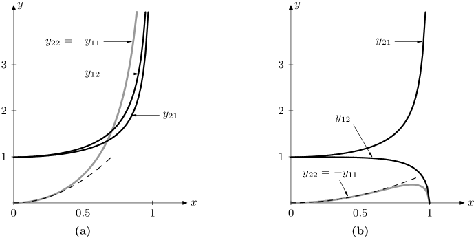
Figure 1: Frequency dependence of components of the ’effective’ matrix $\mathbf{Q}_{\mathrm{eff}}$ (50) in the first passband, which is (a) $\omega\in\left[0,\Omega_{-}\right]$ with $\Omega_{-}^{2}/\Omega_{r}^{2}=1/3$ and (b) $\omega\in\left[0,\Omega_{r}\right]$ with $\Omega_{-}^{2}/\Omega_{r}^{2}=3.$ Black curves are the off-diagonal components $ij=12,~{}21$ normalized by their statically averaged values; grey curves are diagonal components, whose leading low-frequency evaluation ($\sim\omega^{2}$) is shown by dashed line. The curves definition is specified in the text.

The two types of singular behaviour of the ’effective’ matrix $\mathbf{Q}_{\mathrm{eff}}\left(\omega\right)$ defined by (50), (51) are illustrated in Fig. 1. It displays the off-diagonal components normalized by their statically-averaged values $\left\langle\mathbf{Q}\right\rangle_{ij}$ ($\sim\omega$, see (27) with (52)_1,2) and compares the diagonal components to their leading low-frequency term ($\sim\omega^{2},$ see (27) with (52)₃). Specifically, the plotted curves are defined as $y_{ij}\left(x\right)=\frac{1}{\left\langle\mathbf{Q}\right\rangle_{ij}}\left(\mathbf{Q}_{\mathrm{eff}}\right)_{ij}$ ($ij=12,21$) and $y_{ii}\left(x\right)=T\left(\mathbf{Q}_{\mathrm{eff}}\right)_{ii}$ ($y_{22}=-y_{11}$) with $x=\omega/\Omega_{-}$ when $\Omega_{-}^{2}=\left(1/3\right)\Omega_{r}^{2}$ (Fig. 1a) and with $x=\omega/\Omega_{r}$ when $\Omega_{-}^{2}=3\Omega_{r}^{2}$ (Fig. 1b), where $\Omega_{-}^{2}/\Omega_{r}^{2}=m/\rho T$ $\left(\gg\gamma T/2\mu\right).$

Note in conclusion that passing to the case of an oblique propagation ($k_{x}=\omega s_{x}\neq 0,$ see note to (25)) implies replacing the entries of layer density $\rho$ by $\rho-s_{x}^{2}\mu$. Moreover, this case enables further ’ramification’ of the spring-mass-spring model by means of recasting the point mass $m$ as an ’elastic’ mass $m\left(1-c_{T}^{2}s_{x}^{2}\right)$ with its own shear velocity $c_{T}$ (then $\Omega_{r}^{2}$ becomes $\Omega_{r}^{2}=2\gamma/m\left(1-c_{T}^{2}s_{x}^{2}\right)$). It is also noted that the case of layers in ’pure spring’ contact (i.e. without a mass) is described by the above formulas taken with $m=0$ ($\Omega_{r}^{2}\rightarrow\infty$) and with $\gamma_{s}=\gamma/2$ as the rigidity of the spring joint, or else by the formulas of §4.1 taken in the limit $d_{2}\rightarrow 0$, $\mu_{2}\rightarrow 0$ while keeping $\gamma_{s}=\mu_{2}/d_{2}$ finite.

5 Summary

Components of the matrix logarithm $\ln\mathbf{M},$ where $\mathbf{M=M}\left(T,0\right)$ is a unimodular propagator matrix relating the acoustic wave field with a frequency $\omega$ at one and the other ends of a period $T$ of 1D-periodic anisotropic medium, have been shown to diverge when the frequency $\omega$ tends to the values $\omega_{0}$ of passband/stopband crossovers occurring at the edge of the first Brillouin zone (BZ). Explicit analytical examples of the ’effective’ matrix $\mathbf{Q}_{\mathrm{eff}}\left(\omega\right)\left(\equiv i\mathbf{K}\left(\omega\right)\right)=\frac{1}{T}\ln\mathbf{M}\left(\omega\right)$ and of its diverging asymptotics near the BZ edges were provided for the simple case of a scalar waves in a two-component periodic structure of several types, including its high-contrast model when the least of $\omega_{0}$ may be made arbitrarily small.

Whereas the components of matrix $\mathbf{Q}_{\mathrm{eff}}$ diverge at $\omega\rightarrow\omega_{0}$, it is understood that $\mathbf{Q}_{\mathrm{eff}}$ for any $\omega\neq\omega_{0}$ yields a continuous $\mathbf{M}=\exp\left(\mathbf{Q}_{\mathrm{eff}}T\right)$ and has a continuous eigenspectrum which is in one-to-one correspondence with that of $\mathbf{M.}$ Thus, invoking a diverging $\mathbf{Q}_{\mathrm{eff}}$ for formulating a time-harmonic wave propagation through a finite or infinite number of periods cannot create any difficulty, because this phenomenon can be fully described via $\mathbf{M}$ and its eigenspectrum. At the same time, divergence of components of $\mathbf{Q}_{\mathrm{eff}}$ calls for careful interpretation if the governing system (1) is taken with $\mathbf{Q}_{\mathrm{eff}}$ in place of the actual matrix of coefficients $\mathbf{Q}\left(y\right)$ and is then viewed in the same sense as the ’true’ system (1), i.e., as incorporating the equation of motion and the constitutive law, but now with the constant coefficients $\mathbf{Q}_{\mathrm{eff}}\left(\omega\right)$ of the fictitious homogenized medium.

Explicit results of this paper can readily be adjusted to other physical problems whose mathematical formulation admits reduction to Eq. (1), see e.g. [12]. Further development is underway to analyze the Floquet dispersion near an arbitrary passband/stopband crossover occurring anywhere in the BZ of 1D-periodic structure. Another interest lies in the potential extension of the analytical means of the paper to more complicated cases, like in [13], whose exact mathematical statement does not reduce to (1).

Acknowledgement. AAK and ANN wish to express thanks to the Laboratoire de Mécanique Physique (LMP) of the Université Bordeaux 1 for the hospitality. The visit of AAK to the LMP has been supported by the grant ANR-08-BLAN-0101-01 from the Agence Nationale de la Recherche. The authors are grateful to O. Poncelet for numerous stimulating discussions.

APPENDIX

A1. On the divergence of the logarithm of a $n\times n$ matrix $\mathbf{M}(\omega)\vskip 3.0pt plus 1.0pt minus 1.0pt$

Let $\mathbf{M}(\omega)$ be a $n\times n$ non-singular ($\det\mathbf{M}\neq 0$) matrix, continuous in $\omega,$ with eigenvalues $q_{j}(\omega).$ Denote $\mathbf{M}(\omega_{0})=\mathbf{M}_{0},$ $q_{j}(\omega_{0})=q_{j}^{0}$ and suppose that $q_{1}^{0}=q_{2}^{0}\equiv q_{d}$ while all other $q_{j}^{0}$ ($j\neq 1,2$) are distinct. Consider a small neighbourhood of $\omega_{0},$ where

$$\mathbf{M}(\omega)=\mathbf{M}_{0}+\mathbf{o}(1),\ q_{j}(\omega)=q_{j}^{0}+o(1),$$ (53)

and all $q_{j}(\omega)$ ($j=1,2,...,n$) are distinct. Assume that the matrix $\mathbf{M}_{0}$ with a degenerate eigenvalue $q_{d}$ is non-semisimple, i.e., that the Jordan form $\mathbf{J}_{0}$ of $\mathbf{M}_{0}$ is

$$\mathbf{J}_{0}=\mathbf{P}\oplus\mathbf{S\ }\mathrm{with}\mathbf{\ P}=q_{d}\mathbf{I}_{2}+\mathbf{R,\ R}=\left(\begin{array}[]{cc}0&1\\ 0&0\end{array}\right),\ \mathbf{S}=\mathrm{diag}\left(q_{3}^{0},...,q_{n}^{0}\right),$$ (54)

where $\mathbf{I}_{m}$ denotes the $m\times m$ identity matrix. Thus the spectral decomposition of $\mathbf{M}(\omega)$ is

$$\begin{array}[]{c}\mathbf{M}(\omega)=\mathbf{C}\left(\omega\right)\mathrm{diag}\left(q_{1}\left(\omega\right),...,q_{n}\left(\omega\right)\right)\mathbf{C}^{-1}\left(\omega\right)\ \mathrm{for\ }\omega\neq\omega_{0},\\ \mathbf{M}_{0}=\mathbf{C}_{0}\mathbf{J}_{0}\mathbf{C}_{0}^{-1}\ \mathrm{for\ }\omega=\omega_{0},\end{array}$$ (55)

where $\mathbf{C}\left(\omega\right)$ and $\mathbf{C}_{0}$ are matrices whose columns are linear independent eigenvectors of, respectively, $\mathbf{M}(\omega)$ and $\mathbf{M}_{0}$ (note that $\mathbf{C}_{0},$ which includes a generalized eigenvector of $\mathbf{M}_{0},$ is certainly not $\mathbf{C}\left(\omega_{0}\right),$ which is singular).

Introduce a logarithm of $\mathbf{M}\left(\omega\right)$ with $\omega\neq\omega_{0},$

$$\begin{array}[]{c}\ln\mathbf{M}\left(\omega\right)=\mathbf{C}\left(\omega\right)\mathrm{diag}\left(\ln q_{1}\left(\omega\right),...,\ln q_{n}\left(\omega\right)\right)\mathbf{C}^{-1}\left(\omega\right),\\ \mathrm{where}\ \ln q_{j}=\ln|q_{j}|+i(\arg q_{j}+2\pi k_{j}),\ k_{j}\in\mathbb{Z}.\end{array}$$ (56)

This is a general definition in the sense that, while observing indeed the equality $\exp\left[\ln\mathbf{M}\left(\omega\right)\right]=\mathbf{M}\left(\omega\right),$ it permits taking each $\ln q_{j}$ in (56₂) on any $k_{j}$-th Riemann sheet. Let us further suppose that

$$\ln q_{1}^{0}-\ln q_{2}^{0}=2\pi i,$$ (57)

which implies either that $q_{1}\left(\omega\right)$ and $q_{2}\left(\omega\right)$ tending to $q_{d}$ as $\omega\rightarrow\omega_{0}$ are defined on adjacent Riemann sheets ($k_{1}-k_{2}=1$) and $q_{d}$ is away from the cut, or, alternatively, that $q_{1}\left(\omega\right)$ and $q_{2}\left(\omega\right)$ are taken on the same Riemann sheet ($k_{1}=k_{2}$ in (56₂)) with the cut such that $q_{1}^{0}$ and $q_{2}^{0}$ are located on its opposite edges. The latter option with $k_{1,2}=0$ is directly related to the physical context discussed in this paper.

Our purpose is to show that, under the aforementioned assumptions, the asymptotics of $\ln\mathbf{M}\left(\omega\right)$ at $\omega\rightarrow\omega_{0}$ is

$$\begin{array}[]{c}\ln\mathbf{M}\left(\omega\right)=\frac{2\pi i}{q_{1}\left(\omega\right)-q_{2}\left(\omega\right)}\mathbf{A}+\mathbf{o}\left(\frac{1}{q_{1}\left(\omega\right)-q_{2}\left(\omega\right)}\right)\ \mathrm{with\ }\\ \mathbf{A}=\mathbf{C}_{0}\left[\mathbf{J}_{0}-\mathrm{diag}\left(q_{d},q_{d},q_{3}^{0},...,q_{n}^{0}\right)\right]\mathbf{C}_{0}^{-1}=\mathbf{C}_{0}(\mathbf{R}\oplus\mathbf{0}_{n-2})\mathbf{C}_{0}^{-1}\neq\mathbf{0}_{n},\end{array}$$ (58)

where $\mathbf{0}_{m}$ is $m\times m$ zero matrix and the other entries have been defined above.

The derivation of (58) is based on the Lagrange-Sylvester formula [10] with due regard for (53), (55₂) and (57). Along these lines, we manipulate $\ln\mathbf{M}\left(\omega\right)$ as follows (omitting for brevity the argument $\omega$ of $\mathbf{M}\left(\omega\right)$ and $q_{j}\left(\omega\right)$):

$$\begin{array}[]{c}\ln\mathbf{M}=\sum_{k=1}^{n}\left(\prod_{j\neq k}\frac{\mathbf{M}-q_{j}\mathbf{I}_{n}}{q_{k}-q_{j}}\right)\ln q_{k}\\ =\sum_{k=1}^{n}\left(\prod_{j\neq k}\frac{\mathbf{M}_{0}-q_{j}^{0}\mathbf{I}_{n}}{q_{k}-q_{j}}\right)\ln q_{k}^{0}+\mathbf{o}\left(\frac{1}{q_{1}-q_{2}}\right)\\ =\sum_{k=1}^{2}\left(\prod_{j\neq k}\frac{\mathbf{M}_{0}-q_{j}^{0}\mathbf{I}_{n}}{q_{k}-q_{j}}\right)\ln q_{k}^{0}+\mathbf{o}\left(\frac{1}{q_{1}-q_{2}}\right)\\ =\left(\prod_{j\geq 3}\frac{\mathbf{M}_{0}-q_{j}^{0}\mathbf{I}_{n}}{q_{d}-q_{j}^{0}}\right)\frac{\mathbf{M}_{0}-q_{d}\mathbf{I}_{n}}{q_{1}-q_{2}}(\ln q_{1}^{0}-\ln q_{2}^{0})+\mathbf{o}\left(\frac{1}{q_{1}-q_{2}}\right)\\ =\frac{2\pi i}{q_{1}-q_{2}}\left(\prod_{j\geq 3}\frac{\mathbf{M}_{0}-q_{j}^{0}\mathbf{I}_{n}}{q_{d}-q_{j}^{0}}\right)(\mathbf{M}_{0}-q_{d}\mathbf{I}_{n})+\mathbf{o}\left(\frac{1}{q_{1}-q_{2}}\right)\\ =\frac{2\pi i}{q_{1}-q_{2}}\mathbf{C}_{0}\left[\left(\prod_{j\geq 3}\frac{\mathbf{J}_{0}-q_{j}^{0}\mathbf{I}_{n}}{q_{d}-q_{j}^{0}}\right)(\mathbf{J}_{0}-q_{d}\mathbf{I}_{n})\right]\mathbf{C}_{0}^{-1}+\mathbf{o}\left(\frac{1}{q_{1}-q_{2}}\right).\end{array}$$ (59)

Next we invoke (54) and observe that

$$\left(\prod_{j\geq 3}\frac{\mathbf{J}_{0}-q_{j}^{0}\mathbf{I}_{n}}{q_{d}-q_{j}^{0}}\right)(\mathbf{J}_{0}-q_{d}\mathbf{I}_{n})=\mathbf{R}\oplus\mathbf{0}_{n-2},$$ (60)

which is due to

$$\begin{array}[]{c}\left(\prod_{j\geq 3}\frac{\mathbf{P}-q_{j}^{0}\mathbf{I}_{2}}{q_{d}-q_{j}^{0}}\right)(\mathbf{P}-q_{d}\mathbf{I}_{2})=\left[\prod_{j\geq 3}\left(\mathbf{I}_{2}+\frac{1}{q_{d}-q_{j}^{0}}\mathbf{R}\right)\right]\mathbf{R}\\ =\left(\mathbf{I}_{2}+\sum_{j=3}^{n}\frac{1}{q_{d}-q_{j}^{0}}\mathbf{R}\right)\mathbf{R}=\mathbf{R;}\\ \left(\prod_{j\geq 3}\frac{\mathbf{S}-q_{j}^{0}\mathbf{I}_{n-2}}{q_{d}-q_{j}^{0}}\right)(\mathbf{S}-q_{d}\mathbf{I}_{n-2})=\mathbf{0}_{n-2}.\end{array}$$ (61)

Note that an essential simplification of (60) is a consequence of $\mathbf{R}^{2}=\mathbf{0}_{2},$ yielding (61₁). Finally, inserting (60) into (59) delivers the sought result (58). Admitting $\mathbf{A}=\mathbf{0}_{n}$ in (58) would lead to a contradiction $\mathbf{0}_{n}=\mathbf{C}_{0}^{-1}\mathbf{A}\mathbf{C}_{0}=\mathbf{R}_{0}\oplus\mathbf{0}_{n-2}\neq\mathbf{0}_{n}$, hence $\mathbf{A}\neq\mathbf{0}_{n}.\ \blacksquare$

Equation (58) shows that the condition (57) leads to divergence of $\ln\mathbf{M}\left(\omega\right)$ with $q_{1}\left(\omega\right)\rightarrow q_{2}\left(\omega\right)$ at $\omega\rightarrow\omega_{0}.$ For a unimodular $\mathbf{M,}$ taking (58) with $q_{1}\left(\omega\right)-q_{2}\left(\omega\right)\approx 2\delta q$ gives $\ln\mathbf{M}\left(\omega\right)=\frac{\pi i}{\delta q}\mathbf{A}+\mathbf{o}\left(\frac{1}{\delta q}\right).$ In the case of 2$\times$2 matrices, $\mathbf{A=C}_{0}\mathbf{RC}_{0}^{-1}=\mathbf{M}_{0}-q_{d}\mathbf{I}$ and hence (58) provides the leading-order term on the right-hand side of (12).

A2. Low-frequency asymptotics of $\ln\mathbf{M}$ defined over the Brillouin zone $\left[0,2\pi\right]\vskip 3.0pt plus 1.0pt minus 1.0pt$

Interest in the ’effective’ matrix $\mathbf{Q}_{\mathrm{eff}}=i\mathbf{K}=\frac{1}{T}\ln\mathbf{M}$ is often confined to the frequency range $\omega\in\left[0,\Omega\right]$ occupied by the first passband, i.e. by the first Floquet branch. The logarithm of a unimodular $\mathbf{M}$ does not diverge at $\omega\rightarrow\Omega$ if, contrary to the conventional definition, its eigenvalues $\ln q$ are defined on the zeroth Riemann sheet with a cut $\arg q=0,2\pi.$ Like any other $\ln\mathbf{M}$, it is also continuous for $\omega\rightarrow 0.$ We will, however, demonstrate that its low-frequency asymptotics has no physical sense and thus the so defined $\ln\mathbf{M}\left(\omega\right)$ is of little if any practical value.

For brevity, consider the case of a 2$\times$2 matrix $\mathbf{Q}\left(y\right)$ given by (24), in which, however, we keep arbitrary periodic $\rho\left(y\right),~{}\mu\left(y\right)$ instead of $\rho_{j},~{}\mu_{j}$. The matrix $\mathbf{M}\left(T,0\right)\equiv$ $\mathbf{M}$ expands as the power series

$$\begin{array}[]{c}\mathbf{M=I}+\int_{0}^{T}\mathbf{Q}\left(y\right)\mathrm{d}y+\int_{0}^{T}\int_{0}^{y_{1}}\mathbf{Q}\left(y\right)\mathbf{Q}\left(y_{1}\right)\mathrm{d}y\mathrm{d}y_{1}+...\\ =\mathbf{I}+i\omega T\left(\begin{array}[]{cc}0&\left\langle\mu^{-1}\right\rangle\\ \left\langle\rho\right\rangle&0\end{array}\right)+\frac{1}{2}\left(i\omega T\right)^{2}\left(\begin{array}[]{cc}\left\langle\rho\right\rangle\left\langle\mu^{-1}\right\rangle+\kappa&0\\ 0&\left\langle\rho\right\rangle\left\langle\mu^{-1}\right\rangle-\kappa\end{array}\right)+...,\end{array}$$ (62)

where $\left\langle\cdot\right\rangle=\int_{0}^{1}\left(\cdot\right)\mathrm{d}\varsigma$ and $\kappa=\int_{0}^{1}\int_{0}^{\varsigma}\left[\rho\left(\varsigma\right)\mu^{-1}\left(\varsigma_{1}\right)-\mu^{-1}\left(\varsigma\right)\rho\left(\varsigma_{1}\right)\right]\mathrm{d}\varsigma\mathrm{d}\varsigma_{1}.$ For an oblique propagation ($k_{x}=\omega s_{x}\neq 0$), $\rho$ should be pre-multiplied by $1-s_{x}^{2}\mu/\rho.$ If the period $T$ consists of two homogeneous layers, then $\left\langle\rho\right\rangle,$ $\left\langle\mu^{-1}\right\rangle$ and $\kappa$ reduce to (28).

Reserving the notation $\ln\mathbf{M}$ for the conventionally defined logarithm of $\mathbf{M,}$ introduce another logarithm $\widetilde{\ln}\mathbf{M}$ with the aforementioned ’modified’ definition, so that

$$\begin{array}[]{c}\ln\mathbf{M=C}\mathrm{diag}\left(\ln q_{1},\ln q_{2}\right)\mathbf{C}^{-1}\ \mathrm{with}\ \ln q=\ln|q|+i\arg q,\ -\pi\leq\arg q<\pi;\\ \widetilde{\ln}\mathbf{M=C}\mathrm{diag}\left(\widetilde{\ln}q_{1},\widetilde{\ln}q_{2}\right)\mathbf{C}^{-1}\mathrm{\ with\ }\mathbf{\ }\widetilde{\ln}q=\ln|q|+i\arg q,\ \ 0\leq\arg q<2\pi,\end{array}$$ (63)

where $q_{1,2}$ are eigenvalues of $\mathbf{M,}$ and $\mathbf{C}$ is a matrix of eigenvectors of $\mathbf{M}$. Obviously, taking $\exp$ of both $\ln\mathbf{M}$ and $\widetilde{\ln}\mathbf{M}$ returns $\mathbf{M.}$ However, these two matrix logarithms are essentially different. Note that the standard definition used in (63)₁ allows the Taylor series $\ln(1+z)=z-\frac{1}{2}z^{2}+...$ for $z\ll 1,$ whereas $\widetilde{\ln}\left(1+z\right)$ used in (63)₂ is not analytical near $z=0$ and hence does not admit the Taylor expansion. This underlies a drastic disparity between the low-frequency asymptotics of $\ln\mathbf{M}$ and $\widetilde{\ln}\mathbf{M}$.

For small $\omega,$ when $q_{1,2}\left(\omega\right)$ are close to 1, $\widetilde{\ln}\mathbf{M}$ and $\ln\mathbf{M}$ are related as follows

$$\begin{array}[]{c}\widetilde{\ln}\mathbf{M=C}\mathrm{diag}\left(\ln q_{1},\widetilde{\ln}q_{2}\right)\mathbf{C}^{-1}=\mathbf{C}\mathrm{diag}\left(\ln q_{1},\ln q_{2}+2\pi i\right)\mathbf{C}^{-1}=\\ \ln\mathbf{M+C}\mathrm{diag}\left(0,2\pi i\right)\mathbf{C}^{-1}=\ln\mathbf{M}+\frac{2\pi i}{q_{2}-q_{1}}\left(\mathbf{M}-q_{1}\mathbf{I}\right),\end{array}$$ (64)

where, with reference to (14) and (62),

$$q_{1,2}\left(\omega\right)=1\pm i\omega T\sqrt{\left\langle\rho\right\rangle\left\langle\mu^{-1}\right\rangle}+\frac{1}{2}\left(i\omega T\right)^{2}\left\langle\rho\right\rangle\left\langle\mu^{-1}\right\rangle+O\left(\omega^{3}\right).$$ (65)

Hence an explicit difference between $\widetilde{\ln}\mathbf{M}$ and $\ln\mathbf{M}$ at $\omega\rightarrow 0$ is

$$\begin{array}[]{c}2\pi i\frac{\mathbf{M}-q_{1}\mathbf{I}}{q_{2}-q_{1}}=\frac{2\pi i}{2i\omega T\sqrt{\left\langle\rho\right\rangle\left\langle\mu^{-1}\right\rangle}+O(\omega^{2})}\times\\ \left[i\omega T\left(\begin{array}[]{cc}-\sqrt{\left\langle\rho\right\rangle\left\langle\mu^{-1}\right\rangle}&\left\langle\mu^{-1}\right\rangle\\ \left\langle\rho\right\rangle&-\sqrt{\left\langle\rho\right\rangle\left\langle\mu^{-1}\right\rangle}\end{array}\right)+\frac{1}{2}\left(i\omega T\right)^{2}\left(\begin{array}[]{cc}\kappa&0\\ 0&-\kappa\end{array}\right)\right]+\mathbf{O}(\omega^{2})\\ =\pi i\left(\begin{array}[]{cc}-1&\sqrt{\frac{\left\langle\mu^{-1}\right\rangle}{\left\langle\rho\right\rangle}}\\ \sqrt{\frac{\left\langle\rho\right\rangle}{\left\langle\mu^{-1}\right\rangle}}&-1\end{array}\right)-\frac{\pi\kappa T}{2\sqrt{\left\langle\rho\right\rangle\left\langle\mu^{-1}\right\rangle}}\omega\left(\begin{array}[]{cc}1&0\\ 0&-1\end{array}\right)+\mathbf{O}(\omega^{2}).\end{array}$$ (66)

The low-frequency asymptotics of $\ln\mathbf{M=Q}_{\mathrm{eff}}T$ readily follows from (62) on the basis of the Taylor series of $\ln(1+z),$ see its example (27). It has a perfectly clear physical meaning, for $\mathbf{Q}_{\mathrm{eff}}$ tends to zero when $\omega\rightarrow 0,$ and to an appropriate matrix $\mathbf{Q}$ of a homogeneous medium when the inhomogeneity tends to zero (cf. (27) and (24)). As regards $\widetilde{\ln}\mathbf{M}$, Eqs. (64) and (66) show that its discrepancy with $\ln\mathbf{M}$ is non-zero even at $\omega=0.$ Thus, contrary to $\ln\mathbf{M,}$ the asymptotics of $\widetilde{\ln}\mathbf{M}$ near $\omega=0$ has no physical sense.

A3. Explicit form (32)₂ of the matrix $\mathbf{A}$ and its properties

Consider the matrix $\mathbf{A=M}\left(\omega_{0}\right)-q_{d}\mathbf{I=M}\left(\omega_{0}\right)+\mathbf{I}$ defined at the BZ edge, see (22). Substituting the propagator $\mathbf{M}$ through a bilayered unit cell given by (25) leads to

$$\mathbf{A}=\frac{1}{Z_{1}Z_{2}}\left(\begin{array}[]{cc}-\frac{1}{2}\left(Z_{1}^{2}-Z_{2}^{2}\right)\sin\psi_{1}\sin\psi_{2}&i\left({Z_{2}}\sin\psi_{1}\cos\psi_{2}+{Z_{1}}\sin\psi_{2}\cos\psi_{1}\right)\\ {i}Z_{1}Z_{2}\left({Z_{1}}\sin\psi_{1}\cos\psi_{2}+{Z_{2}}\sin\psi_{2}\cos\psi_{1}\right)&\frac{1}{2}\left(Z_{1}^{2}-Z_{2}^{2}\right)\sin\psi_{1}\sin\psi_{2}\end{array}\right),$$ (67)

where $\psi_{j}=\omega_{0}s_{j}d_{j\text{ }}(j=1,2)$ and $\omega_{0}$ is implicitly determined by Eq. (16) or its equivalent (31). In the following, the reference to $\omega=\omega_{0}$ will be understood. The objective is to manipulate (67) into a form that is transparent.

Introduce the auxiliary notations

$$Z_{\pm}=Z_{1}\pm Z_{2},\ \psi_{\pm}=\frac{1}{2}(\psi_{1}\pm\psi_{2}),\ a_{\pm}=Z_{\pm}\cos\psi_{\pm},~{}b_{\pm}=\frac{1}{2}(\sin\psi_{+}\pm\sin\psi_{-}).$$ (68)

Note the trigonometric identities

$$\begin{array}[]{c}\sin\psi_{1}\sin\psi_{2}=4b_{+}b_{-}=\cos^{2}\psi_{-}-\cos^{2}\psi_{+};\\ {Z_{2}}\sin\psi_{1}\cos\psi_{2}+{Z_{1}}\sin\psi_{2}\cos\psi_{1}=a_{+}\sin\psi_{+}-a_{-}\sin\psi_{-};\\ \,{Z_{1}}\sin\psi_{1}\cos\psi_{2}+{Z_{2}}\sin\psi_{2}\cos\psi_{1}=a_{+}\sin\psi_{+}+a_{-}\sin\psi_{-}.\end{array}$$ (69)

Next we use Eq. (31), which defines two families of the stopband bounds $\omega_{0}$ given by either $f_{+}=0$ or $f_{-}=0,$ i.e. by either $a_{+}=-a_{-}$ or $a_{+}=a_{-}$ (see (29)₂ and (68)). Combining these equations with (69) leads to the following alternative expressions for the diagonal and off-diagonal elements of $\mathbf{A}$:

$$A_{11}=-A_{22}=-2\frac{Z_{+}Z_{-}}{Z_{1}Z_{2}}\,b_{+}b_{-}=\pm\frac{2}{Z_{+}Z_{-}}\,a_{+}a_{-}=\pm(\cos\psi_{1}+\cos\psi_{2}),$$ (70)

and

$$A_{12}=\frac{i2}{Z_{1}Z_{2}}\,a_{\pm}b_{\pm}=\mp\frac{i2}{Z_{1}Z_{2}}\,a_{\mp}b_{\pm},\ A_{21}=i2\,a_{\pm}b_{\mp}=\mp i2\,a_{\mp}b_{\mp},$$ (71)

where

$$2a_{\mp}b_{\mp}=Z_{1}\sin\psi_{1}-Z_{2}\sin\psi_{2},\ 2a_{\pm}b_{\pm}=\pm\left(Z_{2}\sin\psi_{1}-Z_{1}\sin\psi_{2}\right).$$ (72)

Except for the first expression in (70), all others may be called conditional as they depend on which of the two families of $\omega_{0}$ they are referred to. The compact form of these expressions in (70)-(72) implies that the upper/lower signs and, simultaneously, the upper/lower subscripts are related to $f_{+}=0$ and to $f_{-}=0$, respectively. By using these expressions, Eq. (67) can be recast in the form

$$\begin{array}[]{c}\mathbf{A=\pm}\left(\begin{array}[]{cc}\cos\psi_{1}+\cos\psi_{2}&\frac{i}{Z_{1}}\sin\psi_{1}-\frac{i}{Z_{2}}\sin\psi_{2}\\ iZ_{2}\sin\psi_{2}-iZ_{1}\sin\psi_{1}&-\cos\psi_{1}-\cos\psi_{2}\end{array}\right)\\ =\pm\left(\mathrm{e}^{\mathbf{Q}_{2}d_{2}}\mathbf{G}+\mathbf{G}\mathrm{e}^{\mathbf{Q}_{1}d_{1}}\right),\ \mathrm{where\ }\mathbf{G}=\left(\begin{array}[]{cc}1&0\\ 0&-1\end{array}\right),\end{array}$$ (73)

with $\mathbf{\pm}$ corresponding to $f_{\pm}=0$ as above. This is Eq. (32)₂ presented in §4.1.2.

By the definition, $\mathbf{A=M}\left(\omega_{0}\right)-q_{d}\mathbf{I}=\mathbf{0}$ for a homogeneous medium, in which case (73) holds with $Z_{1}=Z_{2},\ s_{1}=s_{2}$ and with $\psi_{1}+\psi_{2}=\pi\left(2n+1\right)$ due to $\omega=\omega_{0}.$ The matrix $\mathbf{A}$ for a periodically bilayered medium may incidentally vanish if both $\cos\psi_{+}$ and $\cos\psi_{-}$ at $\omega=\omega_{0}$ happen to turn to zero at once, i.e., if $\psi_{1}$ and $\psi_{2}$ in (73) differ by $\pm\pi$ and in addition one of $\psi_{1,2}$ is equal to $2\pi n$. In general, $\mathbf{A}$ is non-semisimple with a zero eigenvalue and hence it must also admit a dyadic representation via its null vector $\mathbf{u.}$ This representation further specifies due to the identity $\mathbf{M}^{-1}=\mathbf{TM}^{+}\mathbf{T}$ following from (7), which may also be combined with the material-symmetry relation $\mathbf{M}=\mathbf{GM}^{\ast}\mathbf{G}$ to give $\mathbf{M}^{-1}=\mathbf{JM}^{\mathrm{T}}\mathbf{J}^{-1},$ where $\mathbf{J=TG;}$ $\mathbf{T}$ is a matrix with zero diagonal and unit off-diagonal elements; ^∗ means complex conjugate and ⁺ Hermitian adjoint. Hence

$$\mathbf{A=u}\otimes\mathbf{v}\left(=u_{i}v_{j}\right)\mathbf{,\ }\mathrm{where\ }\mathbf{Au=0,\ v=Ju=Tu}^{\ast}\mathbf{,\ }u_{i}v_{i}=0.$$ (74)

Indeed, Eq. (73) may be re-arranged in the form

$$\mathbf{A}=\frac{\pm 1}{iZ_{1}\sin\psi_{1}-iZ_{2}\sin\psi_{2}}\begin{pmatrix}\cos\psi_{1}+\cos\psi_{2}\\ iZ_{2}\sin\psi_{2}-iZ_{1}\sin\psi_{1}\end{pmatrix}\otimes\begin{pmatrix}iZ_{1}\sin\psi_{1}-iZ_{2}\sin\psi_{2}\\ \cos\psi_{1}+\cos\psi_{2}\end{pmatrix},$$ (75)

which satisfies (74).

References

• [1] M.C. Pease, III, Methods of Matrix Algebra, Academic Press, New York (1965).
• [2] L. Brillouin, Wave Propagation in Periodic Structures, Dover, New York (1953).
• [3] W. Magnus and S. Winkler, Hillโ€™s Equation, Interscience, New York (1966).
• [4] A.N. Norris, Waves in periodically layered media: A comparison of two theories, SIAM J.ย Appl. Math. 53 (1993) 1195-1209.
• [5] C. Potel, J.-F. de Belleval and Y. Gargouri, โ€œFloquet waves and classical plane waves in an anisotropic periodically multilayered medium: Application to the validity domain of homogenizationโ€ J. Acoust. Soc. Am. 97, 2815-2825 (1995).
• [6] L. Wang and S.I. Rokhlin, โ€œFloquet wave homogenization of periodic anisotropic mediaโ€ J. Acoust. Soc. Am. 112, 38-45 (2002).
• [7] A.L. Shuvalov, O. Poncelet and M. Deschamps, โ€œGeneral formalism for plane guided waves in transversely inhomogeneous anisotropic platesโ€ย Wave Motion 40, 413-426 (2004).
• [8] A.L. Shuvalov, O. Poncelet and A.P. Kiselev, โ€œShear horizontal waves in transversely inhomogeneous platesโ€ย Wave Motion 45, 605-615 (2008).
• [9] A.M. Braga and G. Herrmann, โ€œFloquet waves in anisotropic periodically layered compositesโ€ย J. Acoust. Soc. Am. 91, 1211-1227 (1992).
• [10] R.A. Horn and C.R. Johnson, Topics in Matrix Analysis, Cambridge University Press, Cambridge (1991).
• [11] A.L. Shuvalov, โ€œOn the theory of plane inhomogeneous waves in anisotropic elastic mediaโ€ Wave Motion 34, 401-429 (2001) (Erratum, ibid. 36, 305 (2002)).
• [12] F. Zolla, G. Bouchitte and S. Guenneau, โ€œPure currents in foliated waveguidesโ€ Q. J. Mech. Appl. Math. 61, 453-474 (2008).
• [13] S.M. Adams, R.V. Craster and S. Guenneau, โ€œGuided and standing Bloch waves in periodic elastic stripsโ€ Waves Rand. Comp. Med. 19, 321-346 (2009).