Longest Common Subsequences in Random Words Closeness to the Diagonal for Longest Common Subsequences in Random Words Christian Houdré^† and Heinrich Matzinger Longest Common Subsequences ; Optimal Alignments ; Last Passage Percolation ; Edit/Levensthein Distance 05A05 ; 60C05 ; 60F10 April 2016 April 20, 2016 0 2016 4029 vVOL-PID The nature of the alignment with gaps corresponding to a longest common subsequence (LCS) of two independent iid random sequences drawn from a finite alphabet is investigated. It is shown that such an optimal alignment typically matches pieces of similar short-length. This is of importance in understanding the structure of optimal alignments of two sequences. Moreover, it is also shown that any property, common to two subsequences, typically holds in most parts of the optimal alignment whenever this same property holds, with high probability, for strings of similar short-length. Our results should, in particular, prove useful for simulations since they imply that the re-scaled two dimensional representation of a LCS gets uniformly close to the diagonal as the length of the sequences grows without bound.

1 Introduction

Let $x$ and $y$ be two finite strings. A common subsequence of $x$ and $y$ is a subsequence of both $x$ and $y$, while a longest common subsequence (LCS) of $x$ and $y$ is a common subsequence of maximal length.

It is well known that common subsequences can be represented via alignments with gaps as illustrated, next, on some examples: First take the binary strings $x=0010$ and $y=0110$. A common subsequence is $01$, which can be represented as an alignment with gaps as follows: The common letters are aligned together, while each letter not appearing in the common subsequence is aligned with a gap. Several alignments can thus represent the same common subsequence and in this first example, an alignment corresponding to the common subsequence $01$ is given by

$$\begin{array}[]{c|c|c|c|c|c|c|c}x&&0&0&1&0&&\\ \hline\cr y&&&0&1&&1&0\end{array}$$ (1)

another one is given by

$$\begin{array}[]{c|c|c|c|c|c|c|c|c}x&&0&0&1&0&&&\\ \hline\cr y&&0&&1&&1&0\end{array}$$ (2)

Above, the LCS is not $01$ but rather $010$. An alignment corresponding to a LCS is called an optimal alignment (OA) or is said to be optimal. Neither (1) nor (2) represent optimal alignments, but an optimal alignment is given by:

$$\begin{array}[]{c|c|c|c|c|c|c}x&&0&0&1&&0\\ \hline\cr y&&&0&1&1&0\end{array}$$

which, again, is clearly not unique. Here the LCS of $x$ and $y$ is $LCS(x;y)=010$, which has length three, a fact denoted by $|LCS(x;y)|=3$. Here is another example: let $x=christian$ and $y=krystyaan$. Then, $LCS(x;y)=rstan$ and an alignment with gaps representing the LCS is:

$$\begin{array}[]{c|c|c|c|c|c|c|c|c|c|c|c|c|c|c|c|c}&c&&h&r&i&&s&t&i&&a&&n\\ \hline\cr&&k&&r&&y&s&t&&y&a&a&n\end{array}$$ (3)

Again, all the letters which are part of the LCS are aligned with each other, while the other letters are aligned with gaps. In the above alignment of $x$ and $y$, $x_{5}x_{6}x_{7}x_{8}x_{9}=stian$ is aligned (with gaps) with $y_{4}y_{5}y_{6}y_{7}y_{8}y_{9}=styaan$, and we say that the integer interval $[5,9]_{\mathbb{N}}$ is aligned with $[4,9]_{\mathbb{N}}$. Alternatively, we say that $[5,9]_{\mathbb{N}}$ gets mapped to $[4,9]_{\mathbb{N}}$ by the alignment we consider, meaning that the following two conditions are satisfied:

• The letters $x_{5}x_{6}x_{7}x_{8}x_{9}$ are all aligned exclusively with gaps or with letters from the string $y_{4}y_{5}y_{6}y_{7}y_{8}y_{9}$.

• The letters from $y_{4}y_{5}y_{6}y_{7}y_{8}y_{9}$ are all aligned with gaps or with letters from the substring $x_{5}x_{6}x_{7}x_{8}x_{9}$.

To emphasize our terminology, we see that in the alignment (3), $[1,4]_{\mathbb{N}}$ is aligned with $[1,2]_{\mathbb{N}}$ ($[1,4]_{\mathbb{N}}$ is also aligned with $[1,3]_{\mathbb{N}}$). In other words, in an alignment a piece of $x$ gets aligned with a piece of $y$ if and only if the letters from the piece of $x$ which get aligned to letters get only aligned with letters from the piece of $y$ and vice versa. Longest common subsequences and optimal alignments are important tools used in Computational Biology and Computational Linguistics for strings matching, e.g., see [6], [20], [21], and [25].

Throughout this paper, $X=X_{1}\cdots X_{n}$ and $Y=Y_{1}\cdots Y_{n}$ are two independent random strings/words where $(X_{i})_{i\geq 1}$ and $(Y_{i})_{i\geq 1}$ are two independent iid sequences drawn from a finite alphabet $\cal A$. (No assumption, besides its non triviality, is made on $X_{1}$.) Further, and again throughout, $LC_{n}$ denotes the length of the LCSs of $X$ and $Y$, i.e., $LC_{n}:=|LCS(X_{1}X_{2}\cdots X_{n};Y_{1}Y_{2}\cdots Y_{n})|$.

To further put our framework in context, also note that $2(n-LC_{n})$ is a version of the edit/Levenshtein distance used in computer science. It is equal to the minimal number of insertions and deletions to change either string/word into the other.

A well known result of Chvátal and Sankoff [8] asserts that, when scaled by $n$, $\mathbb{E}LC_{n}$ converges to a constant $\gamma^{*}\in(0,1)$ (which depends on the size of the alphabet and on the law of $X_{1}$) given, via superadditivity, by $\gamma^{*}=\sup_{n\geq 1}\mathbb{E}LC_{n}/n$. However, to this day, even in the uniform binary case, the exact value of $\gamma^{*}$ is unknown. Moreover, Alexander [1] determined the rate of convergence to $\gamma^{*}$ showing that there exists an absolute constant $K_{A}$, independent of $n$, of the size of the finite alphabet $\cal A$, (and of the law of $X_{1}$), such that for all $n\geq 1$,

$$\gamma^{*}n-K_{A}\sqrt{n\log n}\leq\mathbb{E}LC_{n}\leq\gamma^{*}n.$$ (4)

This law of large numbers (with rate) gives the first order behavior of $LC_{n}$, and the next problem of interest is to study the order of the variance (or more generally, of the centered absolute moments) of $LC_{n}$. This order has been found to be linear in the length of the sequences in various instances (e.g., [10], [14], [18], [13]). This is, in particular, the case for iid binary sequences with zeros and ones having very different probabilities or for some classes of models “as close as one wants” to the uniform iid one [3]. In all the known instances, it turns out that the order of the variance of $LC_{n}$ is thus linear in $n$ which is the order conjectured by Waterman [24], for which Steele [23] had previously obtained a generic linear upper bound. However, the most important equiprobable iid (say, binary) case remains open.

In the present paper our purpose is different and we study optimal alignments at a macroscopic level. We present a general methodology showing that a property of optimal alignments holds true, provided this property typically holds true for short-strings alignments. To prove these results, we partition $X$ into pieces of fixed length $k$ and, as $n$ goes to infinity, show that typically, and further with probability exponentially close to one, in any optimal alignment most of these pieces get aligned with pieces of $Y$ of similar length $k$. In other words, with high probability, there are no macroscopic gaps in the optimal alignments.

Let us explain, on a further example, how alignments have to stay close to the diagonal. Take the two related, English and German, words: $X=mother$ and $Y=mutter$. The longest common subsequence is $mter$, hence $LC_{6}=4$ and the common subsequence $mter$ corresponds to the following two alignments:

$$\begin{array}[]{c|c|c|c|c|c|c|c}m&o&&t&&h&e&r\\ \hline\cr m&&u&t&t&&e&r\end{array}$$ (5)

and

$$\begin{array}[]{c|c|c|c|c|c|c|c}m&o&&&t&h&e&r\\ \hline\cr m&&u&t&t&&e&r\end{array}$$ (6)

Next, view alignments as subsets of $\mathbb{R}^{2}$ as follows: If the $i$-th letter of $X$ gets aligned with the $j$-th letter of $Y$, then the set representing the alignment is to contain $(i,j)$. For example, the alignment (5) can be represented as: $(1,1),(3,3),(5,5),(6,6)$ with the corresponding plot

$$\begin{array}[]{c|c|c|c|c|c|c}r&&&&&&\bullet\\ \hline\cr e&&&&&\bullet&\\ \hline\cr t&&&&&&\\ \hline\cr t&&&\bullet&&&\\ \hline\cr u&&&&&&\\ \hline\cr m&\bullet&&&&&\\ \hline\cr&m&o&t&h&e&r\end{array}$$ (7)

while the alignment (6) can be represented as: $(1,1),(3,4),(5,5),(6,6)$ with the corresponding plot

$$\begin{array}[]{c|c|c|c|c|c|c}r&&&&&&\bullet\\ \hline\cr e&&&&&\bullet&\\ \hline\cr t&&&\bullet&&&\\ \hline\cr t&&&&&&\\ \hline\cr u&&&&&&\\ \hline\cr m&\bullet&&&&&\\ \hline\cr&m&o&t&h&e&r\end{array}$$ (8)

Above, the symbol $\bullet$ indicates the aligned letter-pairs, and these points are said to represent the optimal alignment. An optimal alignment can then be viewed as the graph of a function $f$ defined as follows: Let $f(0)=0$ and for $i,j=1,\dots,n$, let $f(i)=j$ if the $ith$ letter of the first sequence is aligned with the $jth$ letter of the second sequence, while between these values and till $(n,n)$ let $f$ be defined via a linear interpolation. Then as shown in Section 4, with its notation, the function $f=f_{p_{1},p_{2}}:[0,n]\rightarrow[0,n]$ stays between the two lines with respective slope $p_{1}$ and $p_{2}$. Moreover, under a strict concavity assumption on the limiting shape $\tilde{\gamma}$ (see the next section), $f_{p_{1},p_{2}}$ becomes uniformly close to the identity as $n$ tends to infinity. More precisely, let $g_{n}:[0,1]\rightarrow[0,1]$ be defined via $g_{n}(x)=f(nx)/n$, then $\lim_{n\to+\infty}\sup_{0\leq x\leq 1}|g_{n}(x)-x|=0$. In other words, there are no macroscopic gaps in any optimal alignment and any such alignment must remain close to the main diagonal.

This closeness to the diagonal property has proved crucial in obtaining the first result on the limiting law of $LC_{n}$, under a lower bound on the order of the variance, see [9]. Broadly speaking, when not close to the diagonal, many terms contribute to our CLT estimation but the corresponding set of random alignments has exponentially small probability; while when alignments are close to the diagonal, the estimation comes from only a few terms. The balance between these two cases leads to a central limit theorem. This CLT contrasts with the case of two independent uniform random permutations of $\{1,2,\cdots,n\}$, where the limiting distribution of the length of the longest common subsequences is the Tracy-Widom distribution, see [9]. The others, more pathological, instances we are aware of and where a CLT holds true in a corresponding LPP problem is for the length of the longest increasing subsequences of a single random word, potentially Markovian, where only one letter is attained with maximal probability, see [15], [16], [11], [12]. (However, for two or more random words the limiting law is no longer Gaussian [5].) This one word result contrasts, once more, with the single word permutation result of Baik, Deift and Johnansson [4] where the limiting law is the Tracy-Widom one.

Note that the LCS problem can be represented as a directed last passage percolation (LPP) problem with dependent weights. Indeed, let the set of vertices be

$$V:=\{0,1,2,\ldots,n\}\times\{0,1,2,\dots,n\},$$

and let the set of oriented edges ${\cal E}\subset V\times V$ contain horizontal, vertical and diagonal edges. The horizontal edges are oriented to the right, while the vertical edges are oriented upwards, both having unit length. The diagonal edges point up-right at a $45$-degree angle and have length $\sqrt{2}$. Hence,

$${\cal E}:=\left\{(v,v+e_{1}),(v,v+e_{2}),(v,v+e_{3}):v\in V\right\},$$

where $e_{1}:=(1,0)$, $e_{2}:=(0,1)$ and $e_{3}:=(1,1)$. With the horizontal and vertical edges, we associate a weight of $0$. With the diagonal edge from $(i,j)$ to $(i+1,j+1)$ we associate the weight $1$ if $X_{i+1}=Y_{j+1}$ and $0$ (or $-\infty$) otherwise. In this manner, we obtain that $LC_{n}$ is equal to the total weight of the heaviest paths going from $(0,0)$ to $(n,n)$. (Another directed LPP representation can be obtained via $LC_{n}=\max_{\pi\in SI}\sum_{(i,j)\in\pi}{\bf 1}_{\{X_{i}=Y_{j}\}}$, where $SI$ refers to the set of all paths with strictly increasing steps, i.e., paths with both coordinates strictly increasing from a step to another, from $(0,0)$ to the East, $x=n$, or North, $y=n$, boundary. A third representation would be as above but where now the paths going from $(0,0)$ to $(n,n)$ have either strictly increasing steps or North or East unit steps. Again to the strictly increasing steps the associated weight is ${\bf 1}_{\{X_{i}=Y_{j}\}}$ while to the North as well as to the East unit steps is associated a weight value of $0$. As a final representation one could still proceed with strictly increasing paths but with the requirement that one ends the paths with a $1$.)

Note that the weights in our percolation representations are not “truly 2-dimensional” and, in our opinion, this is the reason for the order of magnitude of the mean, variance as well as the limiting law in the LCS problem to be different from other first/last passage-related models. To return to our specific results, they are the first studying the transversal fluctuations of the maximal paths of LCSs. Such questions have been of much interest in other percolation models. Let us only mention that Johansson [17] showed that for a Poisson points model in the plane, typical deviations of a maximal path from the diagonal is of order $n^{2/3}$, and $n^{2/3}$ is also the order of the transversal fluctuations in the directed polymer model studied in Seppäläinen [22]. (We refer to the respective bibliography of [17] and [22] for a much more complete and detailed picture on transversal fluctuations. We finally also note that in view of the results of [9], the transversal fluctuations of the LCSs of two independent random permutations of $\{1,2,\dots,n\}$, one uniform and one arbitrary, are exactly the same as those of the longest increasing subsequences of a single uniform random permutation of $\{1,2,\dots,n\}$.)

To finish this introductory section, let us briefly describe the rest of the paper. The next section presents some preliminary results, examples, and states the main result of the paper which is, in turn, proved in Section 3. Section 4 settles the closeness to the diagonal result and shows that each maximal path corresponding to the LCSs stays close to the diagonal. The last section explores the generic nature of short-strings alignments and some of its computational consequences.

2 Preliminaries

Throughout, let $n=km$ and let the integers

$$r_{0}=0<r_{1}<r_{2}<r_{3}<\cdots<r_{m-1}<r_{m}=n,$$ (9)

be such that

$$LC_{n}=\sum_{i=1}^{m}|LCS(X_{k(i-1)+1}X_{k(i-1)+2}\cdots X_{ki};Y_{r_{i-1}+1}Y_{r_{i-1}+2}\cdots Y_{r_{i}})|,$$ (10)

where $|LCS(\cdot;\cdot)|$ is the length of the corresponding longest common substrings. In words, (10) asserts that there exists an optimal alignment aligning $[k(i-1)+1,ki]_{\mathbb{N}}$ with $[r_{i-1}+1,r_{i}]_{\mathbb{N}}$, for all $i=1,2,\dots,m$.

The first goal of the present paper is to show that for $k$ large but fixed, and $n$ large enough, any such generic optimal alignment is such that the vast majority of the intervals $[r_{i-1}+1,r_{i}]_{\mathbb{N}}$ have length close to $k$. Building on this, a second goal is to show (see Section 5) that if a property $\mathcal{P}$ holds, with high probability, for string-pairs of (short) length order $k$, then typically a large proportion of aligned string-pairs satisfy the property $\mathcal{P}$.

Let us deal with our first goal and show that with high probability the optimal alignments satisfying (10), are such that most of their lengths $r_{i}-r_{i-1}$ are close to $k$. Of course, we need to quantify what is meant by “close to $k$”. To do so, we first provide a definition. For $p>0$, let

$$\tilde{\gamma}(p):=\lim_{n\rightarrow\infty}\frac{\mathbb{E}|LCS(X_{1}X_{2}\cdots X_{n};Y_{1}Y_{2}\cdots Y_{np})|}{n(1+p)/2},$$ (11)

where, when not integers, the indices $np$ are understood to be rounded-up to the nearest positive integers. This function $\tilde{\gamma}$ is just a re-parametrization of “the usual function”

$$\gamma(q)=\lim_{n\rightarrow\infty}\frac{\mathbb{E}|LCS(X_{1}X_{2}\cdots X_{n-nq};Y_{1}Y_{2}\cdots Y_{n+nq})|}{n},$$

$q\in(-1,1)$, i.e.,

$$\tilde{\gamma}(p)=\gamma\left(q(p)\right),$$ (12)

with $q(p)=(p-1)/(p+1)$

A superadditivity argument, as in Chvátal and Sankoff [8], shows that the above limits do exist (and depend, for example, on the size of the alphabet but this is of no importance for our purposes). For $X$ and $Y$ identically distributed, the function $\gamma$ is symmetric about the origin, while a further superadditivity argument shows that it is concave there and so it reaches its maximum at $q=0$ (see [2] for details). It is not known whether or not the function $\gamma$ is strictly concave around $q=0$. From simulations this appears to be the case but, at present, a proof is elusive. (Again, the LCS problem is a last passage percolation problem, and for first/last passage percolation proving that the shape of the wet region is strictly concave seems difficult and in many cases has not been done.) Since $q(p)=(p-1)/(p+1)=1-2/(p+1)$ is strictly increasing in $p$, with $q(1)=0$, if $\gamma$ were strictly concave around $q=0$, then it would reach a strict maximum there. Thus, $\tilde{\gamma}$ would also reach a strict maximum at $p=1$ but, without the strict concavity of $\gamma$, $p=1$ might not be the unique point of maximal value.

However, strict concavity is not needed, concavity is enough, for our results to hold. Indeed, (see Lemma 3.1) $\tilde{\gamma}$ is non-decreasing on $[0,1]$ and non-increasing on $[1,\infty)$ and thus ad hoc methods will show that $\tilde{\gamma}(p)$ is strictly smaller than $\tilde{\gamma}(1)=\gamma^{*}$, as soon as $p$ is farther away from $1$ than a small given quantity. (If the unproven strict concavity is valid then, below, $p_{1}$ and $p_{2}$ could be chosen as close to $1$ as one wishes to.)

Before coming to the proof of the main theorem, it is thus important to show the existence of, and provide estimates on, the aforementioned $p_{1}$ and $p_{2}$ chosen as close to $1$ as possible. Let us first explore this question in the binary equiprobable case. Let $\gamma_{\ell}$ be any strict lower bound on $\gamma^{*}=\lim_{n\rightarrow\infty}\mathbb{E}|LCS(X_{1}\cdots X_{n};Y_{1}\cdots Y_{n})|/n$. Then, if $x>0$ is such that

$$\!\!\!\!\!\!\!(1-x)\!\left(\!H_{2}\!\left(\!1-\frac{\gamma_{\ell}(2-x)}{2(1-x)}\!\right)-1\!\right)+H_{2}\!\left(\!x+(1-x)\left(\!1-\frac{\gamma_{\ell}(2-x)}{2(1-x)}\!\right)\!\right)$$

$$=(1-x)\!\left(\!H_{2}\!\left(\!1-\frac{\gamma_{\ell}}{2}\!\left(1+\frac{1}{1-x}\right)\!\right)-1\!\right)+H_{2}\!\left(\!1-\frac{\gamma_{\ell}}{2}\!\left(1+(1-x)\right)\!\right)<0,$$ (13)

where $H_{2}(x)=-x\log_{2}x-(1-x)\log_{2}(1-x)$, $0<x<1$, is the binary entropy function, we claim that $p_{1}:=1-x$ and $p_{2}:=1/(1-x)$ are such that

$$\tilde{\gamma}(p_{1})<\tilde{\gamma}(1)=\gamma^{*},\;\;\;\;\tilde{\gamma}(p_{2})<\tilde{\gamma}(1)=\gamma^{*}.$$ (14)

Indeed, an easy upper bound on the probability that the length of the LCSs of $X_{1}\cdots X_{n}$ and $Y_{1}\cdots Y_{n(1-x)}$ is larger than $n(1-\eta)(1-x)$, $0<\eta<1$ is found as follows: First, take a non-random string $s$ of length $n(1-\eta)(1-x)$. The probability that $s$ is a subsequence of $Y_{1}\cdots Y_{(1-x)n}$ does not depend on $s$ (but only on the length of $s$), and so this probability would be the same if $s$ would consist only of ones. Therefore, the probability that $s$ is a subsequence of $Y_{1}\cdots Y_{n(1-x)}$ is the same as the probability that there are at least $n(1-x)(1-\eta)$ ones in $Y_{1}\cdots Y_{n(1-x)}$, which, in turn, is nothing but the probability for a binomial random variable, with parameters $(1-x)n$ and $1/2$, to be greater or equal to $n(1-x)(1-\eta)$. But, via classical exponential inequalities, this last probability is bounded above by

$$2^{n(1-x)(H_{2}(\eta)-1)}.$$ (15)

Now, the number of subsequences of $X_{1}\cdots X_{n}$ of length $n(1-\eta)(1-x)$ is given by:

$$\binom{n}{n(\eta+x-\eta x)}\leq 2^{nH_{2}(\eta+x-x\eta)}.$$

Combining this last inequality with (15) leads to

$$\mathbb{P}\left(|LCS(X_{1}\cdots X_{n};Y_{1}\cdots Y_{n(1-x)})|\geq(1-x)(1-\eta)n\right)\leq 2^{n((1-x)(H_{2}(\eta)-1)+H_{2}(\eta+x-\eta x))}.$$ (16)

Therefore, from (16), as soon as

$$(1-x)(H_{2}(\eta)-1)+H_{2}(\eta+x-\eta x)<0,$$ (17)

then, the probability that $|LCS(X_{1}\cdots X_{n};Y_{1}\cdots Y_{n(1-x)})|$ is at least $(1-x)(1-\eta)n$ is exponentially small in $n$. In other words, the probability that the rescaled (by the average length of the two strings) LCS is at least:

$$\frac{2(1-x)(1-\eta)}{2-x},$$ (18)

is exponentially small in $n$. Now, to require the rescaled LCS value to be equal to $\gamma_{\ell}$, choose $\gamma_{\ell}$ equal to the quantity in (18), i.e., let

$$\eta=1-\frac{\gamma_{\ell}(2-x)}{2(1-x)}.$$ (19)

So, for $x$ given, (19) gives the value of $\eta$ corresponding to $\gamma_{\ell}$. We next find values of $x$ for which the probability, that the rescaled LCS of $X_{1}\cdots X_{n}$ and $Y_{1}\cdots Y_{n(1-x)}$ is at least $\gamma_{\ell}$, is exponentially small in $n$. Indeed, in (17) it is enough to replace $\eta$ by the value given in (19). This leads to the condition (2), and when (2) is satisfied, the probability that the LCS of $X_{1}\cdots X_{n}$ and $Y_{1}\cdots Y_{n(1-x)}$ has a rescaled value of at least $\gamma_{\ell}$ is exponentially small in $n$. Therefore, in this case, the rescaled limit, that is

$$\tilde{\gamma}(1-x)=\lim_{n\rightarrow\infty}\frac{\mathbb{E}|LCS(X_{1}\cdots X_{n};Y_{1}\cdots Y_{n(1-x)})|}{n},$$

has to be at most $\gamma_{\ell}$. Thus, in this case, if $\gamma_{\ell}$ is a lower bound on $\tilde{\gamma}(1)$, then

$$\tilde{\gamma}(1-x)\leq\gamma_{\ell}<\tilde{\gamma}(1)=\gamma^{*},$$

so that $p_{1}=1-x$ and $p_{2}=1/(1-x)$ satisfy (14).

Using $\gamma_{\ell}=0.7880$, which is a lower bound on $\gamma^{*}$ obtained, in the binary case, by Lueker [19], it is easily seen that (2) is negative for $x=0.28$. So $p_{1}=0.72$ and $p_{2}=1.39$ satisfy the needed conditions. Using these values as well as the upper bound $0.8263$ (see [19]) provide an estimate for the fixed length $k$ for the pieces one would divide the strings into (see, below, the statement of our first theorem).

The entropic method, on obtaining bound on $p_{1}$ and $p_{2}$, presented above carries over, beyond the binary case, to arbitrary-size alphabets. However, in the non-uniform case such bounds might be far from optimal and require the knowledge of the probability associated to each letter. To further address this question, let us present a lemma, with a somehow easier approach, to deal with the generic case.

Lemma 2.1.

Let $0<p_{1}=\gamma^{*}/(2-\gamma^{*})<1$ and let $1<p_{2}=(2-\gamma^{*})/\gamma^{*}$, then

$$\tilde{\gamma}(p_{1})<\tilde{\gamma}(1)=\gamma^{*},\;\;\;\;\tilde{\gamma}(p_{2})<\tilde{\gamma}(1)=\gamma^{*}.$$ (20)

Moreover, (20) continue to hold by taking $p_{1}=\gamma_{\ell}/(2-\gamma_{\ell})$ and $p_{2}=(2-\gamma_{\ell})/\gamma_{\ell}$ where $\gamma_{\ell}$ is any positive lower bound, such as $\sum_{\alpha\in\cal A}(\mathbb{P}(X_{1}=\alpha))^{2}$, on $\gamma^{*}$.

Proof 2.2.

First, note that when one sequence has length $0$, then the LCS also has length $0$, and thus

$$\gamma(-1)=\gamma(1)=0.$$

Recall next that the function $\gamma$ is concave and symmetric about $0$. Next, consider the LCS of the string $X=X_{1}X_{2}\cdots X_{2n}$ and the empty string $Y$. Then, take $\epsilon n$ letters away from $X_{1}\cdots X_{2n}$ and add that many letters to the $Y$ string, so as to now have, instead of the empty string, the string $Y_{1}Y_{2}\cdots Y_{\epsilon n}$. Then, provided $0<\epsilon<1$ is a small enough constant, it follows that with very high (in $n$) probability, the string $Y_{1}Y_{2}\cdots Y_{\epsilon n}$ is a substring of $X_{1}\cdots X_{2n-\epsilon n}$. Indeed, let $T_{1}=\inf\{k\geq 0:X_{1}=Y_{k}\}$, $T_{2}=\inf\{k\geq T_{1}:X_{2}=Y_{k}\}$, $T_{3}=\inf\{k\geq T_{2}:X_{3}=Y_{k}\},\dots$ Then, conditionally on $X=x$, $T_{1},T_{2}-T_{1},T_{3}-T_{2},\dots$ are independent geometric random variables with individual parameter depending on the probabilities associated to the letters. But,

$$|LCS(X_{1}\cdots X_{2n-\epsilon n};Y_{1}\cdots Y_{\epsilon n})|=\epsilon n,$$

if and only if $T_{\epsilon n}\leq 2n-\epsilon n$. Thus, since the geometric property holds for any $x\in{\cal A}^{n}$,

$$\mathbb{P}(|LCS(X_{1}\cdots X_{2n-\epsilon n};Y_{1}\cdots Y_{\epsilon n}|)=\epsilon n)\geq 1-\exp(-cn),$$ (21)

where $c>0$ is a constant depending neither on $n$ nor on $\epsilon>0$ (provided $\epsilon>0$ is small enough) but depending on the minimal parameter of the geometric random variables (hence on the probabilities associated to the letters). Therefore, from the above, at $q=-1$, the slope is $1$, i.e., $\gamma^{\prime}((-1)^{+})=1$ and similarly $\gamma^{\prime}(1^{-})=-1$. By concavity and symmetry, for any $q_{1}$ with

$$q_{1}<-(1-\gamma(0)),$$ (22)

it therefore follows that

$$\gamma(q_{1})<\gamma(0),$$

and similarly for any $q_{2}$ with

$$q_{2}>1-\gamma(0),$$ (23)

it follows that

$$\gamma(q_{2})<\gamma(0).$$

The bounds obtained above rely on the value of $\gamma(0)=\gamma^{*}$ which is unknown, but for which upper and lower bounds (which depend on the distributions of the letters) do exist (and are rather accurate for uniform distributions). In our case, a lower bound on $\gamma^{*}$ is what is needed. The most trivial lower bound is obtained when aligning the two strings, without gaps, and just counting the number of correctly aligned letter pairs, more precisely, $LC_{n}\geq\sum_{i=1}^{n}{\bf 1}_{\{X_{i}=Y_{i}\}}$. Hence, by the iid and independence assumptions,

$$\mathbb{E}LC_{n}\geq\sum_{i=1}^{n}\mathbb{P}(X_{i}=Y_{i})=n\mathbb{P}(X_{1}=Y_{1})=n\sum_{\alpha\in\cal A}\mathbb{P}((X_{1}=\alpha))^{2}.$$ (24)

Now, converting to $\tilde{\gamma}$, and recalling that $p(q)=(1+q)/(1-q)$, (22) becomes

$$p_{1}<\frac{\gamma(0)}{2-\gamma(0)},$$ (25)

and in such a case, $\tilde{\gamma}(p_{1})<\tilde{\gamma}(1)$. Similarly, (23) becomes

$$p_{2}>\frac{2-\gamma(0)}{\gamma(0)},$$ (26)

and then $\tilde{\gamma}(p_{2})<\tilde{\gamma}(1)$. Finally, in both (25) and (26), one can replace $\gamma(0)$ by any of its positive lower bound, for example the lower bound resulting from (24).

So let us now assume that $0<p_{1}<1<p_{2}$ are such that

$$\tilde{\gamma}(p_{1})<\tilde{\gamma}(1)=\gamma^{*},\;\;\;\;\tilde{\gamma}(p_{2})<\tilde{\gamma}(1)=\gamma^{*}.$$ (27)

The first result we next set to state, asserts that for $k$ fixed and $n$ large enough then typically in any optimal alignment (10) most of the intervals $[r_{i-1}+1,r_{i}]_{\mathbb{N}}$ (for $i=1,2,\dots,m$) have their length, $r_{i}-r_{i-1}$, between $kp_{1}$ and $kp_{2}$. By most, it is meant that by taking $k$ large, but fixed, and $n$ large enough, the proportion of such intervals gets as close to $1$ as one wishes to.

To do so, let us introduce some notation. Let $\epsilon>0$, $p_{1}>0$ and $p_{2}>0$ be constants. Let $A^{n}_{\epsilon,p_{1},p_{2}}$ be the (random) set of optimal alignments of $X_{1}\cdots X_{n}$ and $Y_{1}\cdots Y_{n}$ satisfying (10), for which a proportion of at least $1-\epsilon$ of the intervals $[r_{i-1}+1,r_{i}]_{\mathbb{N}}$, $i=1,2,\dots,m$, have their length between $kp_{1}$ and $kp_{2}$. More precisely, $A^{n}_{\epsilon,p_{1},p_{2}}$ is the event that for all integer vectors $(r_{0},r_{1},\dots,r_{m})$ satisfying (9) and for which (10) holds,

$${\rm Card}\left(\;\{i\in 1,2,\dots,m:kp_{1}\leq r_{i}-r_{i-1}\leq kp_{2}\}\;\right)\geq(1-\epsilon)m.$$ (28)

As stated next, $A^{n}_{\epsilon,p_{1},p_{2}}$ holds with high probability.

Theorem 2.3.

Let $\epsilon>0$. Let $0<p_{1}<1<p_{2}$ be such that $\tilde{\gamma}(p_{1})<\tilde{\gamma}(1)=\gamma^{*}$ and $\tilde{\gamma}(p_{2})<\tilde{\gamma}(1)=\gamma^{*}$, and let $\delta\in(0,\min(\gamma^{*}-\tilde{\gamma}(p_{1}),\gamma^{*}-\tilde{\gamma}(p_{2})))$. Fix the integer $k$ to be such that $(1+\ln k)/k\leq\delta^{2}\epsilon^{2}/16$, then

$$\mathbb{P}\left(A^{n}_{\epsilon,p_{1},p_{2}}\right)\geq 1-\exp\left(-n\left(-\frac{1+\ln k}{k}+\frac{\delta^{2}\epsilon^{2}}{16}\right)\right),$$ (29)

for all $n=n(\epsilon,\delta)$ large enough.

In words, and broadly, Theorem 2.3 asserts that for any $\epsilon>0$, there exists $k$ large enough, but fixed, such that if $X$ is divided into segments of length $k$ then, typically (at least a fraction $1-\epsilon$ of segments), and with high probability, the LCSs match these segments to segments of similar length in $Y$.

3 Proof of the main theorem

The proof of Theorem 2.3 requires the introduction of a few more definitions. So far we have looked at the integer intervals which are mapped by optimal alignments to the integer intervals $[k(i-1)+1,ki]_{\mathbb{N}}$. The opposite stand is now taken: given (non-random) integers $r_{0}=0<r_{1}<r_{2}<\cdots<r_{m}=n$, we request that the alignment aligns $[k(i-1)+1,ki]_{\mathbb{N}}$ with $[r_{i-1}+1,r_{i}]_{\mathbb{N}}$, for every $i=1,2,\dots,m$. In general, such an alignment is not optimal and, the best score an alignment can attain under the above constraint is:

$$L_{n}(\vec{r}) :=L_{n}(r_{0},r_{1},\dots,r_{m})$$

$$:=\sum_{i=1}^{m}|LCS(X_{k(i-1)+1}X_{k(i-1)+2}\cdots X_{ki};Y_{r_{i-1}+1}Y_{r_{i-1}+2}\cdots Y_{r_{i}})|.$$

Therefore, $L_{n}(\vec{r})$ represents the maximum number of aligned identical letter pairs under the constraint that $X_{(i-1)k+1}X_{(i-1)k+2}\cdots X_{ik}$ gets aligned with $Y_{r_{i-1}+1}Y_{r_{i-1}+2}\cdots Y_{r_{i}}$, for all $i=1,2,\dots,m$. Note moreover that for a non-random $(r_{0},r_{1},\dots,r_{m})$, the partial scores

$$|LCS(X_{(i-1)k+1}X_{(i-1)k+2}\cdots X_{ik};Y_{r_{i-1}+1}Y_{r_{i-1}+2}\cdots Y_{r_{i}})|,$$

are independent of each other and, in this context, concentration inequalities will prove useful when dealing with $L_{n}(\vec{r})$. Next, let $\mathcal{R}_{\epsilon,p_{1},p_{2}}$, be the (non-random) set of all integer vectors $(r_{0},r_{1},\dots,r_{m})$ satisfying (9) and (28), while $\overline{\mathcal{R}}_{\epsilon,p_{1},p_{2}}$, denotes the (non-random) set of all integer vectors $\vec{r}=(r_{0},r_{1},\dots,r_{m})$ satisfying (9) but not (28).

Let us begin with a lemma.

Lemma 3.1.

Let $\epsilon>0$. Let $0<p_{1}<1<p_{2}$ be such that $\tilde{\gamma}(p_{1})<\gamma^{*}$ and $\tilde{\gamma}(p_{2})<\gamma^{*}$, and let $\delta>0$ be such that $\delta<\min(\gamma^{*}-\tilde{\gamma}(p_{1}),\gamma^{*}-\tilde{\gamma}(p_{2}))$. Let $\vec{r}=(r_{0},\dots,r_{m})\in\overline{\mathcal{R}}_{\epsilon,p_{1},p_{2}}$, then

$$\mathbb{E}\left(L_{n}(\vec{r})-LC_{n}\right)\leq-\frac{\delta\epsilon n}{2},$$ (30)

for all $n=n(\epsilon,\delta)$ large enough.

Proof 3.2.

Let $p>0$, and let

$$\tilde{\gamma}(p):=\lim_{n\rightarrow\infty}\frac{\mathbb{E}|LCS(X_{1}X_{2}\cdots X_{n};Y_{1}Y_{2}\cdots Y_{np})|}{n(1+p)/2},$$

where, by superadditivity, this limit exists with, moreover,

$$\frac{2\mathbb{E}|LCS(X_{1}X_{2}\cdots X_{n};Y_{1}Y_{2}\cdots Y_{np})|}{n(1+p)}\leq\tilde{\gamma}(p),$$ (31)

for any $n\geq 1$. Now, $\gamma:q\in(-1,1)\rightarrow\gamma(q)\in(0,\infty)$, defined via

$$\gamma(q):=\lim_{n\rightarrow\infty}\frac{\mathbb{E}|LCS(X_{1}X_{2}\cdots X_{n-nq};Y_{1}Y_{2}\cdots Y_{n+nq})|}{n},$$

is symmetric about $q=0$ and, as already mentioned, is also concave (see [2]). Hence,

$$\tilde{\gamma}(p)=\gamma\left(\frac{p-1}{p+1}\right),$$

is non-decreasing up to $p=1$ and non-increasing afterwards. Thus, choosing the interval $[p_{1},p_{2}]$ to contain $p=1$, it follows that for $p\notin[p_{1},p_{2}]$,

$$\tilde{\gamma}(p)\leq\max(\tilde{\gamma}(p_{1}),\tilde{\gamma}(p_{2})).$$ (32)

Hence, for any $p\notin[p_{1},p_{2}]$, combining (31) and (32) leads to:

$$\frac{2\mathbb{E}|LCS(X_{1}X_{2}\cdots X_{k};Y_{1}Y_{2}\cdots Y_{kp})|}{k(1+p)}\leq\max(\tilde{\gamma}(p_{1}),\tilde{\gamma}(p_{2})),$$ (33)

and therefore,

$$\frac{2\mathbb{E}|LCS(X_{1}X_{2}\cdots X_{k};Y_{1}Y_{2}\cdots Y_{kp})|}{k(1+p)}\leq\tilde{\gamma}(1)-\delta^{*}=\gamma^{*}-\delta^{*},$$ (34)

where $\delta^{*}:=\min(\gamma^{*}-\tilde{\gamma}(p_{1}),\gamma^{*}-\tilde{\gamma}(p_{2}))$.

Since the sequences $(X_{i})_{i\geq 1}$ and $(Y_{i})_{i\geq 1}$ are stationary, and assuming that $r_{i}-r_{i-1}=kp$, the left-hand side of (34) becomes

$$\frac{2\mathbb{E}|LCS(X_{(i-1)k+1}X_{(i-1)k+2}\cdots X_{ik};Y_{r_{i-1}+1}Y_{r_{i-1}+2}\cdots Y_{r_{i}})|}{k+r_{i}-r_{i-1}}.$$

Thus, from (34), when $(r_{i}-r_{i-1})/k\notin[p_{1},p_{2}]$, then

$$\gamma^{*}-\frac{2\mathbb{E}|LCS(X_{(i-1)k+1}X_{(i-1)k+2}\cdots X_{ik};Y_{r_{i-1}+1}Y_{r_{i-1}+2}\cdots Y_{r_{i}})|}{k+r_{i}-r_{i-1}}\geq\delta^{*}.$$ (35)

Hence, from (35),

$$\gamma^{*}\left(\frac{k+r_{i}-r_{i-1}}{2}\right) -\mathbb{E}|LCS(X_{(i-1)k+1}X_{(i-1)k+2}\cdots X_{ik};Y_{r_{i-1}+1}Y_{r_{i-1}+2}\cdots Y_{r_{i}})|$$

$$\qquad\qquad\geq\delta^{*}\left(\frac{k+r_{i}-r_{i-1}}{2}\right)\geq\delta^{*}\frac{k}{2}.$$

Letting ${\cal M}:=\{i:[k(i-1)+1,ki]$ gets matched with strings of length not in $[kp_{1},kp_{2}]\}$, we then have

$$\sum_{i\in{\cal M}}\Big{(}\gamma^{*}\Big{(}\frac{k+r_{i}-r_{i-1}}{2}\Big{)} -\mathbb{E}|LCS(X_{(i-1)k+1}X_{(i-1)k+2}\cdots X_{ik};Y_{r_{i-1}+1}Y_{r_{i-1}+2}\cdots Y_{r_{i}})|\Big{)}$$

$$\geq\sum_{i\in{\cal M}}\delta^{*}\frac{k}{2}\geq\delta^{*}\frac{k}{2}\epsilon m=\frac{n\delta^{*}\epsilon}{2}.$$ (36)

On the other hand,

$$\sum_{i\in{\cal M}}\Big{(}\gamma^{*}\Big{(}\frac{k+r_{i}-r_{i-1}}{2}\Big{)}-\mathbb{E}|LCS(X_{(i-1)k+1}X_{(i-1)k+2}\cdots X_{ik};Y_{r_{i-1}+1}Y_{r_{i-1}+2}\cdots Y_{r_{i}})|\Big{)}$$

$$\leq\sum_{i=1}^{m}\Big{(}\gamma^{*}\Big{(}\frac{k+r_{i}-r_{i-1}}{2}\Big{)}-\mathbb{E}|LCS(X_{(i-1)k+1}X_{(i-1)k+2}\cdots X_{ik};Y_{r_{i-1}+1}Y_{r_{i-1}+2}\cdots Y_{r_{i}})|\Big{)}$$

$$=\gamma^{*}n-\mathbb{E}L_{n}(\vec{r}).$$ (37)

Therefore, combining (3.2) and (3.2) leads to

$$\gamma^{*}n-\mathbb{E}L_{n}(\vec{r})\geq\frac{n\delta^{*}\epsilon}{2},$$ (38)

as soon as $(r_{0},r_{1},\dots,r_{m})\in\overline{\mathcal{R}}_{\epsilon,p_{1},p_{2}}$. Now $\lim_{n\to+\infty}\mathbb{E}LC_{n}/n=\gamma^{*}$, while by hypothesis $\delta^{*}-\delta>0$,

$$0\leq\gamma^{*}-\frac{\mathbb{E}LC_{n}}{n}\leq\frac{(\delta^{*}-\delta)\epsilon}{2}.$$ (39)

for all $n$ large enough. (At this last stage, a more quantitative bound, depending on $n$, could also be obtained using (4).) Combining (38) and (39) yields that for any $\vec{r}\in\overline{\mathcal{R}}_{\epsilon,p_{1},p_{2}}$,

$$\mathbb{E}\left(LC_{n}-L_{n}(\vec{r})\right)\geq\frac{n\delta\epsilon}{2},$$

for all $n$ large enough. The proof of the lemma is now complete.

Proof 3.3 (Proof of Theorem 2.3).

Clearly,

$${\rm Card}\left(\,\overline{\mathcal{R}}_{\epsilon,p_{1},p_{2}}\right)\leq\binom{n}{m}\leq\frac{n^{m}}{m!}\leq\left(\frac{en}{m}\right)^{m}=(ek)^{m},$$ (40)

by a well known and simple bound on the binomial coefficients.

Now, let $\delta<\delta^{*}:=\min(\gamma^{*}-\tilde{\gamma}(p_{1}),\gamma^{*}-\tilde{\gamma}(p_{2}))$. By definition $LC_{n}\geq L_{n}(\vec{r})$, and so for $\vec{r}$ to define an optimal alignment requires:

$$L_{n}(\vec{r})\geq LC_{n}.$$ (41)

Hence, for the event $A^{n}_{\epsilon,p_{1},p_{2}}$ not to hold (see (28)), there needs to exist at least one $\vec{r}\in\overline{\mathcal{R}}_{\epsilon,p_{1},p_{2}}$ for which (41) is satisfied. Thus,

$$(A^{n}_{\epsilon,p_{1},p_{2}})^{c}=\bigcup_{\vec{r}\in\overline{\mathcal{R}}_{\epsilon,p_{1},p_{2}}}\{L_{n}(\vec{r})-LC_{n}\geq 0\},$$

and

$$\mathbb{P}((A^{n}_{\epsilon,p_{1},p_{2}})^{c})\leq\sum_{\vec{r}\in\overline{\mathcal{R}}_{\epsilon,p_{1},p_{2}}}\mathbb{P}(L_{n}(\vec{r})-LC_{n}\geq 0).$$ (42)

When $\vec{r}\in\overline{\mathcal{R}}_{\epsilon,p_{1},p_{2}}$, it follows from Lemma 3.1 that:

$$\mathbb{E}\left(L_{n}(\vec{r})-LC_{n}\right)\leq-\frac{\delta\epsilon n}{2},$$

and so

$$\mathbb{P}(L_{n}(\vec{r})-LC_{n}\geq 0)\leq\mathbb{P}\left(L_{n}(\vec{r})-LC_{n}-\mathbb{E}\left(L_{n}(\vec{r})-LC_{n}\right)\geq\frac{\delta\epsilon n}{2}\right),$$ (43)

for all $n$ large enough. Now, the difference $L_{n}(\vec{r})-LC_{n}$ changes by at most two, when any one of the iid entries $X_{1},X_{2},\dots,X_{n},Y_{1},Y_{2},\dots,Y_{n}$ is changed. Therefore, Hoeffding’s martingale inequality, applied to the right-hand side of (43), gives

$$\mathbb{P}\left(L_{n}(\vec{r})-LC_{n}\geq 0\right)\leq\mathbb{P}\left(L_{n}(\vec{r})-LC_{n}\;-\;\mathbb{E}\left(L_{n}(\vec{r})-LC_{n}\right)\geq\frac{\delta\epsilon n}{2}\right)\leq\exp\left(-\frac{\delta^{2}\epsilon^{2}}{16}n\right).$$

(Recall that Hoeffding’s martingale inequality asserts that if $f$ is a function of $j$ variables, such that changing any single of its entries changes $f$ by at most $\Delta$, and if $Z_{1},Z_{2},\dots,Z_{j}$ are independent random variables, then

$$\mathbb{P}\left(f(Z_{1},Z_{2},\dots,Z_{j})-\mathbb{E}f(Z_{1},Z_{2},\dots,Z_{j})\geq z\right)\leq\exp\left(-\frac{2z^{2}}{j\Delta^{2}}\right),$$

provided the expectation exists.) Combining this last inequality with (42), one obtains:

$$\mathbb{P}((A^{n}_{\epsilon,p_{1},p_{2}})^{c})\leq\mbox{Card}(\overline{\mathcal{R}}_{\epsilon,p_{1},p_{2}})\exp\left(-\frac{\delta^{2}\epsilon^{2}}{16}n\right).$$ (44)

But, from (40),

$$\mathbb{P}((A^{n}_{\epsilon,p_{1},p_{2}})^{c})\leq(ek)^{m}\exp\left(-\frac{\delta^{2}\epsilon^{2}}{16}n\right)=\exp\left(-n\left(-\frac{1+\ln k}{k}+\frac{\delta^{2}\epsilon^{2}}{16}\right)\right).$$ (45)

Therefore, the proof of Theorem 2.3 is complete.

4 Closeness to the diagonal

Let us begin with a definition. Let $D^{n}_{\epsilon,p_{1},p_{2}}$ be the event that all the points representing any optimal alignment of $X_{1}X_{2}\cdots X_{n}$ with $Y_{1}Y_{2}\cdots Y_{n}$ are above the line $y=p_{1}x-p_{1}n\epsilon-p_{1}k$, and below the line $y=p_{2}x+p_{2}n\epsilon+p_{2}k$.

Theorem 4.1.

Let $\epsilon>0$. Let $0<p_{1}<1<p_{2}$ be such that $\tilde{\gamma}(p_{1})<\gamma^{*}$ and $\tilde{\gamma}(p_{2})<\gamma^{*}$, and let $0<\delta<\min\left(\gamma^{*}-\tilde{\gamma}(p_{1}),\gamma^{*}-\tilde{\gamma}(p_{2})\right)$. Fix the integer $k$ to be such that $(1+\ln k)/k\leq\delta^{2}\epsilon^{2}/16$, then

$$\mathbb{P}(D^{n}_{\epsilon,p_{1},p_{2}})\geq 1-2\exp\left(-n\left(-\frac{1+\ln k}{k}+\frac{\delta^{2}\epsilon^{2}}{16}\right)\right),$$ (46)

for all $n=n(\epsilon,\delta)$ large enough.

Proof 4.2.

Let $D^{n}_{a}$ be the event that any optimal alignment of $X_{1}X_{2}\cdots X_{n}$ with $Y_{1}Y_{2}\cdots Y_{n}$ is above the line $y_{1}:=y_{1}(x)=p_{1}x-p_{1}n\epsilon-p_{1}k$; and let $D^{n}_{b}$ be the event that any optimal alignment of $X_{1}X_{2}\cdots X_{n}$ with $Y_{1}Y_{2}\cdots Y_{n}$ is below the line $y_{2}:=y_{2}(x)=p_{2}x+p_{2}n\epsilon+p_{2}k$. Clearly, $D^{n}_{a}\cap D^{n}_{b}=D^{n}_{\epsilon,p_{1},p_{2}}$, hence

$$\mathbb{P}((D^{n}_{\epsilon,p_{1},p_{2}})^{c})\leq\mathbb{P}((D^{n}_{a})^{c})+\mathbb{P}((D^{n}_{b})^{c}),$$ (47)

and the result will be a consequence of the following two inclusions:

$$A^{n}_{\epsilon,p_{1},p_{2}}\subset D^{n}_{a},\quad A^{n}_{\epsilon,p_{1},p_{2}}\subset D^{n}_{b},$$ (48)

where $A^{n}_{\epsilon,p_{1},p_{2}}$ is as in Theorem 2.3. Let us prove the first inclusion in (48). To start, assume that $x$ is an integer multiple of $k$, i.e., let $x=uk$, $u\in\mathbb{N}$. Next, and at first, let us consider the case where $x\leq n\epsilon$, i.e., that $p_{1}x-p_{1}n\epsilon\leq 0$. Any alignment (and, in particular, any optimal alignment) we consider, aligns any $x\in[0,n]_{\mathbb{N}}$ with $[0,n]_{\mathbb{N}}$. Hence, for every $x\leq n\epsilon$, the condition is always verified, that is any optimal alignment aligns $x$ with a $y$ which is at least equal to $p_{1}x-p_{1}n\epsilon$. Let us now consider the case where $x\geq n\epsilon$. When the event $A^{n}_{\epsilon,p_{1},p_{2}}$ holds, then any optimal alignment aligns all but a proportion $\epsilon$ of the interval $[(i-1)k+1,ik]_{\mathbb{N}}$, $i\in\{1,\dots,m\}$ to integer intervals of length greater or equal to $kp_{1}$. The maximum number of integer intervals which could be matched with integer intervals of length less than $kp_{1}$ is thus $\epsilon m$. In the interval $[0,x]_{\mathbb{N}}$ there are $u$ intervals from the partition $[(i-1)k+1,ik]_{\mathbb{N}}$, $i\in\{1,\dots,m\}$. Therefore, at least $u-\epsilon m$ of these intervals are matched to intervals of length no less than $kp_{1}$, implying that, when the event $A^{n}_{\epsilon,p_{1},p_{2}}$ holds, $x$ gets matched by the optimal alignment to a value no less than $(u-\epsilon m)kp_{1}=p_{1}x-p_{1}\epsilon n$, since $x=uk$ and $n=mk$. This finishes the case where $x$ is an integer multiple of $k$. If $x$ is not an integer multiple of $k$, let $x_{1}$ denote the largest integer multiple of $k$ which is smaller than $x$. By definition,

$$x-x_{1}<k.$$ (49)

But, the two-dimensional alignment curve cannot go down, hence $x$ gets aligned with a point which cannot be below the point where $x_{1}$ gets aligned to. But, since $x_{1}$ is an integer multiple of $k$, it gets aligned to a point which is greater or equal to $p_{1}x_{1}-p_{1}\epsilon n$. Using (49), it follows that

$$p_{1}x_{1}-p_{1}\epsilon n\geq p_{1}x-p_{1}\epsilon n-p_{1}k,$$

and this shows that when the event $A^{n}_{\epsilon,p_{1},p_{2}}$ holds, then $x$ gets aligned above or on $p_{1}x-p_{1}\epsilon n-p_{1}k$. This finishes proving that the event $A^{n}_{\epsilon,p_{1},p_{2}}$ is a sub-event of $D^{n}_{a}$. Therefore, by (29),

$$\mathbb{P}\left((D^{n}_{a})^{c}\right)\leq\mathbb{P}\left((A^{n}_{\epsilon,p_{1},p_{2}})^{c}\right)\leq\exp\left(-n\left(-\frac{1+\ln k}{k}+\frac{\delta^{2}\epsilon^{2}}{16}\right)\right).$$

Similarly, and symmetrizing the above arguments,

$$\mathbb{P}\left((D^{n}_{b})^{c}\right)\leq\mathbb{P}\left((A^{n}_{\epsilon,p_{1},p_{2}})^{c}\right)\leq\exp\left(-n\left(-\frac{1+\ln k}{k}+\frac{\delta^{2}\epsilon^{2}}{16}\right)\right),$$

finishing, via (47), the proof of the theorem.

Theorem 4.1 should prove useful in reducing the time to compute the LCS of two random sequences. Indeed, first by (46), when rescaled by $n$, the two-dimensional representation of an optimal alignment is, with high probability and up to a distance of order $\epsilon>0$, above the line $x\rightarrow p_{1}x$ and below the line $x\rightarrow p_{2}x$. Moreover, $\epsilon>0$ can be taken as small as we want, leaving it fixed though when $n$ goes to infinity. Next, simulations seem to indicate that the mean curve $\tilde{\gamma}$ is strictly concave at $p=1$. If strict concavity indeed hold, then $p_{1}$ and, say, $p_{2}=1/p_{1}$, can be taken as close to $1$ as we want, and still satisfy the conditions of the theorem. That is, taking $\epsilon$ as close to $0$ as we want and $p_{1}$ as close to $1$ as we want, the re-scaled two-dimensional representation of the optimal alignments would get uniformly as close to the diagonal as we want, as $n$ grows without bound.

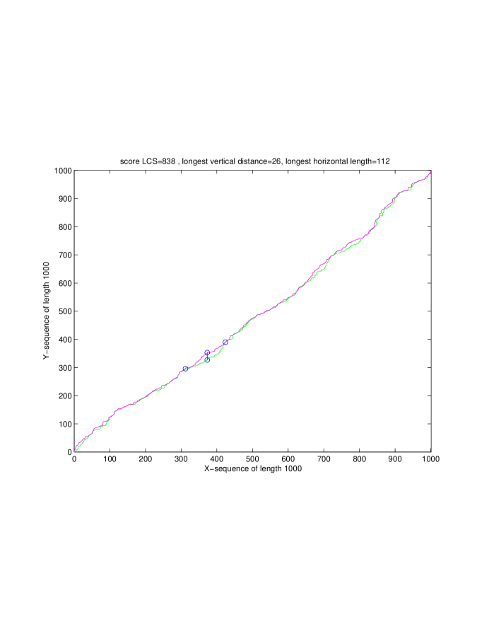
Figure 1: $n=1000$, uniform Bernoulli sequences

Figure 1 is the graph of a simulation with two iid binary sequences of length $n=1000$. All the optimal alignments are contained between the two graphs below and are thus seen to all stay extremely close to the diagonal. The maximal vertical distance between two optimal paths is $26$ and, for this vertical distance, the maximal horizontal stretch between which the two optimal paths split and then meet again is $112$.

5 Short string-lengths properties are generic

Often, a desirable property we want string-pairs to verify, e.g., a similar number of a given symbol or pattern, the presence of dominant matches, only holds with high probability and if the two strings have their lengths not too far away from each other. Moreover, short strings are also often used as “seeds” to find longer or more global similarities and homologous properties ([21] contains many examples of such instances in applied problems). It is our purpose now to attempt to quantify such a generic phenomenon.

To to so, let $\mathcal{P}$ be a relation assigning to every pair of strings $(x,y)$ the value $1$ if the pair $(x,y)$ has a certain property, and $0$ otherwise. Hence, if ${\mathcal{A}}$ is the alphabet we consider,

$$\mathcal{P}:(\cup_{k}\mathcal{A}^{k})\times(\cup_{k}\mathcal{A}^{k})\rightarrow\{0,1\},$$

and if $\mathcal{P}(x,y)=1$, the string pair $(x,y)$ is said to have the property $\mathcal{P}$.

Let now $\epsilon>0$, be fixed, and let $\vec{r}=(r_{0},r_{1},\dots,r_{m})$ satisfy the condition (9). Let also $B^{n}_{\mathcal{P}}(\vec{r},\epsilon)$ be the event that there is a proportion of at least $1-\epsilon$ of the string pairs

$$(X_{(i-1)k+1}\cdots X_{ik};Y_{r_{i-1}+1}\cdots Y_{r_{i}})$$ (50)

satisfying the property $\mathcal{P}$, i.e.,

$$B^{n}_{\mathcal{P}}(\vec{r},\epsilon)=\left\{\sum_{i=1}^{m}\mathcal{P}(X_{(i-1)k+1}....X_{ik};Y_{r_{i-1}+1}\cdots Y_{r_{i}})\geq(1-\epsilon)m\right\}.$$ (51)

Next, let $B^{n}_{\mathcal{P}}(\epsilon)$ be the event that for every optimal alignment the proportion of aligned string pairs (50) satisfying the property $\mathcal{P}$ is at least $1-\epsilon$, i.e., $B^{n}_{\mathcal{P}}(\epsilon)$ holds if and only if for every $\vec{r}=(r_{0},r_{1},\dots,r_{m})$ satisfying (9) and such that $LC_{n}=L_{n}(\vec{r})$, the event $B^{n}_{\mathcal{P}}(\vec{r},\epsilon)$ holds. Finally, assume that as soon as $r_{i}-r_{i-1}\in[kp_{1},kp_{2}]$, the probability that the string-pairs (50) have the required property is at least $1-q$, $q\in[0,1]$. Hence, assume that for every integer $\ell\in[kp_{1},kp_{2}]$:

$$\mathbb{P}\left(\;\mathcal{P}(X_{1}\cdots X_{k};Y_{1}Y_{2}\cdots Y_{\ell})=1\;\right)\geq 1-q.$$

We investigate, now, how small $q=q(k)$ needs to be in order to ensure that a large proportion of the aligned string pairs (50) has the property $\mathcal{P}$ (for every optimal alignment). Recall that $A^{n}_{\epsilon,p_{1},p_{2}}$ is the event that every optimal alignment aligns a proportion of at least $1-\epsilon$ of the sub-strings $X_{(i-1)k+1}\cdots X_{ik}$ with sub-strings of $Y$ with length in $[kp_{1},kp_{2}]$. Recall also that $\mathcal{R}_{\epsilon,p_{1},p_{2}}$ is the set of integer vectors $\vec{r}=(r_{0},r_{1},\dots,r_{m})$, satisfying (9) and such that there is at least $(1-\epsilon)m$ of the differences $r_{i}-r_{i-1}$ in $[kp_{1},kp_{2}]$.

Below, we deal with a small modification of the event $B^{n}_{\mathcal{P}}(\vec{r},\epsilon)$. For this, let $\tilde{B}^{n}_{\mathcal{P}}(\vec{r},\epsilon)$ be the event that among the aligned string pieces (50) there are no more than $m\epsilon$ which do not satisfy the property $\mathcal{P}$ and have their length $r_{i}-r_{i-1}$ in $[kp_{1},kp_{2}]$. Clearly, for $\epsilon_{1}>0$, $\epsilon_{2}>0$,

$$A^{n}_{\epsilon_{1},p_{1},p_{2}}\cap\left(\bigcap_{\vec{r}\in\mathcal{R}_{\epsilon_{1},p_{1},p_{2}}}\tilde{B}^{n}_{\mathcal{P}}(\vec{r},\epsilon_{2})\right)\subset B^{n}_{\mathcal{P}}(\epsilon_{1}+\epsilon_{2}),$$

and so

$$\mathbb{P}((B^{n}_{\mathcal{P}}(\epsilon_{1}+\epsilon_{2}))^{c})\leq\mathbb{P}((A^{n}_{\epsilon_{1},p_{1},p_{2}})^{c})+\sum_{\vec{r}\in\mathcal{R}_{\epsilon_{1},p_{1},p_{2}}}\mathbb{P}((\tilde{B}^{n}_{\mathcal{P}}(\vec{r},\epsilon_{2}))^{c}).$$ (52)

Next,

$$\mathbb{P}((\tilde{B}^{n}_{\mathcal{P}}(\vec{r},\epsilon_{2}))^{c})\leq\binom{m}{\epsilon_{2}m}q^{\epsilon_{2}m}\leq\exp(H_{e}(\epsilon_{2})m)q^{\epsilon_{2}m},$$

where $H_{e}$ is the base $e$ entropy function, given by $H_{e}(x)=-x\ln x-(1-x)\ln(1-x),0<x<1$. Hence,

$$\mathbb{P}((\tilde{B}^{n}_{\mathcal{P}}(\vec{r},\epsilon_{2}))^{c})\leq q^{\epsilon_{2}m}\exp(H_{e}(\epsilon_{2})m).$$ (53)

Using (53) into (52) and, proceeding as in (40), noting that ${\mathcal{R}}_{\epsilon,p_{1},p_{2}}$ has at most $(ek)^{m}$ elements, lead to

$$\mathbb{P}((B^{n}_{\mathcal{P}}(\epsilon_{1}+\epsilon_{2}))^{c})\leq\mathbb{P}((A^{n}_{\epsilon_{1},p_{1},p_{2}})^{c})+(ek)^{m}q^{\epsilon_{2}m}\exp(H_{e}(\epsilon_{2})m).$$ (54)

Taking $q(k)=1/(2ek)^{1/\epsilon_{2}}$, finally yields

$$\mathbb{P}((B^{n}_{\mathcal{P}}(\epsilon_{1}+\epsilon_{2}))^{c})\leq\mathbb{P}((A^{n}_{\epsilon_{1},p_{1},p_{2}})^{c})+\exp(\left(H_{e}(\epsilon_{2})-\ln 2)m\right).$$ (55)

But, for $\epsilon_{2}<1/2$, $H_{e}(\epsilon_{2})<\ln 2$, and then $\exp(\left(H_{e}(\epsilon_{2})-\ln 2)m\right)$ is exponentially small in $m$. Now, our main theorem provides an exponentially small lower bound on $\mathbb{P}((A^{n}_{\epsilon_{1},p_{1},p_{2}})^{c})$. Therefore, (55) asserts that a high proportion of the aligned string pairs (50) has property $\mathcal{P}$, in any optimal alignment, as soon as for pairs (50) with similar length, $q(k)\leq{1}/{(2ek)^{1/\epsilon_{2}}}$, where

$$q(k):=\max_{\ell\in[kp_{1},kp_{2}]}\mathbb{P}(\text{the pair }(X_{1}\cdots X_{k};Y_{1}\cdots Y_{\ell})\text{ does not satisfy property }\mathcal{P}).$$

These assertions are summarized in the next theorem, which is obtained by letting, above, $\epsilon_{1}=\epsilon_{2}=\epsilon/2$, using also Theorem 2.3.

Theorem 5.1.

Let $0<\epsilon<1$. Let $0<p_{1}<1<p_{2}$ be such that $\tilde{\gamma}(p_{1})<\gamma^{*}$ and $\tilde{\gamma}(p_{2})<\gamma^{*}$, and let $0<\delta<\min\left(\gamma^{*}-\tilde{\gamma}(p_{1}),\gamma^{*}-\tilde{\gamma}(p_{2})\right)$. Finally, let the integer $k\geq 1$ be such that

$$\max_{\ell\in[kp_{1},kp_{2}]}\mathbb{P}((X_{1}\cdots X_{k};Y_{1}\cdots Y_{\ell})\text{ does not satisfy property $\mathcal{P}$})\leq\frac{1}{(2ek)^{2/\epsilon}}.$$

Then, for any optimal alignment $\vec{r}$ (i.e., such that $LC_{n}=L_{n}(\vec{r})$), the proportion of string pairs $(X_{(i-1)k+1}\cdots X_{ik};Y_{r_{i-1}+1}\cdots Y_{r_{i}})$ satisfying property $\mathcal{P}$ is at least $1-\epsilon$ with probability at least equal to:

$$1-\mathbb{P}((A^{n}_{\epsilon/2,p_{1},p_{2}})^{c})-\exp\left(\left(H_{e}\left(\frac{\epsilon}{2}\right)-\ln 2\right)m\right),$$

and thus at least equal to:

$$1-\exp\left(-n\left(-\frac{1+\ln k}{k}+\frac{\delta^{2}\epsilon^{2}}{64}\right)\right)-\exp\left(\frac{n}{k}\left(H_{e}\left(\frac{\epsilon}{2}\right)-\ln 2\right)\right),$$

for all $n=n(\epsilon,\delta)$ large enough.

Hence, from the above statement, the probability that less than a proportion $1-\epsilon$ of string pairs (50) have property $\mathcal{P}$ in every optimal alignment is exponentially small in $n$ (while holding $k$, $\epsilon$ and $\delta$ fixed) as soon as

$$k>\frac{64(1+\ln k)}{\epsilon^{2}\delta^{2}},$$ (56)

and

$$\max_{\ell\in[kp_{1},kp_{2}]}\mathbb{P}((X_{1}\cdots X_{k};Y_{1}\cdots Y_{\ell})\;\text{does not satisfy property $\mathcal{P}$})\leq\frac{1}{(2ek)^{2/\epsilon}}.$$ (57)

The above theorem is very useful for showing that when a property holds for aligned string pairs with similar lengths, say of order $k$, then the property typically holds in most parts of the optimal alignment. From our experience, for most properties one is interested in, such as the study of dominant matches in optimal alignments, when $p_{1}$ and $p_{2}$ are close to $1$, but fixed, then the probability that

$$(X_{1}\cdots X_{k};Y_{1}Y_{2}\cdots Y_{\ell})$$

does not satisfy this property is approximately the same for all $\ell\in[kp_{1},kp_{2}]$. In other words, the behavior of the alignment of $X_{1}\cdots X_{k}$ with $Y_{1}\cdots Y_{\ell}$, does not depend much on $\ell$ as soon as $\ell$ is close to $k$ and $k$ is fixed. From (57), what is needed there is a bound, on the left hand-side probability, smaller than any inverse polynomial-order in $k$. (At least to be able to take $\epsilon$ as close to $0$ as one wants to.) If instead $\epsilon>0$ is chosen small but fixed, then an inverse polynomial bound with a very large exponent will do). So, if this probability is, for example, of order $k^{-\ln k}$ or $e^{-k^{\alpha}}$ for some constant $\alpha>0$, the condition (57) is satisfied by taking $k$ large enough. Similarly, condition (56) is always satisfied for $k$ large enough.

We could also envision using Monte Carlo simulation to find a bound for the probability on the left of (57). For that purpose, assume that $\epsilon=0.2$ and take $\delta=0.1$. Then, by (56), $k$ must be at least $2518253$. The probability that strings of length approximately $k$ do not satisfy property $\mathcal{P}$ must be at most $(2ek)^{-10}\approx(13690642)^{-10}$, so a probability smaller than $10^{-70}$. However, this is hardly feasible, indeed, to show that a probability is as small as $10^{-70}$, one would need to run an order of $10^{70}$ simulations.

Further Improvements

There are several ways to improve our various bounds. First, we took as upper bound for cardinality of $\mathcal{R}_{\epsilon,p_{1},p_{2}}$ the value $\binom{n}{m}$, which can be improved as follows: first note that if $\vec{r}=(r_{0},r_{1},\dots,r_{m})\in\mathcal{R}_{\epsilon,p_{1},p_{2}}$, then at least $(1-\epsilon)m$ of the lengths $r_{i+1}-r_{i}$ are in the interval $[kp_{1},kp_{2}]$. To determine these lengths we have at most

$$((p_{2}-p_{1})k)^{m}$$ (58)

choices. Then, there can be as many as $\epsilon m$ of the lengths $r_{i+1}-r_{i}$, which are not in $[kp_{1},kp_{2}]$. Choosing those lengths is like choosing at most $\epsilon m$ points from a set of at most $n$ elements. Hence, we get as upper bound $\binom{n}{\epsilon m}$ which, in turn, can be upper bounded by, say,

$$\left(\frac{ek}{\epsilon}\right)^{\epsilon m},$$ (59)

or via the entropy bound $\exp(nH_{e}(\epsilon/k))$. Finally, we have to decide which among the $m$ lengths $r_{i}-r_{i-1}$ have their length in $[kp_{1},kp_{2}]$ and which have not. That choice is further bounded via:

$$\binom{m}{\epsilon m}\leq\exp(H_{e}(\epsilon)m).$$ (60)

Combining the bounds (58), (59) and (59), yields

$${\rm Card}\left(\mathcal{R}_{\epsilon,p_{1},p_{2}}\right)\leq\left((p_{2}-p_{1})k\left(\frac{ek}{\epsilon}\right)^{\epsilon}\exp(H_{e}(\epsilon))\right)^{m}$$ (61)

With this better bounding for the cardinality of $\mathcal{R}_{\epsilon,p_{1},p_{2}}$, the inequality (54) becomes:

$$\mathbb{P}((B^{n}_{\mathcal{P}}(\epsilon_{1}+\epsilon_{2}))^{c}) \leq\mathbb{P}((A^{n}_{\epsilon_{1},p_{1},p_{2}})^{c})$$

$$\quad+\left((p_{2}-p_{1})k\left(\frac{ek}{\epsilon_{1}}\right)^{\epsilon_{1}}\exp(H_{e}(\epsilon_{1}))\right)^{m}q^{\epsilon_{2}m}\exp(H_{e}(\epsilon_{2})m),$$ (62)

which when combined with Theorem 2.3 yields that

$$\mathbb{P}((B^{n}_{\mathcal{P}}(\epsilon_{1}+\epsilon_{2}))^{c}) \leq\exp\left(-n\left(-\frac{1+\ln k}{k}+\frac{\delta^{2}\epsilon_{1}^{2}}{16}\right)\right)$$

$$\quad+\left((p_{2}-p_{1})k\left(\frac{ek}{\epsilon_{1}}\right)^{\epsilon_{1}}\exp(H_{e}(\epsilon_{1}))q^{\epsilon_{2}}\exp(H_{e}(\epsilon_{2}))\right)^{m}.$$ (63)

Again, this last expression is exponentially small in $n$ (assuming $k$ fixed) if the following two conditions are satisfied:

(i)

$$k>\frac{16(1+\ln k)}{\epsilon_{1}^{2}\delta^{2}},$$ (64)

(the smallest integer $k$ satisfying (64) with $\epsilon_{1}=0.2$ and $\delta=0.1$ is now $570146$) and (ii)

$$q(k)<\frac{1}{\left((p_{2}-p_{1})k\left(\frac{ek}{\epsilon_{1}}\right)^{\epsilon_{1}}\exp(H_{e}(\epsilon_{1})+H_{e}(\epsilon_{2}))\right)^{1/\epsilon_{2}}};$$ (65)

and combining these last two conditions yields:

$$q(k)<\left(\frac{\epsilon_{1}^{2}\delta^{2}}{(p_{2}-p_{1})16(1+\ln k)\left(\frac{ek}{\epsilon_{1}}\right)^{\epsilon_{1}}\exp(H_{e}(\epsilon_{1})+H_{e}(\epsilon_{2}))}\right)^{1/\epsilon_{2}}.$$ (66)

Typically $\epsilon_{1}+\epsilon_{2}$ should be of a given order. So, let us maximize the right-hand side of (66) under the constraint $\epsilon=\epsilon_{1}+\epsilon_{2}$. To do so, note that the power $1/\epsilon_{2}$ has a much more minimizing influence than the expression $\epsilon_{1}^{2}$ in the numerator, while $1\leq\exp(H_{e}(\epsilon_{1})+H_{e}(\epsilon_{2}))\leq 2$ and so this last quantity does not have much of an influence. Also, note $(ek/\epsilon_{1})^{\epsilon_{1}}$ is somewhat negligible compared to $ek$. So, at first, let us disregard the quantities $(ek/\epsilon_{1})^{\epsilon_{1}}$ and $\exp(H_{e}(\epsilon_{1}))+H_{e}(\epsilon_{2}))$, and let

$$g(k,\epsilon_{1},\epsilon_{2}):=\left(\frac{\epsilon_{1}^{2}\delta^{2}}{(p_{2}-p_{1})16(1+\ln k)}\right)^{1/\epsilon_{2}}.$$

Clearly, $g(k,\epsilon_{1},\epsilon_{2})$ is larger than the bound on the right-hand side of (66) and when all the parameters $p_{1},p_{2}$ and $\delta$ are held fixed, $g(k,\epsilon_{1},\epsilon_{2})$ is decreasing in both $\epsilon_{1}$ and $\epsilon_{2}$. However, $\epsilon_{2}$ “has more decreasing influence” than $\epsilon_{1}$. Therefore, given $\epsilon$ and given that all the parameters are fixed (including $k$), maximizing $g(k,\epsilon_{1},\epsilon_{2})$ under the constraint $\epsilon_{1}+\epsilon_{2}=\epsilon$, $\epsilon_{1},\epsilon_{2}>0$ lead to a quantity where $\epsilon_{2}$ is quite a bit larger than $\epsilon_{1}$.

Could Monte Carlo simulations be realistic with $\epsilon=0.1$ and the bounds which we have? The answer is no. Indeed, at first, $\delta/(p_{2}-p_{1})$ gets better when $|p_{2}-p_{1}|$ increases since the derivative of $\tilde{\gamma}$ at $p=1$ is zero. When the interval $[kp_{1},kp_{2}]$ becomes too large however, then the property might no longer hold with high probability for all pairs $(X_{1}\cdots X_{k},Y_{1}\cdots Y_{\ell})$, with $\ell\in[kp_{1},kp_{2}]$. So, we will take $[p_{1},p_{2}]$, as large as possible, so this property still holds with high probability for all the string pairs mentioned before. With such a choice, $\delta/(p_{2}-p_{1})$ can be treated as a constant. Somewhat, optimistically, say that the constant is less than $1/3$. Now if $\epsilon=0.1$, then $\epsilon_{1},\epsilon_{2}\leq 0.1$. In that case,

$$g(k,\epsilon_{1},\epsilon_{2})\leq g(k,0.1,0.1)\leq\left(\frac{0.01\delta}{3\times 16(1+\ln k)}\right)^{10}.$$

Returning to $\eqref{k}$ and taking $\delta=0.2$, we find that $k$ must be larger than $10^{10}$, so that $\ln k$ is bigger than $20$. With this in mind, and in the present case where $\epsilon_{1}+\epsilon_{2}=0.1$, we find that $g(k,\epsilon_{1},\epsilon_{2})$ is smaller $10^{-56}$, so there is still little hope to perform Monte Carlo simulation here.

Monte Carlo simulation with $\epsilon_{1}=0.1$ and $\epsilon_{2}=0.2$: Take also $\delta=0.2$ and $\delta/(p_{2}-p_{1})=1/2$. With these values, and using (64), then $k$ must be somewhat larger than ${10}^{2}\cdot 10\cdot 8\ln(24000)\approx 10^{5}$. Then, by (65), $q(k)$ should also be less than

$$\left(10^{2}\cdot 10\cdot 11\cdot 8\right)^{-5}\approx 10^{-25}.$$

This is still a difficult order for Monte Carlo simulation and if we had $\epsilon_{2}=0.3$ instead, then we would get a bound $10^{-15}$ which remains a difficult order.

When only dealing with the inequality (65), things look somewhat better. Take $k=1000$ and $(p_{1}-p_{1})k=100$, then the bound on $q(k)$ is of order about $10^{-5}$ which is feasible with Monte Carlo. So, if we could find another method than the one described here to make sure that most of the pieces of strings $X_{(i-1)k+1}X_{(i-1)k+2}\cdots X_{ik}$ are aligned with pieces of similar length we would end up in a favorable setting.

Acknowledgments: Many thanks to the referee for a thoughtful and detailed reading of this manuscript.

References

• [1] Alexander, K. S. The rate of convergence of the mean length of the longest common subsequence, Annals of Applied Probability 4, (1994), 1074–1082.
• [2] Amsalu, S., Houdré, C. and Matzinger, H., Sparse long blocks and the micro-structure of the longest common subsequences in random words, J. Stat. Phys., 154, 6, (2014), 1516–1549.
• [3] Amsalu, S., Houdré, C. and Matzinger, H., Sparse long blocks and the variance of the length of the longest common subsequences in random words, ArXiv #math.PR/1204.1009, (2012).
• [4] Baik, J., Deift, P. and Johansson, K. On the distribution of the length of the longest increasing subsequence of random permutations. J. Amer. Math. Soc., 12(4):1119–1178, 1999.
• [5] Breton, J.-C. and Houdré, C., On the limiting law of the length of the longest common and increasing subsequences in random words. ArXiv #Math.PR/1505-06164, (2015).
• [6] Capocelli, R.M., Sequences: Combinatorics, Compression, Security, and Transmission, Springer-Verlag New York, (1989).
• [7] R. Durbin, S.R. Eddy, A. Krogh, and G. Mitchison. Biological Sequence Analysis: Probabilistic Models of Proteins and Nucleic Acids, Cambridge University Press, 1998.
• [8] Chvátal, V. and Sankoff, D., Longest common subsequences of two random sequences, J. Appl. Probability, 12, (1975), 306–315.
• [9] Houdré, C. and Işlak, Ü., A central limit theorem for the length of the longest common subsequences in random words, ArXiv:#math.PR/1408.1559v3, (2015).
• [10] Houdré, C., Lember, J. and Matzinger, H., On the longest common increasing binary subsequence, C.R. Acad. Sci. Paris Ser. I 343, (2006), 589–594.
• [11] Houdré, C. and Litherland, T. L. On the longest increasing subsequence for finite and countable alphabets. HDPV: The Luminy Volume, IMS Collection, 5:185–212, 2009.
• [12] Houdré, C. and Litherland, T. L. On the limiting shape of Young diagrams associated with Markovian random words. ArXiv #math.PR/1110.4570, (2011).
• [13] Houdré, C. and Ma, J., On the order of the central moments of the length of the longest common subsequences in random words, To appear: Progress in Probability: Birkhauser (2016).
• [14] Houdré, C. and Matzinger, H., On the variance of the optimal alignments score for binary random words and an asymmetric scoring function, Under Revision: J. Stat. Phys (2016).
• [15] Its, A. R., Tracy, C. and Widom, H. Random words, Toeplitz determinants, and integrable systems. I. Random matrix models and their applications. Math. Sci. Res. Inst. Publ., 40, 2001.
• [16] Its, A. R., Tracy, C. and Widom, H. Random words, Toeplitz determinants, and integrable systems. II. Advances in nonlinear mathematics and science. Phys. D, 152–153:199–224, 2001.
• [17] Johansson, K. Transversal fluctuations for increasing subsequences on the plane, Probab. Theory Related Fields 116, (2000) 445–456.
• [18] Lember, J. and Matzinger, H., Standard deviation of the LCS when zero and one have different probabilities, Annals of Probability 37, (2009), 1192–1235.
• [19] Lueker, G. S., Improved bounds on the average length of longest common subsequences Journal of the ACM, 56, Art. 17, (2009).
• [20] Robin, S., Rodolphe, F., and Schbath, S., ADN, mots et modèles, Belin, Paris, 2003.
• [21] Sankoff, D., and Kruskal, J., Time warps, string edits and macromolecules: The theory and practice of sequence comparison Center for the Study of Language and Information, 1999.
• [22] Seppäläinen, T., Scaling for a one-dimensional directed polymer with boundary conditions, Ann. Probab. 40, (2012) 19–73.
• [23] Steele, J. M., Long common subsequences and the proximity of two random strings, SIAM J. Appl. Math. 42 (1982), 731–737.
• [24] Waterman, M. S., Estimating statistical significance of sequence alignments Phil. Trans. R. Soc. Lond. B. (1994), 383–390.
• [25] Waterman, M. S., Introduction to Computational Biology: Maps, Sequences and Genomes (Interdisciplinary Statistics), CRC Press (2000).