Transport properties of quantum dots in the Wigner molecule regime

Abstract

The transport properties of quantum dots with up to $N=7$ electrons ranging from the weak to the strong interacting regime are investigated via the projected Hartree-Fock technique. As interactions increase radial order develops in the dot, with the formation of ring and centered-ring structures. Subsequently, angular correlations appear, signalling the formation of a Wigner molecule state.
We show striking signatures of the emergence of Wigner molecules, detected in transport. In the linear regime, conductance is exponentially suppressed as the interaction strength grows. A further suppression is observed when centered-ring structures develop, or peculiar spin textures appear. In the nonlinear regime, the formation of molecular states may even lead to a conductance enhancement.

1 Introduction

Semiconductor quantum dots (QDs), frequently referred to as artificial atoms, are nanometer-sized structures whose conduction electrons are confined in all the three spatial dimensions [1, 2, 3]. In these systems a two-dimensional electron gas, formed at the interface of a heterojunction, is depleted by chemical etching or electrostatic potentials in order to form an isolated region, connected to external reservoirs by tunnel barriers. For a small number of particles $N$, the potential can often be considered as harmonic [1, 2, 3].
In analogy to atomic systems, quantum dots can be probed optically by studying their absorption or emission spectrum [4]. Additionally, the study of transport properties is a source of information for quantum dots embedded into an electronic circuit [1]. The current flow proceeds by tunnelling events once a bias voltage is applied to the external reservoirs and the presence of an external gate voltage allows to tune the number of excess electrons in the dot with respect to a neutral configuration.

Theoretically, the study of correlated quantum dot states is a challenging many-body problem: even the fairly simple case of $N=2$ can be solved exactly only in specific regimes [5], whereas in general one has to resort to semi-analytic methods [6] or approximate WFs [7]. For $N>2$, several numerical methods have been employed. In increasing order of computational complexity they range from unrestricted Hartree-Fock methods [8, 9, 10, 11] and density functional theory [12, 13, 14, 15, 16], to projected Hartree-Fock (PHF) [17, 18, 9, 19, 20, 21, 22, 23], random phase approximation [24, 25], quantum Monte Carlo [16, 26, 27, 28, 29], and exact diagonalization [30, 31, 32, 33, 34, 35, 36, 37, 38, 39]. Recently, PHF techniques have been used by our group for the study of correlated quantum dots. While retaining the flexibility of an unrestricted Hartree-Fock approach, PHF allows to overcome the limitations due to symmetry broken solutions and to efficiently obtain dot wavefunctions (WFs) with the correct spin and angular momentum, showing correlations beyond the mean field level [21, 22].

Circular two-dimensional systems realized e.g. by pillar quantum dots display interesting features depending on the ratio $\lambda$ between the strength of the typical interaction and the strength of the confining potential – see Sec. 2.1 for a precise definition of $\lambda$. When $\lambda$ is small, atomic-like effects due to quantum mechanical confinement such as the formation of shell structures have been observed [40, 41, 42] and explained at the mean field level [1, 43]. For increasing $\lambda$, several numerical investigations have shown the emergence of correlated electron states and the occurrence of Wigner molecular states [44, 33, 34, 36, 37, 38, 39, 45, 26, 8, 32, 18, 46, 10, 47, 48, 49, 50, 35, 51, 19, 52, 53, 27, 28, 29, 54, 55, 56, 57, 58, 12], the finite-size analogue of Wigner crystals [59, 60], characterized by correlations beyond the mean field.
The transition towards a molecular state occurs smoothly [26, 12, 27, 28, 29, 47, 58]. As interactions increase, the dot WFs cross over from weakly correlated states at small $\lambda$ to Wigner molecular states, characterized by strong correlations. The transition occurs in two phases:

• At small $\lambda$, correlations begin to develop and ring-like structures develop in the dot WF. For $N\geq 6$, also centered structures with one or more electrons in the dot center may form.

• For higher $\lambda$, angular correlations begin to appear as the dot enters the incipient Wigner molecule regime [27, 28]. Increasing $\lambda$ further, the dot WF represents a rotating Wigner molecule [45] and the electrons localize around the equilibrium positions of a classical Coulomb molecule [44, 49].

Correlations are particularly relevant also in one-dimensional systems which display an analogous transition towards the Wigner molecule [61, 62, 63, 64, 65].
The experimental observation of strongly correlated states in quantum dots has attracted considerable interest. In pillar quantum dots, inelastic light scattering experiments have shown signatures of correlated quantum states [57, 66]. Scanning tunnelling spectroscopy experiments for the imaging of correlated quantum dot WFs were recently performed and theoretically analyzed [55, 56, 67]. Also transport properties can yield information about correlated states. In one dimension, the influence of correlations on the transport properties is predicted to be particularly important [68, 69, 70]. Recently, experimental evidence of the formation of few-electrons Wigner molecules has been reported in carbon nanotubes [71].

Also spin correlations can heavily influence the transport properties of quantum dots, even in the absence of an applied magnetic field. In quantum dots with asymmetric tunnel barriers, the degeneracy of spin multiplets may lead to asymmetric current-voltage characteristics [72]. Another notable example is the type-II spin blockade [73, 74], which occurs in the linear transport regime when the absolute value of the difference between the total spin of initial and final dot states exceeds 1/2 and leads to zero sequential current through the dot.

In this paper we investigate the transport properties of quantum dots in the presence of strong correlations. In such a regime, a mean field treatment in the spirit of the so called “constant interaction model” [40, 75] is clearly not viable. Indeed, one has to resort to more precise techniques to obtain the spectrum and the WFs. Numerical studies of the transport properties, similar to the one proposed here have been performed in the past employing exact diagonalizations for $N\leq 3$ electrons in circular QDs [76, 77, 78] and $N\leq 4$ electrons in one-dimensional quantum dots [79]. These works, however, were not focused on the signatures due to Wigner molecules in the transport properties.

In the present work we numerically investigate the transport properties of pillar quantum dots beyond the constant interaction model. Our model is that of $N$ interacting electrons confined to a two-dimensional plane and further subject to an in-plane harmonic potential. More refined models, including effects due to a finite thickness of the dot and to heavy doping in the reservoirs, have been recently proposed [80]. In this work we will neglect such effects, addressing systems in which the screening is moderate (a strong screening may hinder the formation of Wigner molecules [61, 81]). We use the PHF method in order to estimate the correlated dot WFs for $4\leq N\leq 7$ in a range of $\lambda$ which allows to observe the transition between liquid-like and molecular electron states. Sequential tunnelling rates are numerically evaluated and the dot conductance is obtained using a rate equation.

Our task is to understand whether or not peculiar signatures in the transport properties may be detected as a consequence of the transition towards the Wigner molecule. According to the results presented in this paper, the answer is affirmative.

In the linear transport regime, qualitative modifications of the dot ground state (GS) WFs induce a peculiar suppression of the conductance. Such qualitative modifications may be induced either by the formation of centered ring-like structures or by the emergence of peculiar spin patterns in the dot WF. Both cases are presented in this paper.
Signatures of the transition can also be seen in the nonlinear transport regime. We have found that the tunnelling rate through an excited state of the dot may be increased strongly by the formation of a Wigner molecule.
The features described above are genuine hallmarks of the formation of Wigner molecules in the dot and can be expected to be observable in experiments.

The outline of the paper is as follows. In Sec. 2 we introduce the model and the PHF method, we discuss the tunnelling Hamiltonian and the rate equation for calculating the current. Results are presented in Sec. 3. Here, after discussing in detail the occurrence of Wigner molecules, we show results for the conductance in both the linear and nonlinear regimes. Conclusions are presented in Sec. 4. A contains the derivation of the tunnelling Hamiltonian while the dot tunnelling rates are discussed in B.

2 Model and methods

2.1 Quantum dot

In a pillar quantum dot [40, 41, 42, 43] electrons are confined to a thin disk of semiconducting material, represented by the red region in figure 1. The dot is embedded between tunnel barriers located around $z=z_{\mathrm{E}},z_{\mathrm{C}}$, with $z$ the axial direction. The tunnel barriers couple the dot to the external emitter and collector contacts [2]. A metallic gate is assumed to surround the dot region (not shown in figure 1) and allows to shift the dot energy levels as a suitable gate voltage $V_{\mathrm{g}}$ is applied to it.

Figure 1: Schematic representation of a pillar quantum dot. The red thin disc is the quantum dot (D), connected via tunneling barriers at $z\approx z_{\mathrm{E}},z_{\mathrm{C}}$ (yellow parts) to emitter (E) and collector (C) leads, represented in blue.

Due to the strong confinement along $z$, the motion of electrons is essentially restricted to the $(x,y)$ plane. Electrons are further subject to a lateral confining potential with rotational symmetry around the $z$ axis, as appropriate for the cylindrical quantum dots studied in this paper. For small dots, containing few electrons, this potential is well approximated by a parabolic one [2]. The Hamiltonian for $N$ interacting electrons is $\hat{H}_{\mathrm{D}}=\hat{H}_{\mathrm{D}}^{(0)}+\hat{H}_{\mathrm{D}}^{(1)}$ with ($\hbar=1$, boldface denotes vectors)

$$\hat{H}_{\mathrm{D}}^{(0)}=\sum_{i=1}^{N}\left[\frac{1}{2m^{*}}\hat{{\mathbf{P}}}_{i}^{2}+\frac{m^{*}\omega^{2}}{2}\hat{{\mathbf{R}}}_{i}^{2}\right]-eNV_{\mathrm{g}}\ \ ;\ \ \hat{H}_{\mathrm{D}}^{(1)}=\frac{e^{2}}{4\pi\varepsilon_{0}\varepsilon_{{\mathrm{r}}}}\sum_{i=1}^{N-1}\sum_{j=i+1}^{N}\frac{1}{|\hat{\mathbf{R}}_{i}-\hat{\mathbf{R}}_{j}|}\,,$$ (1)

where $\hat{\mathbf{R}}_{i}=(\hat{x}_{i},\hat{y}_{i})$ is the $i$-th electron coordinate and $\hat{\mathbf{P}}_{i}$ its momentum. Here, $-e$ and $m^{*}$ are the electron charge and effective mass respectively. Furthermore, $\omega$ is the confinement energy, $\varepsilon_{0}$ ($\varepsilon_{\rm r}$) the vacuum (relative) dielectric constant. We will consider a bare Coulomb potential for the interaction term $\hat{H}_{\mathrm{D}}^{(1)}$, neglecting both finite-thickness effects and screening due to heavily doped contacts. Such effects modify the interaction potential producing deviations from the $r^{-1}$ behaviour for both short and long inter-electron distances $r$ [80]. Finite thickness effects would also produce a renormalization of the gate voltage $V_{\mathrm{g}}$ [80]. Our calculations are therefore valid for systems characterized by weak screening.
Expressing lengths in units of $\ell_{0}=(m^{*}\omega)^{-1/2}$ and energies in units $\omega$, the Hamiltonian becomes

$$\hat{H}_{\mathrm{D}}^{(0)}=\sum_{i=1}^{N}\left[\frac{\hat{{\mathbf{p}}}_{i}^{2}}{2}+\frac{\hat{{\mathbf{r}}}_{i}^{2}}{2}\right]-\frac{eV_{\mathrm{g}}}{\omega_{0}}N\quad;\quad\hat{H}_{\mathrm{D}}^{(1)}=\lambda\sum_{i=1}^{N-1}\sum_{j=i+1}^{N}\frac{1}{|\hat{\mathbf{r}}_{i}-\hat{\mathbf{r}}_{j}|}\,,$$ (2)

with $\hat{\mathbf{r}}_{i}=\hat{\mathbf{R}}_{i}/\ell_{0}$ and $\hat{\mathbf{p}}_{i}=\hat{\mathbf{P}}_{i}\ell_{0}$. The dimensionless parameter

$$\lambda=\frac{e^{2}}{4\pi\varepsilon_{0}\varepsilon_{\rm r}\ell_{0}\omega}=\frac{\ell_{0}}{a_{\mathrm{B}}^{*}}$$ (3)

measures the Coulomb interaction strength. It is the ratio between the effective length scale $\ell_{0}$ and the effective Bohr radius $a_{\mathrm{B}}^{*}=4\pi\varepsilon_{0}\varepsilon_{\rm r}/m^{*}e^{2}$. Experimentally, the interaction strength $\lambda$ can be modified by tuning the confinement strength $\omega$ via electrostatic gates.
In the rest of the paper, we will concentrate on GaAs quantum dots, where $\varepsilon_{\mathrm{r}}=12.4$ and $m^{*}=0.067m_{\mathrm{e}}$ with $m_{\mathrm{e}}=9.1\cdot 10^{-31}$ kg. In this case, expressing $\omega$ in meV, one has $\lambda\approx 3.46\ \sqrt{\mathrm{meV}}/\sqrt{\omega}$. Weak (strong) interactions occur for $\lambda\lesssim 1$ ($\lambda>1$). In the absence of interactions ($\lambda=0$) the problem can be solved exactly [82]. The eigenstates of $\hat{H}_{\mathrm{D}}^{(0)}$ are Fock-Darwin (FD) states labelled by a principal quantum number $n\geq 0$, by the electron angular momentum ($z$ component) $l\in\mathbb{Z}$ and by the electron spin $z$ component $s_{z}=\pm 1/2$. The corresponding WFs are denoted by $f_{n,l,s_{z}}(\mathbf{r})$ and the spin degenerate energy spectrum is given by $E_{n,l,s_{z}}=\omega(2n+|l|+1)$. In the presence of interactions, the problem cannot be tackled analytically if $N>2$ and one has to use numerical techniques. It is important to notice the symmetries of $\hat{H}_{\mathrm{D}}$: it commutes with the total angular momentum ($z$ component) $\hat{L}$, the total spin $\hat{\mathbf{S}}$ and the total spin $z$ component $\hat{S}_{z}$. As a consequence, their eigenvalues can be used to label the dot energy spectrum and WFs. These are obtained by means of the PHF technique which has been extensively described in [21, 22]. Here, we briefly outline the procedure. For a given particle number $N$ and each value of $-N/2\leq S_{z}\leq N/2$, the dot WFs are first approximated as single Slater determinants $|N,S_{z}\rangle$ made up of $N_{\uparrow}$ ($N_{\downarrow}$) orbital with spin $s_{z}=1/2$ ($s_{z}=-1/2$) where $S_{z}=(N_{\uparrow}-N_{\downarrow})/2$ and $N=N_{\uparrow}+N_{\downarrow}$. Orbitals are variationally optimized with the spin and spatially unrestricted Hartree-Fock method [8] which produces several stationary states $|N,S_{z}\rangle_{i}$, in general neither eigenstates of $\hat{L}$, nor of $\hat{S}^{2}$. Projection operators $\hat{P}_{L,S}$ are subsequently applied to $|N,S_{z}\rangle_{i}$ to restore the symmetries broken due to the single Slater determinant ansatz. As a result, correlated WFs

$$|N,L,S,S_{z}\rangle_{i}=\hat{P}_{L,S}|N,S_{z}\rangle_{i}$$

are obtained. The state in (2.1) cannot be represented as a single Slater determinant and contains correlations beyond mean field. The dot ground state is obtained as the state which minimizes the energy

$$E_{N,L_{0},S_{0},S_{z0}}=\min_{L,S,S_{z},i}\left\{\frac{\leftidx{{}_{i}}{\langle N,S_{z}|}\hat{H}\hat{P}_{L,S}|N,S_{z}\rangle_{i}}{\leftidx{{}_{i}}{\langle N,S_{z}|}\hat{P}_{L,S}|N,S_{z}\rangle_{i}}\right\}\,.$$ (4)

Here, $L_{0}$, $S_{0}$, $S_{z0}$ is the set of quantum numbers which minimize (4) and which label the dot ground state for $N$ electrons, with WF $|N,L_{0},S_{0},S_{z0}\rangle$. In a similar fashion one defines excited states within the PHF method. For instance, the first excited state is given by

$$E_{N,L_{1},S_{1},S_{z1}}=\min_{L,S,S_{z},i}\left\{\frac{\leftidx{{}_{i}}{\langle N,S_{z}|}\hat{H}\hat{P}_{L,S}|N,S_{z}\rangle_{i}}{\leftidx{{}_{i}}{\langle N,S_{z}|}\hat{P}_{L,S}|N,S_{z}\rangle_{i}}>E_{N,L_{0},S_{0},S_{z0}}\right\}\,,$$ (5)

with $L_{1}$, $S_{1}$, and $S_{z1}$ determined by the minimization procedure. As a consequence of the correlations introduced by the projection technique, energies lower than those obtained by unrestricted Hartree-Fock are achieved [21, 22].

2.2 Tunnelling rates

As shown in A, assuming cylindrical symmetry about the $z$ axis and separability of longitudinal and transverse motions, the tunnelling Hamiltonian between the quantum dot and the leads is [83]

$$\hat{H}_{\mathrm{t}}=\sum_{\alpha=\mathrm{E,C}}\sum_{\xi_{\alpha},\eta}\tau_{\xi_{\alpha},\eta}^{(\alpha)}\hat{c}_{\alpha,\xi_{\alpha}}^{\dagger}\hat{d}_{\eta}+\mathrm{h.c.}$$ (6)

where $\alpha={\mathrm{E}}$ ($\alpha={\mathrm{C}}$) for the emitter (collector), $\xi_{\alpha}$ and $\eta$ collectively denote a set of single particle quantum numbers for the lead $\alpha$ and the dot respectively and $\tau_{\xi_{\alpha},\eta}^{(\alpha)}$ is the tunnelling amplitude. In the following, we will choose the FD states $\eta=\left\{n_{\eta}^{(\mathrm{D})},l_{\eta}^{(\mathrm{D})},s_{z\eta}^{(\mathrm{D})}\right\}$ as a basis of single particle states for the dot. In the case of a pillar quantum dot one obtains $\tau_{\xi_{\alpha},\eta}\approx t^{(\alpha)}\delta_{\nu_{\alpha},\eta}$, see (27). The choice of FD states is not restrictive: indeed every orthonormal and complete basis for the single particle states of the dot produces identical results, as shown in C. The fermionic operator for the lead $\alpha$ is $\hat{c}_{\alpha,\xi_{\alpha}}$, while $\hat{d}_{\eta}$ is the one for the dot. Leads are treated as noninteracting Fermi gases with the Hamiltonian

$$\hat{H}_{\alpha}=\sum_{\xi_{\alpha}}E_{\alpha}(\xi_{\alpha})c_{\alpha,\xi_{\alpha}}^{\dagger}c_{\alpha,\xi_{\alpha}}\,,$$ (7)

with energy spectrum $E_{\alpha}(\xi_{\alpha})$.
Our task is to evaluate the sequential tunnelling rates between initial ($|\mathcal{I}_{\mathrm{D}}\rangle$) and final ($|\mathcal{F}_{\mathrm{D}}\rangle$) dot states with energies $E_{{\mathcal{I}}_{\mathrm{D}}}$ and $E_{{\mathcal{F}}_{\mathrm{D}}}$, respectively. As shown in B, the rates are obtained by tracing out the degrees of freedom of the leads, and have the general form

$$\Gamma_{\mathcal{I}_{\mathrm{D}}\to\mathcal{F}_{\mathrm{D}}}=\sum_{\alpha=\mathrm{E,C}}\sum_{p=\pm 1}\Gamma_{\mathcal{I}_{\mathrm{D}}\to\mathcal{F}_{\mathrm{D}}}^{(\alpha),p}\,,$$ (8)

where $p=+1$ ($p=-1$) represents tunnelling into (out from) the dot via lead $\alpha$. They are

$$\Gamma_{\mathcal{I}_{\mathrm{D}}\to\mathcal{F}_{\mathrm{D}}}^{(\alpha),p}=\Gamma^{(\alpha)}\left|\mathcal{O}_{p}\right|^{2}f_{p}(\mu_{\mathrm{D}}-\mu_{\alpha})\,,$$ (9)

where $\Gamma^{(\alpha)}=2\pi\mathcal{D}_{\alpha}|t^{(\alpha)}|^{2}$ is the bare tunnelling rate with $\mathcal{D}_{\alpha}$ the density of states of lead $\alpha$ and $f_{p}(E)=pf(E)+(1-p)/2$, where $f(E)=[1+\exp(\beta E)]^{-1}$ is the Fermi distribution at inverse temperature $\beta=1/k_{\mathrm{B}}T$ ($k_{\mathrm{B}}$ the Boltzmann constant). The chemical potential of the dot is $\mu_{\mathrm{D}}=E_{{\mathcal{F}}_{\mathrm{D}}}-E_{{\mathcal{I}}_{\mathrm{D}}}$ and those for the leads are $\mu_{\alpha}=\mu_{0}+\delta\mu_{\alpha}$. Here, $\delta\mu_{\alpha}$ is a shift due to the presence of a bias voltage $V$. In the following, symmetric voltage drops will be assumed at the barriers, with $\delta\mu_{\mathrm{E}}=eV/2$ and $\delta\mu_{\mathrm{C}}=-eV/2$.
Interaction effects are embodied into the term

$$\mathcal{O}_{1}=\sum_{\eta}\langle\mathcal{F}_{\mathrm{D}}|\hat{d}_{\eta}^{\dagger}|\mathcal{I}_{\mathrm{D}}\rangle\quad;\quad\mathcal{O}_{-1}=\sum_{\eta}\langle\mathcal{F}_{\mathrm{D}}|\hat{d}_{\eta}|\mathcal{I}_{\mathrm{D}}\rangle\,,$$ (10)

which can be evaluated numerically once the initial and the final dot states have been obtained by means of PHF. For $\lambda=0$, one can only have $|\mathcal{O}_{p}|^{2}=0,1$ depending on the initial and final dot states. For $\lambda>0$, on the other hand, $|\mathcal{O}_{p}|^{2}$ is not limited to these two extreme cases. Note that $|\mathcal{O}_{p}|^{2}$ contains interference effects between different FD orbitals.

2.3 Rate equation

Using the tunnelling rates one can set up a rate equation for the occupation probabilities $P_{\mathcal{I}}$ of the dot states $|\mathcal{I}\rangle$ (in this section, we omit the subscript D for simplicity)

$$\frac{\partial{P}_{\mathcal{I}}}{\partial t}=\sum_{\mathcal{J}}M_{\mathcal{I}\mathcal{J}}P_{\mathcal{J}}\,.$$ (11)

The rate equation is a powerful and standard tool to study the transport properties of quantum dots, especially in the sequential regime [75].

The transition matrix $M_{\mathcal{IJ}}$ is defined as

$$M_{\mathcal{I}\mathcal{J}}=\Gamma_{\mathcal{J}\to\mathcal{I}}\left(1-\delta_{N_{\mathcal{I}},N_{\mathcal{J}}}\right)+W_{\mathcal{J}\to\mathcal{I}}\delta_{N_{\mathcal{I}},N_{\mathcal{J}}}\quad\quad \mathrm{if}\ \mathcal{I}\neq\mathcal{J}$$

$$M_{\mathcal{I}\mathcal{I}}=-\sum_{\mathcal{I^{\prime}}\neq\mathcal{I}}M_{\mathcal{I^{\prime}}\mathcal{I}}\,,$$

with $\Gamma_{{\mathcal{J}}\to{\mathcal{I}}}$ given in (8). In order to take into account dissipation effects on the excited states, we introduced a phenomenological relaxation rate

$$W_{\mathcal{I}\to\mathcal{J}}=W\quad\quad \mathrm{if}\ E_{\mathcal{J}}<E_{\mathcal{I}}\,;$$

$$W_{\mathcal{I}\to\mathcal{J}}=W\rme^{-\beta(E_{\mathcal{J}}-E_{\mathcal{I}})}\quad\quad \mathrm{if}\ E_{\mathcal{J}}\geq E_{\mathcal{I}}\,.$$ (12)

In the stationary regime, the left hand side of (11) vanishes and the rate equation reduces to a standard linear system of equations for the stationary occupation probabilities of dot states $\bar{P}_{\mathcal{I}}$ which can be easily solved by means of singular value decomposition since $\det(M_{\mathcal{I}\mathcal{J}})=0$. The solution is uniquely determined by imposing the normalization condition $\sum_{\mathcal{I}}\bar{P}_{\mathcal{I}}=1$. Once the dot occupation probabilities are obtained, the stationary current $I^{(\alpha)}$ through barrier $\alpha$ can be calculated with the aid of the barrier-resolved tunnelling rates (9) as

$$I^{(\alpha)}=e\sum_{\mathcal{I}}\sum_{\mathcal{J}\neq I}\sum_{p=\pm 1}p\bar{P}_{\mathcal{I}}\Gamma_{\mathcal{I}\to\mathcal{J}}^{(\alpha),p}\,.$$ (13)

In the stationary regime, $I^{(\mathrm{E})}=-I^{(\mathrm{C})}=I$. The differential conductance is defined as $\mathcal{G}=\partial I/\partial V$.

2.4 Quasiparticle wavefunction

Useful information about the dot states can also be extracted from the quasiparticle WF (QPWF) [56]

$$\varphi(\mathbf{r})=\sum_{s_{z}=\pm 1/2}\langle\mathcal{F}_{\mathrm{D}}|\hat{\psi}^{\dagger}_{s_{z}}(\mathbf{r})|\mathcal{I}_{\mathrm{D}}\rangle$$ (14)

where

$$\hat{\psi}_{s_{z}}^{\dagger}(\mathbf{r})=\sum_{n\geq 0,l}f_{n,l,s_{z}}^{*}(\mathbf{r})\hat{d}_{n,l,s_{z}}^{\dagger}$$ (15)

is the dot field operator, with $f_{n,l,s_{z}}(\mathbf{r})$ the FD WFs, and the final dot state $|\mathcal{F}_{\mathrm{D}}\rangle$ has one extra electron with respect to the initial one $|\mathcal{I}_{\mathrm{D}}\rangle$. The squared modulus $|\varphi(\mathbf{r})|^{2}$ is proportional to the probability density of tunnelling into the dot at position $\mathbf{r}$.
The QPWF is the analog of the single particle WF of a tunnelling electron for the case of an interacting quantum dot: for $\lambda=0$ it simply reduces to the WF of the FD orbital occupied by the tunnelling electron.
For a transition from the state $|N,L,S,S_{z}\rangle$ to $|N+1,L^{\prime},S^{\prime},S_{z}^{\prime}\rangle$, the QPWF has the general form in polar coordinates ${\mathbf{r}}\to(r,\theta)$ [56]

$$\varphi(r,\theta)=\rme^{\rmi\theta\Delta L}|\varphi(r)|\,,$$ (16)

where $\Delta L=L^{\prime}-L$. Furthermore, $|\varphi(r)|\propto r^{|\Delta L|}$ if $r\to 0$ and $|\varphi(r)|\to 0$ for $r\to\infty$.

3 Results

In this section we present results for a GaAs-based quantum dot with $4\leq N\leq 7$, with parameters $\varepsilon_{\mathrm{r}}=12.4$ and $m^{*}=0.067m_{\mathrm{e}}$ where $m_{\mathrm{e}}=9.1\cdot 10^{-31}$ kg.
For the PHF calculations, we use a truncated basis consisting of 75 FD states per spin direction. Projection operators are numerically implemented with a fast Fourier transform over 256 samples. For further details, see [22]. The ground state and first few excited states are obtained for interaction strengths in the range $1\leq\lambda\leq 2.8$.

3.1 Molecular states of electrons

In table 1 the quantum numbers of the many-body ground states of the dot for increasing values of $\lambda$ are shown as derived from the PHF procedure. Dot states consist of multiplets, degenerate on $S_{z}$ and on $L=\pm L_{0}$.

Table 1: Quantum numbers of the dot GSs as a function of $N$ in the range $1\leq\lambda\leq 2.8$.

• $N$	L	S	$S_{z}$
  4	0	1	0,$\pm 1$
  5	$\pm 1$	1/2	$\pm 1/2$
  6	0	0	0
  7	$\pm 2$	1/2	$\pm 1/2$

Dot quantum numbers are constant throughout the whole range of interaction strengths $1\leq\lambda\leq 2.8$ considered in this paper. They agree with the results of more refined exact diagonalizations [39].
As the interaction strength increases, the dot GS WFs undergo profound modifications, crossing over from weakly correlated states at small $\lambda$ to Wigner molecular states, characterized by strong correlations among electrons, for higher $\lambda$ [26, 12, 27, 28, 29, 47, 58]. The crossover is smooth and occurs through two phases [27, 28, 29].
First, radial correlations begin to develop. As a result, ring-like structures are formed. In addition, for $N\geq 6$ also centered structures appear, with the localization of one or more electrons in the center.
As $\lambda$ is increased, angular correlations begin to develop entering the incipient Wigner molecule regime [27, 28]. Eventually, for strong interactions, the dot WF becomes a rotating Wigner molecule, with electrons localized around positions corresponding to those of classical charged particles parabolically confined [44, 49]. Such states are the analogue of the Wigner crystal [59] but with a finite size. Angular correlations cannot be resolved in a rotationally invariant system but can be characterized by studying two-body angular correlation functions, which show an oscillatory behaviour [27, 28, 29].
Also the WFs calculated with PHF show a behaviour in qualitative agreement to the above results. Let us begin to introduce the spin-resolved one-body electron density $\rho_{1}^{s_{z}}(\mathbf{r})$, defined for a normalized dot state $|N,L,S,S_{\mathrm{z}}\rangle$ as

$$\rho_{1}^{s_{z}}(\mathbf{r})=\langle N,L,S,S_{z}|\hat{\psi}^{\dagger}_{s_{z}}(\mathbf{r})\hat{\psi}_{s_{z}}(\mathbf{r})|N,L,S,S_{z}\rangle$$ (17)

and $\hat{\psi}_{s_{z}}(\mathbf{r})$ defined in (15). In this section we want to illustrate the most relevant aspects of the transition towards the Wigner molecule and will not enter into details about the spin structure of such states. Therefore, we only need to consider the total charge density, summed over the spin:

$$\rho_{1}(\mathbf{r})=\sum_{s_{z}=\pm 1/2}\rho_{1}^{s_{z}}(\mathbf{r})\,.$$ (18)

Since the dot WFs are eigenstates of the angular momentum, introducing polar coordinates $\mathbf{r}\to(r,\theta)$ one has $\rho_{1}(\mathbf{r})\equiv\rho_{1}(r)$.

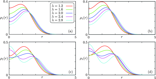
Figure 2: One-body density $\rho_{1}(r)$ (units: $\ell_{0}^{-2}$) of the dot GS as a function of the distance from the dot center $r$, for different interaction strengths $\lambda$ (shown in the inset) and number of particles $N$: (a) $N=4$; (b) $N=5$; (c) $N=6$; (d) $N=7$. For dot parameters, see text. As discussed in Sec. 2.1, here and in the following $r$ is normalized to $\ell_{0}$.

A plot of $\rho_{1}(r)$ for different values of $\lambda$ is represented in figure 2. For $N=4$ and $N=5$, with increasing interactions the density is depleted in the core of the dot and a sharp ridge is formed at its edge, suggesting the formation of a ring-like structure. The position of such ridge moves outwards as the interaction strength increases. Also for $N=6,7$ a ridge develops at the edge and moves outwards for increasing $\lambda$. Additionally, for $N=6$ ($N=7$) the density develops a bump for $r\approx 0$ when $\lambda\gtrsim 2$ ($\lambda\gtrsim 1.8$). This behaviour is consistent with the formation of a centered ring structure. As we shall see in the next section, this latter rearrangement of the WF produces detectable signatures in the transport properties. All these findings show that, for increasing $\lambda$, radial correlations among electrons get more pronounced.
In order to investigate the development of angular correlations and the emergence of a Wigner molecular state, one can introduce the two-body correlation function

$$\!\!\!\!\!\!\!\!\rho_{2}^{s_{z},s_{z}^{\prime}}(\mathbf{r},\mathbf{r}^{\prime})=\langle N,L,S,S_{z}|\hat{\psi}^{\dagger}_{s_{z}}(\mathbf{r})\hat{\psi}^{\dagger}_{s_{z}^{\prime}}(\mathbf{r}^{\prime})\hat{\psi}_{s_{z}^{\prime}}(\mathbf{r}^{\prime})\hat{\psi}_{s_{z}}(\mathbf{r})|N,L,S,S_{z}\rangle\,,$$ (19)

connected to the pair distribution function $g_{s_{z},s_{z}^{\prime}}(\mathbf{r},\mathbf{r}^{\prime})$ by $\rho_{2}^{s_{z},s_{z}^{\prime}}(\mathbf{r};\mathbf{r}^{\prime})=\rho_{1}^{s_{z}}(\mathbf{r})\rho_{1}^{s_{z}^{\prime}}(\mathbf{r}^{\prime})g_{s_{z},s_{z}^{\prime}}(\mathbf{r},\mathbf{r}^{\prime})$ [60]. It is proportional to the conditional probability of finding one electron with spin $s_{z}$ at $\mathbf{r}$, provided that another electron with spin $s_{z}^{\prime}$ is at $\mathbf{r}^{\prime}$. For the qualitative discussion in this section, we consider the total two-body correlation function

$$\rho_{2}(\mathbf{r},\mathbf{r}^{\prime})=\sum_{s_{z}=\pm 1/2}\sum_{s_{z}^{\prime}=\pm 1/2}\rho_{2}^{s_{z},s_{z}^{\prime}}(\mathbf{r},\mathbf{r}^{\prime})\,.$$ (20)

An example of the spin structure of the Wigner molecules will be discussed by employing $\rho_{2}^{s_{z},s_{z}^{\prime}}(\mathbf{r})$ in Sec. 3.2.1, in connection with transport results.
A natural choice for studying $\rho_{2}(\mathbf{r},\mathbf{r}^{\prime})$ is to fix $\mathbf{r}^{\prime}$ at one point on the ridge of the one-body density: $|\mathbf{r}^{\prime}|=r_{0}(N,\lambda)$ and $\theta^{\prime}=0$, where $r_{0}(N,\lambda)$ denotes the position of the off-center maximum of $\rho_{1}(r)$ for $N$ electrons at interaction strength $\lambda$.

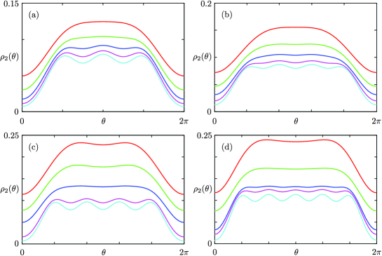
Figure 3: Angular dependence of the two-body density functions $\rho_{2}(\theta)=\rho_{2}(r_{0}(N,\lambda),\theta,r_{0}(N,\lambda),0)$ (units: $\ell_{0}^{-4}$) for the dot GSs for different values of $\lambda$ and (a) $N=4$; (b) $N=5$; (c) $N=6$; (d) $N=7$. Color-codes for $\lambda$ are the same as in figure 2.

Figure 3 shows $\rho_{2}(\theta)=\rho_{2}(r_{0}(N,\lambda),\theta,r_{0}(N,\lambda),0)$ as a function of $\theta$ for different values of $\lambda$. For weak interactions ($\lambda\approx 1$, red and green curves), the correlation function is almost flat except for the “Fermi hole” at $\theta=0,2\pi$, essentially induced by the Pauli exclusion principle. This confirms that correlations among the electrons within the ring are weak. For increasing $\lambda$, the depletion at $\theta=0,2\pi$ gets more pronounced, signalling the increased importance of dynamical correlations. Even more important, at the highest values of $\lambda$ considered, $\rho_{2}(\theta)$ develops an oscillating structure, consisting of $N-1$ maxima for states with $N=4,5$ and with $N-2$ maxima for $N=6,7$ electrons. This is is consistent with the discussion above, namely that angular correlations “lag behind” and appear for values of $\lambda$ higher than those at which radial correlations get sizeable. Combining the information gathered from the electron density and the two-body angular correlation function, one can expect that for strong interactions the dot WFs for $N=4$ and $N=5$ have the structure of a square and a pentagon, respectively. For $N=6$ and $N=7$, they resemble a centered pentagon and a centered hexagon.

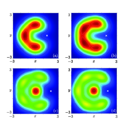
Figure 4: Density plot of the two-body density $\rho_{2}({\bf r},{\bf r}^{\prime})$ (arbitrary units, topographic color-scale: red high and blue low values) for the dot GS with (a) $N=4$; (b) $N=5$; (c) $N=6$; (d) $N=7$ and $\lambda=2.8$. The coordinate ${\bf r}^{\prime}$ of the probe electron is chosen on the external ridge of $\rho_{1}(r)$ and is marked with a white cross in each panel. See text for other physical parameters.

This is confirmed by figure 4, which shows a density plot of $\rho_{2}(\mathbf{r},\mathbf{r}^{\prime})$ for the dot GSs as a function of $\mathbf{r}$ in the $(x,y)$ plane. The white cross denotes the position of $\mathbf{r}^{\prime}$, which is the same as in figure 3. Around $\mathbf{r}^{\prime}$, the presence of the Fermi hole is clear. Strong radial and angular correlations are observed, confirming the structures for $N=4$ (square), $N=5$ (pentagon), $N=6$ (centered pentagon) and $N=7$ (centered hexagon).

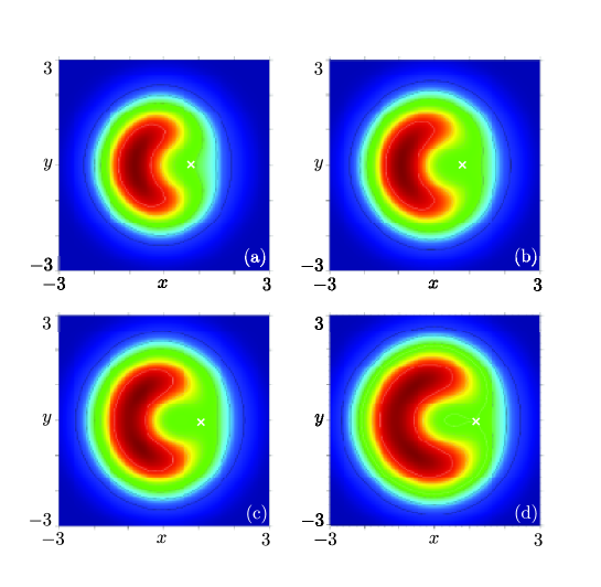
Figure 5: Same as in figure 4 but with $\lambda=1.2$ in all panels.

For comparison, density plots for $\lambda=1.2$ are shown in figure 5. For such a smaller interaction, radial and angular correlations beyond the Fermi hole are undetectable. The situation is more reminiscent of a liquid-like behaviour.
Even though the discussion has been focused on the dot ground state, also the WFs for the excited states behave in a similar manner.
The above results confirm that PHF is able to capture at the qualitative level all the relevant correlations of the dot WFs and to produce Wigner molecular states. In this respect, we note that the onset in $\lambda$ for the development of strong radial and angular correlations in the WFs predicted by the PHF method seems to be smaller than the one found with other techniques. As an example, for $N=6$, both exact diagonalization [56] and density functional [12] calculations predict the localization of one electron in the dot center for $\lambda\approx 8$ while from the PHF calculations one would obtain $\lambda\approx 2$. A similar tendency to underestimate the crossover in $\lambda$ for the transition between different dot GSs has already been observed in earlier studies of PHF [22]. Since the qualitative changes of the dot WF are correctly captured by PHF, we expect that the transport results described below will be at least qualitatively correct.

3.2 Transport properties

In this section we will show how modifications of the WF, occurring in the transition from a liquid to a molecular character, can be detected in the transport properties. In the rest of the paper, we assume symmetric tunnelling barriers, with $\Gamma^{(\mathrm{E})}=\Gamma^{(\mathrm{C})}=\Gamma_{0}$ in (9). Typical values for $\Gamma_{0}$ are of the order of some MHz.

3.2.1 Linear transport

We start considering the linear regime ($V\to 0$), which provides information on the dot ground states.

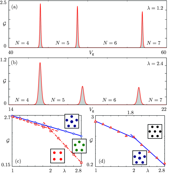
Figure 6: (a) Plot of the linear conductance $\mathcal{G}$ as a function of $V_{\mathrm{g}}$ (units mV) for $T=500$ mK and $\lambda=1.2$. (b) Same as in (a) but for $\lambda=2.4$. (c) Plot of the conductance maxima (log scale) as a function of the interaction strength $\lambda$ for the transition $4\leftrightarrow 5$ (circles) and $5\leftrightarrow 6$ (squares). Lines are a guide for the eye. (d) Same as in (c) but for the transition $6\leftrightarrow 7$. The insets in panels (c,d) represent the structure of the dot GS WF in the strongly correlated regime. Conductance unit $\mathcal{G}_{0}=1.6\cdot 10^{-7}\Gamma_{0}$ s/G$\Omega$

.

A plot of the linear conductance ${\mathcal{G}}$ as a function of $V_{\mathrm{g}}$, calculated solving numerically (11) in the stationary regime is shown in figure 6(a). It has been calculated for $\lambda=1.2$. The conductance exhibits the well known Coulomb oscillations: conductance peaks are separated by regions where the dot is in the Coulomb blockade regime and transport is forbidden [1, 75]. Peaks occur when the chemical potential of the dot is aligned with the electrochemical potential of the leads $\mu_{\mathrm{D}}=\mu_{0}$, which is satisfied for a given transition $N\leftrightarrow N+1$ by suitably tuning $V_{\mathrm{g}}$. Since $\mu_{0}$ simply induces a constant shift of the position of the linear conductance peaks in $V_{\mathrm{g}}$, we assume $\mu_{0}=0$. Turning to stronger interactions $\lambda=2.4$, figure 6(b), the linear conductance decreases. The observed suppression of $\mathcal{G}$ as $\lambda$ is increased can be interpreted as due to the increased difficulty to tunnel into (or out from) an electronic system with strong Coulomb repulsion. However, the conductance peaks for the transition $5\leftrightarrow 6$ and $6\leftrightarrow 7$ have been suppressed much more than that corresponding to $4\leftrightarrow 5$.

In order to investigate this behaviour more systematically, the heights of the conductance peaks are shown in logarithmic scale as a function of $\lambda$ in figure 6(c,d). For the transition $4\leftrightarrow 5$ (circles), a single slope is observed, signalling an exponential suppression of the conductance as $\lambda$ increases. On the other hand, for $5\leftrightarrow 6$ (squares) a bimodal behaviour occurs, with a slope for $\lambda\leq 2$ that is very similar to the one found for $4\leftrightarrow 5$. A steeper slope is found for $\lambda>2$. The conductance peak for the transition $6\leftrightarrow 7$, see figure 6(d), shows a behaviour similar to $5\leftrightarrow 6$: a smaller slope for $\lambda\leq 1.6$ and a steeper one for $\lambda\geq 2$.

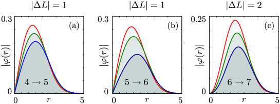
Figure 7: Radial behaviour of the modulus of the QPWF $|\varphi(r)|$ – see (14) – for $\lambda=1.2$ (red), $\lambda=1.8$ (green) and $\lambda=2.4$ (blue) and different transitions between dot GSs: (a) $4\leftrightarrow 5$; (b) $5\leftrightarrow 6$; (c) $6\leftrightarrow 7$. At the top of the panels, $|\Delta L|$ for the given transition is quoted, see table 1.

In order to interpret these behaviours we can deduce more precise information about the tunnelling of electrons from the QPWF, see (14). Figure 7 shows its modulus $|\varphi(r)|$ for the transition between dot GSs $N\to N+1$ with $N=4$ (a), $N=5$ (b) and $N=6$ (c) and increasing values of $\lambda$. Since all these transitions have $|\Delta L|\neq 0$ (see table 1), the WF exhibits an off-center maximum and is small around the origin, hence tunnelling is strongly suppressed in the center while it is enhanced at the edge of the dot. The above transport results are now explained by considering both the shape of the QPWF and the structure of the WF of the dot GS for each $N$, discussed in Sec. 3.1.
On the one hand, by comparing the WFs for two subsequent dot GSs one can estimate where the tunnelling electron should enter in order to provide an optimal matching between the dot states and obtain a good transmission through the dot. On the other hand, the most likely position of the tunnelling electron is essentially dictated by $|\Delta L|$, as the QPWF shows. As a result, a higher conductance is obtained in situations where the QPWF is peaked so as to provide a maximal overlap of the dot WFs. With these considerations, let us now reexamine figure 6(c,d).
For the transition $4\leftrightarrow 5$, as $\lambda$ increases, the dot WFs build up radial and subsequently angular correlations, ending up eventually in a molecular state with a square ($N=4$) or pentagon ($N=5$) symmetry with always a ring-like structure. As such, maximum overlap is achieved when the tunnelling electron jumps to the edge of the dot. This is the case, in agreement with the results of the QPWF, as confirmed by figure 7(a).
The transition $5\leftrightarrow 6$ displays a more interesting double-slope feature. For small $\lambda$, both the dot GS WFs for $N=5$ and $N=6$ display weak correlations and have a ring-like structure. Similar to the case discussed above the tunnelling electron, entering at the edge of the dot, provides an optimal overlap of the dot WFs. Therefore, a slope similar to the one observed for $4\leftrightarrow 5$ is obtained for small $\lambda$. On the other hand, for $\lambda\gtrsim 2$ one electron is shifted towards the center of the dot. Eventually, the WF for $N=6$ acquires the shape of a centered pentagon, see the inset in figure 6(c). The optimal overlap would be achieved with the tunnelling electron jumping to the center of the dot. This however is not allowed for dynamical reasons, as shown by the QPWF in figure 7(b): the tunnelling electron needs to enter into the dot edge. Therefore, an additional suppression of the conductance occurs, which is detected in the sharp change of slope of $\mathcal{G}$ shown in figure 6(c).
In the case of $6\leftrightarrow 7$, for $\lambda<1.8$ correlations in both the WFs are weak and the latter exhibit a ring-like shape as in all the low $\lambda$ regimes already discussed. For $\lambda\approx 1.8$, the GS with $N=7$ begins to shift one electron towards the center of the dot, while the GS of $N=6$ remains annular. Since the QPWF is peaked at the edge of the dot, this corresponds to a slight, yet noticeable, suppression of $\mathcal{G}$ visible in figure 6(d) for $\lambda=1.8$. For $\lambda\geq 2$, also the GS for $N=6$ has one electron in the center of the dot. The optimum overlap is again achieved for tunnelling at the dot edge and therefore one could expect a return of a power law similar to the one observed for $\lambda\leq 1.6$. On the contrary, one observes a steeper slope. In order to explain this phenomenon we need to consider in detail the spin structure of the dot GSs.

We consider here the two states $|N,L,S,S_{z}\rangle=|6,0,0,0\rangle$ and $|7,2,1/2,1/2\rangle$.

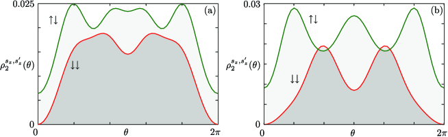
Figure 8: Angular dependence of the spin-resolved two-body density functions $\rho_{2}^{s_{z},s_{z}^{\prime}}(\theta)=\rho_{2}^{s_{z},s_{z}^{\prime}}(r_{0}(N,\lambda),\theta,r_{0}(N,\lambda),0)$ (units: $\ell_{0}^{-4}$) with $s_{z}^{\prime}=-1/2$ and $s_{z}=-1/2$ (red line) or $s_{z}=+1/2$ (green line) for the dot states (a) $|6,0,0,0\rangle$; (b) $|7,2,1/2,1/2\rangle$. Here, $\lambda=2.4$.

Figure 8 shows the spin-resolved two body correlation function $\rho_{2}^{s_{z},s_{z}^{\prime}}(\mathbf{r},\mathbf{r}^{\prime})$ in (19), calculated along the outer ring of the quantum dot GSs for $N=6,7$ and a representative value $\lambda=2.4$. One electron with spin down is assumed to lie at $r^{\prime}=r_{0}(N,\lambda)$ and $\theta^{\prime}=0$. Starting with $N=6$, panel (a), one can see that the probability of finding another spin-down electron ($\rho_{2}^{\downarrow,\downarrow}(\theta)$) is peaked around $\theta\approx 4\pi/5$ and $\theta\approx 6\pi/5$, while the one for an electron with spin up ($\rho_{2}^{\uparrow,\downarrow}(\theta)$) is highest at $\theta=2\pi/5$ and $\theta=8\pi/5$, although two relative maxima for this probability are observed also for $\theta=4\pi/5$ and $\theta=6\pi/5$. For $N=7$ one finds that the probability of finding another spin-down electron ($\rho_{2}^{\downarrow,\downarrow}(\theta)$) is largest at $\theta=2\pi/3$ and $\theta=4\pi/3$, while spin-up electrons are maximally likely at $\theta=\pi/3,\pi,5\pi/3$.

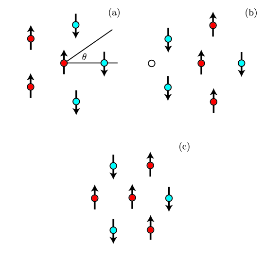
Figure 9: The possible spin pattens, most relevant for linear transport, contributing to the GS WF for $\lambda=2.4$ and (a,b) $N=6$; (c) $N=7$. The probe electron lies at $\theta=0$ and the white dot denotes the preferred site for tunnelling.

In the Wigner molecule regime, only a few different spin configurations may contribute to the dot WF. In the case of $N=6$, once the spin direction for the electron at the center of the dot is chosen, only two possible spin arrangements are possible for the pentagon at the edge. These are shown in Figs. 9(a,b) for the case of a spin up in the dot center. Since the WF for $N=6$ is a spin singlet, also the two other configurations, obtained flipping all spins in panels (a) and (b) are possible (not shown). Since the correlation function in figure 8(a) for parallel spin-down electrons is more peaked around $\theta=4\pi/5$ and $\theta=6\pi/5$, one can anticipate that the configuration represented in panel (b) contributes more than the one in panel (a). Also for $N=7$ several spin configurations for the dot edge exist, once the spin in the center of the dot has been fixed. However, the clear peak structure of figure 8(b) strongly suggests a well-defined texture of alternating spins in the outer ring of the molecule with a corresponding spin-up electron in the center of the dot, consistent with $S_{z}=1/2$. Therefore, we can infer that the dot WF for $N=7$ has the spin structure shown in figure 8(c). Note that the discussion for the other states of the multiplet for $N=7$ is identical, provided that one flips all spins for the states with $S_{z}=-1/2$.
Let us go back to the transport properties of the dot. Among all the possible spin configurations for $N=6$, the ones with a spin down at the dot center, obtained by flipping the spins of those shown in figure 9(a,b), provide a very poor overlap with the state with $N=7$ and therefore can be neglected. The configuration shown in figure 9(a) also provides a negligible overlap: there is no position around the edge for the tunnelling electron so that the final state has the same spin pattern shown in figure 9(c). Concerning the situation shown in Fig 9(b), the tunnelling electron can only jump in the proximity of $\theta=\pi$ (white dot in the figure) since all other positions would lead to a wrong spin pattern on the edge. This results in a suppression of the tunnelling amplitude as compared to the case of small $\lambda<1.8$, when the tunnelling electron is free to delocalize around the ring due to the negligible correlations of the dot WF.
It is important to note that the situation described before does not occur either for $4\leftrightarrow 5$, whose conductance is featureless, or for $5\leftrightarrow 6$ whose change of slope is mainly related to the localization of one electron in the center of the dot.

From the above discussions one can conclude that the transition towards the Wigner molecule, accompanied by qualitative rearrangements of the charge or spin textures of the dot WF, may be detectable in the linear transport properties. This seems particularly relevant when transport involves states with higher numbers of electrons and intricate spin patterns, such as $N=6,7$, due to the complex internal structure. Simpler configurations such as the ones for the transition $4\leftrightarrow 5$ discussed above may not cause any signature in transport. It is worth to notice that the spin effects discussed above are subtler than the more common type-II spin blockade [73, 74]. In the latter, the current flow is blocked due to the impossibility to fulfil total spin conservation by tunneling events. In the Wigner molecule regime, on the other hand, even if spin conservation is satisfied an additional suppression of the current as $\lambda$ increases occurs, due to the peculiar internal spin structure of the dot WFs.

3.2.2 Nonlinear transport

In the nonlinear regime, transport also triggers the population of excited states of the quantum dot. In this section we discuss one particular case, to show signatures of the transition towards the Wigner molecule. To be specific, we will concentrate on the regime where only states with $N=5,6$ electrons in the dot are involved. Furthermore, we assume strong relaxation: $W\gg\Gamma_{0}$, see (12).

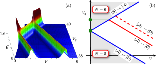
Figure 10: (a) Nonlinear conductance $\mathcal{G}$ (units $\mathcal{G}_{0}$ same as in figure 6) as a function of applied voltage $V$ (units mV) and gate voltage $V_{\mathrm{g}}$ (units mV) for $\lambda=1.4$, $T=750$ mK and $W=50\Gamma_{0}$. (b) Scheme of the transitions involving the ground states for $N=5,6$ and the lowest lying excited states for $N=6$. The dashed line represents a spin-blockaded transition not visible in the sequential regime.

Table 2: States and corresponding quantum numbers involved in transport dynamics for the range of $V$ and $V_{\mathrm{g}}$ considered in figure 10.

• State	N	L	S	$S_{z}$
  $|{\mathcal{A}}\rangle$	5	$\pm 1$	1/2	$\pm 1/2$
  $|{\mathcal{B}}\rangle$	6	0	0	0
  $|{\mathcal{C}}\rangle$	6	$\pm 1$	1	0,$\pm 1$
  $|{\mathcal{D}}\rangle$	6	0	2	0,$\pm 1$,$\pm 2$

The numerically evaluated $\mathcal{G}$ as a function of $V$ and $V_{\mathrm{g}}$ is shown in figure 10(a) for $\lambda=1.4$. It exhibits conductance lines corresponding to transitions between the dot GSs or between GS and lowest-lying excited states. The scheme of the expected lines is shown in figure 10(b) for the voltages region considered here. The transitions corresponding to each line are shown, with their quantum numbers given in table 2. The blue lines represent transitions between the dot GSs for $N=5$ ($|{\mathcal{A}}\rangle$) and $N=6$ ($|{\mathcal{B}}\rangle$). The red lines represent channels involving the GS of $N=5$ ($|{\mathcal{A}\rangle}$) and one of the first two excited multiplets of $N=6$: the lowest one is denoted as $|{\mathcal{C}}\rangle$ while the next-to-lowest is $|{\mathcal{D}}\rangle$. Since calculations are performed for temperatures smaller than the average level spacing between the dot multiplets, in the strong relaxation regime transitions among the excited states of the dot cannot occur. Each of these transition lines corresponds to the opening of the specific transport channel involving an excited state of the dot with $N=6$. Note that transitions involving excited states for $N=5$ are not present in the considered range of $V$ and $V_{\mathrm{g}}$, since they lie at higher energies. A comparison between the scheme of figure 10(b) and the calculated conductance, figure 10(a) shows that only the first transition line (red solid), corresponding to $|{\mathcal{A}}\rangle\to|{\mathcal{C}}\rangle$ is observed, while the one corresponding to the second excited multiplet of $N=6$ (red dashed) is absent. By inspecting table 2, one notes that the transition $|{\mathcal{A}}\rangle\to|{\mathcal{D}}\rangle$ involves $|\Delta S|>1/2$ and therefore is forbidden [73, 74], leading to a vanishing conductance.

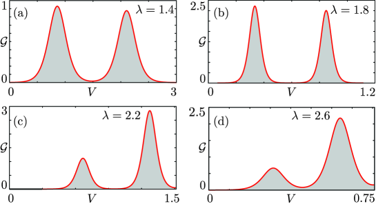
Figure 11: Nonlinear conductance as a function of the applied voltage $V$ (units mV) near the transition $5\leftrightarrow 6$ for (a) $\lambda=1.4$, $V_{\mathrm{g}}=39.3$ mV, $T=750$ mK; (b) $\lambda=1.8$, $V_{\mathrm{g}}=27.3$ mV, $T=150$ mK; (c) $\lambda=2.2$, $V_{\mathrm{g}}=20.2$ mV, $T=150$ mK; (d) $\lambda=2.6$, $V_{\mathrm{g}}=15.9$ mV, $T=100$ mK. In all plots, $W=50\Gamma_{0}$ and the conductance unit $\mathcal{G}_{0}$ is the same as in figure 6.

Figure 11 shows plots of $\mathcal{G}$ as a function of the applied voltage for different values of $\lambda$. In all panels, the value of $V_{\mathrm{g}}$ has been chosen to lie between the green square and the green dot in figure 10(b). The peak at lower $V$ in Figs. 11(a–d) corresponds to the GS to GS transition $|{\mathcal{A}}\rangle\to|{\mathcal{B}}\rangle$, while the second one to the transition $|{\mathcal{A}}\rangle\to|{\mathcal{C}}\rangle$. As is visible from the voltage ranges of the plots, the dot level spacing (corresponding to the distance between the nonlinear conductance peaks) gets narrower as $\lambda$ is increased. In order to be able to resolve both conductance peaks, calculations for higher $\lambda$ have been performed at lower temperatures than those at smaller $\lambda$.
Comparing the panels (a) and (b) for $\lambda<2$ with panels at $\lambda>2$ (c) and (d), a qualitative difference in the behaviour is easily observed: for weaker interaction strengths, the first peak is always higher than the second one, while for $\lambda>2$ the situation reverses drastically.
Such a behaviour cannot be attributed to the difference in temperature between different calculations. Indeed, calculations for $\lambda=1.4$ and $\lambda=1.8$ performed at lower temperatures display narrower conductance peaks but still with almost equal height. Increasing $T$ for $\lambda=2.2$ and $\lambda=2.6$ always suppresses the conductance for the GS to GS peak with respect to the transition towards the excited state in all the temperature range in which the two peaks are resolved.

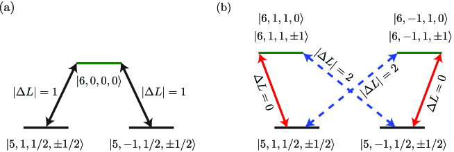
Figure 12: (a) Scheme of the transitions involved in the first conductance peak shown in figure 11. (b) Same as in (a) but for the second conductance peak.

The behaviour of the nonlinear conductance can be related to qualitative changes in the WFs of the excited states for $N=6$. Figure 12 shows the states involved in the transport dynamics of the two conductance peaks discussed above. The height of each peak is determined by the available transport channels and by the transition rates connecting the dot states. As the interaction strength is increased the first conductance peak, involving only transitions between GSs – see figure 12(a) – behaves exactly as the linear conductance peak discussed in Sec. 3.2.1. The height of the second peak is on the other hand determined by two families of transport channels connecting the GS with $N=5$ to the excited multiplet of $N=6$: as shown in figure 12(b), channels with either $\Delta L=0$ or $|\Delta L|=2$ are possible. The corresponding transition amplitudes are shown in figure 13(a) as a function of $\lambda$. Transition rates are proportional to these amplitudes, see (9). One can see that for $\lambda<2$ the transition channel with $\Delta L=0$ is strongly suppressed, while the one with $|\Delta L|=2$ is larger and decaying with $\lambda$. For $\lambda>2$, a sudden decrease of the transition amplitude for the channel with $|\Delta L|=2$ is found, while the one for the channel with $\Delta L=0$ jumps to a very large value.

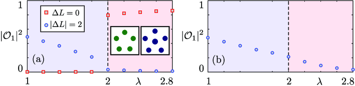
Figure 13: (a) Squared modulus of the transition amplitude $|\mathcal{O}_{1}|^{2}$ – see (10) – for the processes $|5,\pm 1,1/2,\pm 1/2\rangle\to|6,\mp 1,1,\pm 1\rangle$ with $|\Delta L|=2$ (circles) and $|5,\pm 1,1/2,\pm 1/2\rangle\to|6,\pm 1,1,\pm 1\rangle$ with $\Delta L=0$ (squares) shown in figure 12(b). The insets show the character of the dot WF for high values of $\lambda$. (b) Same as in (a) but for the GS to GS transition $|5,\pm 1,1/2,\pm 1/2\rangle\to|6,0,0,0\rangle$ shown in figure 12(a). Amplitudes for transitions involving triplet states with $S_{z}=0$ are proportional to the ones shown here, the proportionality constant being a Clebsch-Gordan factor $1/\sqrt{2}$. Amplitudes for transitions with $|\Delta S_{z}|>1/2$ are zero.

This peculiar behaviour can be again explained using the QPWFs.

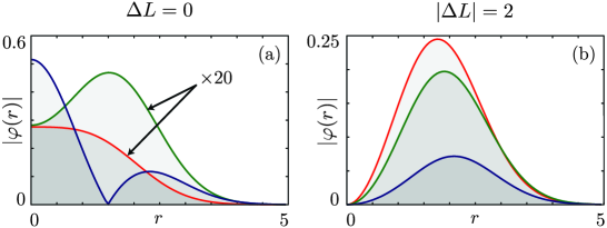
Figure 14: Radial behaviour of the modulus of the QPWF $|\varphi(r)|$ for $\lambda=1.2$ (red) $\lambda=1.8$ (green) and $\lambda=2.4$ (blue) and different processes: (a) $5\leftrightarrow 6$ GS to first excited with $\Delta L=0$, i.e. $|5,\pm 1,1/2,\pm 1/2\rangle\leftrightarrow|6,\pm 1,1,\pm 1\rangle$; (b) $5\leftrightarrow 6$ GS to first excited with $|\Delta L|=2$, i.e. $|5,\pm 1,1/2,\pm 1/2\rangle\leftrightarrow|6,\mp 1,1,\pm 1\rangle$. Note that in (a), the red and green curves for $\lambda=1.2$ and $\lambda=1.8$ have been magnified by a factor 20.

Figure 14 shows the QPWF for the transition with $\Delta L=0$ (panel a) and for the one with $\Delta L=2$ (panel b). When $\lambda<2$, the case of $\Delta L=0$ has nonzero amplitude near the center of the dot and consequently a very small overlap between the configurations for $N=5$ and $N=6$ which have a ring-like character. This results in a very small transition amplitude. On the other hand, the case of $|\Delta L|=2$ has a large QPWF near the edge of the dot and therefore provides a much better overlap between the dot configurations. The situation reverses dramatically for $\lambda>2$: the developing radial correlations induce a qualitative change in the dot WF for $N=6$ and one electron moves near the center of the dot, in analogy to the case of the GS. In this case, a much better overlap occurs for $\Delta L=0$, since the extra electron preferably sits in the center of the dot, see the right insets in figure 13(a). The transition with $|\Delta L|=2$ is strongly suppressed since the corresponding QPWF is $\propto r^{2}$ and thus negligible near the dot center.
Therefore, for $\lambda<2$ transport through the excited state occurs essentially via the channel with $|\Delta L|=2$, whose amplitude is similar to the one for the GS to GS transition, see figure 13(b). This explains why, for $\lambda<2$, the two conductance peaks in figure 11(a,b) have almost equal height. For $\lambda>2$ the channel with $\Delta L=0$ clearly dominates, due the peculiar rearrangement of the dot WF for $N=6$ moving towards the Wigner molecule. The amplitude for this channel is larger than the one for the GS to GS transition and therefore the conductance peak for the transition involving the excited state is higher than the one for the GS to GS transition as shown in figure 11(c,d).

4 Conclusions

In this paper we have investigated correlation effects in a quantum dot via linear and nonlinear transport, employing the PHF technique. For increasing interaction strength, the ground and excited dot states have been analyzed for $4\leq N\leq 7$. As the strength of the Coulomb interactions increases, the dot WFs build up radial and angular correlations, smoothly crossing over from a liquid-like regime to Wigner molecular states. Most strikingly, we have demonstrated that signatures of such a crossover may appear both in the linear and in the nonlinear transport properties. These signatures have been interpreted with the systematic study of both two-body correlation functions and QPWFs.
In the linear regime, we have observed an exponential suppression of the conductance as the transition towards the Wigner molecule takes place. In cases when the latter is accompanied by strong qualitative rearrangements of the dot WFs, strong mismatches of the dot WFs involved in the transport process may occur. This leads to a stronger suppression of the conductance, as observed for the case $5\leftrightarrow 6$. A mismatch of the dot WFs due to the emergence of particular spin structure of the dot states may also occur, as exemplified by the case of $6\leftrightarrow 7$. Also this fact leads to an increased suppression of the linear conductance.
In the nonlinear regime, the conductance may even be enhanced by the formation of a Wigner molecule within the dot, as shown by the study of the transport dynamics of the lowest-lying excited states for $N=6$.
The effects described above are due to the qualitative rearrangements of the charge or spin patterns of the dot states, occurring during the transition towards the Wigner molecule regime. As a possible extension of this investigation, it would be interesting to devise a method to investigate the internal spin structure of the Wigner molecule, e.g. by analyzing the effects of spin-dependent tunnel barriers. Effects due to Wigner molecules should have a profound impact in coherent regimes and could lead to strong signatures detected by analyzing e.g. the cotunnelling regime. Finally, it would be interesting to consider the effects of applied magnetic fields, which are known to strongly modify the properties of Wigner molecules.
We expect that results similar to the ones shown in this paper hold also for planar quantum dots and that they could be in principle observed experimentally.

Appendix A Tunnelling Hamiltonian

In this appendix we derive $\hat{H}_{\mathrm{t}}$ for a quantum dot connected to two external emitter or collector leads via tunnelling barriers located around $z=z_{\alpha}$ ($\alpha=\mathrm{E,C}$), see figure 1. Our starting point is the Bardeen tunnelling Hamiltonian [83]

$$\!\!\!\!\!\!\!\!\!\!\!\!\hat{H}_{\mathrm{t}}=\frac{i}{2m^{*}}\sum_{\alpha=\mathrm{E,C}}\int{\mathrm{d}}\mathbf{R}\ {\mathrm{d}}z\ \delta(z-z_{\alpha})\left[\hat{\Psi}^{\dagger}(\mathbf{R},z)\frac{\partial\hat{\Psi}(\mathbf{R},z)}{\partial z}-\mathrm{h.c.}\right]\,.$$ (21)

Here, ${\mathbf{R}}=(x,y)$ and $z_{\alpha}$ is a point within the tunnelling barrier between the lead $\alpha$ and the dot. Furthermore, $\hat{\Psi}(\mathbf{R},z)$ is the system field operator expanded into emitter, dot and collector contributions as $\hat{\Psi}(\mathbf{R},z)=\hat{\Psi}_{\mathrm{D}}(\mathbf{R},z)+\sum_{\alpha=\mathrm{E,C}}\hat{\Psi}_{\alpha}(\mathbf{R},z)$ with

$$\hat{\Psi}_{\alpha}(\mathbf{R},z) = \sum_{\xi_{\alpha}}\Phi_{\xi_{\alpha}}^{(\alpha)}(\mathbf{R},z)\hat{c}_{\alpha,\xi_{\alpha}}$$ (22)

$$\hat{\Psi}_{\mathrm{D}}(\mathbf{R},z) = \sum_{\eta}\Phi_{\eta}^{(\mathrm{D})}(\mathbf{R},z)\hat{d}_{\eta}\,.$$ (23)

Here, $\Phi_{\xi_{\alpha}}^{(\alpha)}(\mathbf{R},z)$ and $\Phi_{\eta}^{(\mathrm{D})}(\mathbf{R},z)$ are a set of single particle eigenfunctions for leads and dot, respectively. Note that these sets may be complete but leads and dot states need not be orthogonal. In the following, we assume that the longitudinal ($z$) and transverse ($x,y$) motions are decoupled, which allows the factorizations of the single particle WFs. Furthermore, we will concentrate on a system with cylindrical symmetry. For the leads one has $\Phi_{\xi_{\alpha}}^{(\alpha)}(\mathbf{R},z)=\phi_{\nu_{\alpha}}(\mathbf{R})\chi_{k_{\alpha}}(z)$ where $k_{\alpha}$ is the momentum along the $z$ direction and $\nu_{\alpha}$ is a set of quantum numbers describing the transverse motion. For the quantum dot we choose $\Phi_{\eta}^{(\mathrm{D})}(\mathbf{R},z)=\phi_{\eta}(\mathbf{R})\chi_{\mathrm{D}}(z)$, where $\eta=\{n_{\eta}^{({\mathrm{D}})},l_{\eta}^{({\mathrm{D}})},s_{z\eta}^{({\mathrm{D}})}\}$ collectively denotes the FD quantum numbers. Choosing the basis of FD states is not restrictive: as shown in C, every orthonormal and complete basis for the single particle states of the dot is equivalent. We assume a sufficiently tight confinement in the $z$ direction so that longitudinal motion of electrons in the dot is effectively frozen into the lowest subband with WF $\chi_{\mathrm{D}}(z)$. The longitudinal dot WF $\chi_{\mathrm{D}}(z)$ is evanescent within both tunnelling barriers. For the leads, $\chi_{k_{\mathrm{E}}}(z)$ ($\chi_{k_{\mathrm{C}}}(z)$) is evanescent under the tunnelling barrier near the emitter (collector) and essentially zero near the collector (emitter). Substituting the explicit expressions of the field operators into (21) and taking into account the form of the single particle WFs one obtains $\hat{H}_{\mathrm{t}}=\hat{H}_{\mathrm{t}}^{(0)}+\hat{H}_{\mathrm{t}}^{(1)}$ with

$$\hat{H}_{\mathrm{t}}^{(0)} = \sum_{\alpha=\mathrm{E,C}}\sum_{\xi_{\alpha},\xi^{\prime}_{\alpha}}\Delta_{\xi_{\alpha},\xi^{\prime}_{\alpha}}^{(\alpha)}\hat{c}^{\dagger}_{\alpha,\xi_{\alpha}}\hat{c}_{\alpha,\xi^{\prime}_{\alpha}}+\Delta^{(\mathrm{D})}\sum_{\eta}\hat{d}^{\dagger}_{\eta}\hat{d}_{\eta}$$ (24)

$$\hat{H}_{\mathrm{t}}^{(1)} = \sum_{\alpha=\mathrm{E,C}}\sum_{\xi_{\alpha},\eta}\tau_{\xi_{\alpha},\eta}^{(\alpha)}\hat{c}^{\dagger}_{\alpha,\xi_{\alpha}}\hat{d}_{\eta}+\mathrm{h.c.}\,,$$ (25)

where

$$\Delta_{\xi_{\alpha},\xi^{\prime}_{\alpha}}^{(\alpha)} = \frac{i}{2m^{*}}\delta_{\nu_{\alpha},\nu^{\prime}_{\alpha}}\left[\chi^{*}_{k_{\alpha}}(z_{\alpha})\left.\frac{\partial\chi_{k^{\prime}_{\alpha}}(z)}{\partial z}\right|_{z_{\alpha}}-\chi_{k^{\prime}_{\alpha}}(z_{\alpha})\left.\frac{\partial\chi_{k^{\prime}_{\alpha}}^{*}(z)}{\partial z}\right|_{z_{\alpha}}\right]\,,$$

$$\Delta^{(\mathrm{D})} = \frac{i}{2m^{*}}\sum_{\alpha=\mathrm{E,C}}\left[\chi^{*}_{\mathrm{D}}(z_{\alpha})\left.\frac{\partial\chi_{\mathrm{D}}(z)}{\partial z}\right|_{z_{\alpha}}-\chi_{\mathrm{D}}(z_{\alpha})\left.\frac{\partial\chi_{\mathrm{D}}^{*}(z)}{\partial z}\right|_{z_{\alpha}}\right]\,,$$

$$\tau_{\xi_{\alpha},\eta}^{(\alpha)} = \frac{i}{2m^{*}}\left[\chi^{*}_{k_{\alpha}}(z_{\alpha})\left.\frac{\partial\chi_{\mathrm{D}}(z)}{\partial z}\right|_{z_{\alpha}}-\chi_{\mathrm{D}}(z_{\alpha})\left.\frac{\partial\chi_{k_{\alpha}}^{*}(z)}{\partial z}\right|_{z_{\alpha}}\right]\cdot$$ (26)

$$\cdot\int{\mathrm{d}}\mathbf{R}\ \phi_{\nu_{\alpha}}^{*}(\mathbf{R})\phi_{\eta}(\mathbf{R})\,.$$

The first term in $\hat{H}_{\mathrm{t}}^{(0)}$ produces a weak, one-body scattering within the leads, while the second term gives rise to a small uniform shift of the dot energy levels. Both effects can be safely neglected. The relevant term is $\hat{H}_{\mathrm{t}}^{(1)}$, which produces scattering of electrons between the leads and the dot. For a pillar quantum dot, assuming harmonic confinement of electrons in the emitter and collector, with frequency $\omega_{\alpha}$, the WFs $\phi_{\nu_{\alpha}}(\mathbf{R})$ are FD states. We consider the case $\omega_{\alpha}\approx\omega$. Equation (26) yields essentially

$$\tau_{\xi_{\alpha},\eta}=t_{k_{\alpha}}^{(\alpha)}\delta_{\nu_{\alpha},\eta}\approx t^{(\alpha)}\delta_{\nu_{\alpha},\eta}$$ (27)

where in the last equality we have neglected the weak dependence of the tunneling matrix element on $k_{\alpha}$. Finally, the tunnelling Hamiltonian assumes the form

$$\hat{H}_{\mathrm{t}}=\sum_{\alpha}t^{(\alpha)}\sum_{\xi_{\alpha},\eta}\hat{c}^{\dagger}_{\alpha,\xi_{\alpha}}\hat{d}_{\eta}+\mathrm{h.c.}\,.$$ (28)

Appendix B Tunnelling rates

In the sequential regime, tunnelling rates between initial $|\mathcal{I}\rangle$ and final $|\mathcal{F}\rangle$ states of the system are obtained via the Fermi’s golden rule [84]

$$\Gamma_{{\mathcal{I}}\to{\mathcal{F}}}=2\pi\left|\langle\mathcal{F}|\hat{H}_{\mathrm{t}}|\mathcal{I}\rangle\right|^{2}\delta(E_{\mathcal{F}}-E_{\mathcal{I}})\,,$$ (29)

where $E_{\mathcal{I}}$ ($E_{\mathcal{F}}$) is the total energy of the system in the initial (final) state and

$$|\mathcal{I}\rangle=|\mathcal{I}_{\mathrm{E}}\rangle\otimes|\mathcal{I}_{\mathrm{C}}\rangle\otimes|\mathcal{I}_{\mathrm{D}}\rangle\quad;\quad|\mathcal{F}\rangle=|\mathcal{F}_{\mathrm{E}}\rangle\otimes|\mathcal{F}_{\mathrm{C}}\rangle\otimes|\mathcal{F}_{\mathrm{D}}\rangle\,,$$

where $|\mathcal{I}_{\alpha}\rangle$ ( $|\mathcal{F}_{\alpha}\rangle$) is the initial (final) state for lead $\alpha$ while $|\mathcal{I}_{\mathcal{D}}\rangle$ ($|\mathcal{F}_{\mathcal{D}}\rangle$) is the dot initial (final) state, with electron number $N_{\mathcal{I}_{\mathrm{D}}}$ ($N_{\mathcal{F}_{\mathrm{D}}}$) and energy $E_{{\mathcal{I}}_{\mathrm{D}}}$ ($E_{{\mathcal{F}}_{\mathrm{D}}}$). Note that dot states can be either ground or excited. In order to have a nonvanishing contribution in the sequential regime, $|N_{{\mathcal{F}}_{\mathrm{D}}}-N_{{\mathcal{I}}_{\mathrm{D}}}|=1$ must hold. This implies that (29) is diagonal in the barrier index $\alpha$ and that sequential tunnelling events through the barriers are independent. The tunnelling rate has the general structure

$$\Gamma_{\mathcal{I}\to\mathcal{F}}=\sum_{\alpha=\mathrm{E,C}}\sum_{p=\pm 1}\Gamma_{\mathcal{I}\to\mathcal{F}}^{(\alpha),p}\,,$$

where the contribution with $p=+1$ ($p=-1$) represents tunnelling into (out from) the dot via lead $\alpha$.
Since we are interested into the dot dynamics only, we perform a thermal average over $|{\mathcal{I}}_{\alpha}\rangle$ and a summation over $|{\mathcal{F}}_{\alpha}\rangle$ obtaining transition rates among dot states only

$$\Gamma_{\mathcal{I}_{\mathrm{D}}\to\mathcal{F}_{\mathrm{D}}}=\sum_{\alpha=\mathrm{E,C}}\sum_{p=\pm 1}\Gamma_{\mathcal{I}_{\mathrm{D}}\to\mathcal{F}_{\mathrm{D}}}^{(\alpha),p}\,.$$ (30)

The leads are assumed to be in equilibrium with respect to their electrochemical potentials $\mu_{\alpha}=\mu_{0}+\delta\mu_{\alpha}$, where $\delta\mu_{\alpha}$ is a shift due to the presence of an applied bias voltage $V$. In the case of a pillar dot, see (28), one obtains

$$\Gamma_{\mathcal{I}_{\mathrm{D}}\to\mathcal{F}_{\mathrm{D}}}^{(\alpha),p}=\Gamma^{(\alpha)}\left|\mathcal{O}_{p}\right|^{2}f_{p}(\mu_{\mathrm{D}}-\mu_{\alpha})\,,$$ (31)

where $\mathcal{O}_{p}$:

$$\mathcal{O}_{1}=\sum_{\eta}\langle\mathcal{F}_{\mathrm{D}}|\hat{d}_{\eta}^{\dagger}|\mathcal{I}_{\mathrm{D}}\rangle\quad;\quad\mathcal{O}_{-1}=\sum_{\eta}\langle\mathcal{F}_{\mathrm{D}}|\hat{d}_{\eta}|\mathcal{I}_{\mathrm{D}}\rangle\,,$$ (32)

and $f_{p}(E)=pf(E)+(1-p)/2$, with $f(E)=[1+\exp(\beta E)]^{-1}$ the Fermi distribution at inverse temperature $\beta=1/k_{\mathrm{B}}T$ ($k_{\mathrm{B}}$ the Boltzmann constant) and $\mu_{\mathrm{D}}=E_{{\mathcal{F}}_{\mathrm{D}}}-E_{{\mathcal{I}}_{\mathrm{D}}}$.

Appendix C Equivalence of different bases

In this appendix we will show the equivalence of different single particle bases of the dot for the definition of the tunneling Hamiltonian. Consider two orthonormal and complete bases of single particle dot states labeled by $\{\eta\}$ and $\{\mu\}$, with corresponding orbitals $\phi_{\eta}(\mathbf{R})$, $\bar{\phi}_{\mu}(\mathbf{R})$ and Fermi operators $d_{\eta}$, $\bar{d}_{\mu}$ (in this section we omit overhats from the operators to simplify the notation). They are connected by a unitary matrix $M_{\eta\mu}$

$$\phi_{\eta}(\mathbf{R})=\sum_{\mu}M_{\eta\mu}\bar{\phi}_{\mu}(\mathbf{R})\ \ ;\ \ d_{\eta}=\sum_{\mu}M_{\eta\mu}^{\dagger}\bar{d}_{\mu}\,.$$ (33)

The tunneling Hamiltonian, expressed in the basis $\{\mu\}$ reads

$$H_{\mathrm{t}}^{(1)}=\sum_{\alpha=\mathrm{E,C}}\sum_{\xi_{\alpha},\mu}\bar{\tau}_{\xi_{\alpha},\mu}^{(\alpha)}c^{\dagger}_{\alpha,\xi_{\alpha}}\bar{d}_{\mu}+\mathrm{h.c.}\,,$$ (34)

with

$$\bar{\tau}_{\xi_{\alpha},\mu}^{(\alpha)} = \frac{i}{2m^{*}}\left[\chi^{*}_{k_{\alpha}}(z_{\alpha})\left.\frac{\partial\chi_{\mathrm{D}}(z)}{\partial z}\right|_{z_{\alpha}}-\chi_{\mathrm{D}}(z_{\alpha})\left.\frac{\partial\chi_{k_{\alpha}}^{*}(z)}{\partial z}\right|_{z_{\alpha}}\right]\cdot$$ (35)

$$\cdot\int{\mathrm{d}}\mathbf{R}\ \phi_{\nu_{\alpha}}^{*}(\mathbf{R})\bar{\phi}_{\mu}(\mathbf{R})\,,$$

see (26). Inverting (33) for $\bar{d}_{\mu}$ and plugging into (34) one obtains

$$H_{\mathrm{t}}^{(1)}=\sum_{\alpha=\mathrm{E,C}}\sum_{\xi_{\alpha},\eta}\left[\sum_{\mu}M_{\eta\mu}\bar{\tau}_{\xi_{\alpha},\mu}^{(\alpha)}\right]c^{\dagger}_{\alpha,\xi_{\alpha}}d_{\eta}+\mathrm{h.c.}\,.$$ (36)

By virtue of (33), one can easily see that

$$\sum_{\mu}M_{\eta\mu}\bar{\tau}_{\xi_{\alpha},\mu}^{(\alpha)}\equiv\tau_{\xi_{\alpha},\eta}^{(\alpha)}$$ (37)

which shows that (34) is identical to (25). This implies that all results are independent of the choice of the single particle states for the dot.

References

References

- [1] Kouwenhoven L P, Marcus C M, McEuen P L, Tarucha S, Westervelt R M and Wingreen N S 1997 Electron transport in quantum dots (NATO Advanced Studies Institute, Series E: Applied Science) ed. Sohn L L, Kouwenhoven L P and Schön G (Dordrecht: Kluwer) p. 105
- [2] Reimann S M and Manninen M 2002 Rev. Mod. Phys. 74 1283
- [3] Yannouleas C and Landman U 2007 Rep. Prog. Phys. 70 2067
- [4] Delerue C and Lannoo M 2004 Nanostructures: theory and modelling (Berlin: Springer Verlag)
- [5] Taut M 1993 Phys. Rev. A 48 3561
- [6] Zhu J -L, Yu J -Z, Li Z -Q and Kawazoe Y 1996 J. Phys: Condens. Matter 8 7857
- [7] Dineykhan M and Nazmitdinov 1997 Phys. Rev. B 55 13707
- [8] Yannouleas C and Landman U 1999 Phys. Rev. Lett. 82 5325 ; Yannouleas C and Landman U 2000 Phys. Rev. Lett. 85 2220
- [9] Yannouleas C and Landman U 2003 Phys. Rev. B 68 035325
- [10] Reusch B, Häusler W and Grabert H 2001 Phys. Rev. B 63 113313
- [11] Szafran B, Bednarek S, Adamowski J, Tavernier M B, Anisimovas E and Peeters F M 2004 Eur. Phys. J. D 28 373
- [12] Gattobigio M, Capuzzi P, Polini M, Asgari R and Tosi M P 2005 Phys. Rev. B 72 045306
- [13] Koskinen M, Manninen M and Reimann S M 1997Phys. Rev. Lett. 79 1389
- [14] Harju A, Saarikoski H and Räsänen E 2006 Phys. Rev. Lett. 96 126805
- [15] Räsänen E, Könemann J, Haug R J, Puska M J, and Nieminen R M 2004 Phys. Rev. B 70 115308
- [16] Saarikoski H, Tölö E, Harju A and Räsänen E 2008 Phys. Rev. B 78 195321
- [17] Müller H –M and Koonin S E 1996 Phys. Rev. B 54 14532
- [18] Yannouleas C and Landman U 2000 Phys. Rev. B 61 15895
- [19] Yannouleas C and Landman U 2004 Phys. Rev. B 69 113306
- [20] Li Y, Yannouleas C and Landman U 2006 Phys. Rev. B 73 075301
- [21] De Giovannini U, Cavaliere F, Cenni R, Sassetti M and Kramer B 2007 New J. Phys 9 93
- [22] De Giovannini U, Cavaliere F, Cenni R, Sassetti M and Kramer B 2008 Phys. Rev. B 77 035325
- [23] Cavaliere F, De Giovannini U, Cenni R, Sassetti M and Kramer B 2008 Physica E 40 1427
- [24] Serra L, Nazmitdinov R G and Puente A 2003 Phys. Rev. B 68 035341
- [25] Puente A, Serra L and Nazmitdinov R G 2004 Phys. Rev. B 69 125315
- [26] Egger R, Häusler W, Mak C H and Grabert H 1999 Phys. Rev. Lett. 82 3320; Egger R, Häusler W, Mak C H and Grabert H 1999 Phys. Rev. Lett. 83 462
- [27] Ghosal A, Güclü A D, Umrigar C J, Ullmo D and Baranger H U 2006 Nature Physics 2 336
- [28] Ghosal A, Güclü A D, Umrigar C J, Ullmo D and Baranger H U 2007 Phys. Rev. B 76 085341
- [29] Güclü A D, Ghosal A, Umrigar C J and Baranger H U 2008 Phys. Rev. B 77 041301
- [30] Pfannkuche D, Gudmundsson V and Maksym A P 1993 Phys. Rev. B 47 2244
- [31] Imamura H, Aoki H and Maksym P A 1998 Phys. Rev. B 57 R4257
- [32] Yannouleas C and Landman U 2000 Phys. Rev. Lett. 85 1726
- [33] Mikhailov S A 2002 Phys. Rev. B 65 115312
- [34] Mikhailov S A 2002 Phys. Rev. B 66 153313
- [35] Mikhailov S A and Savostianova N A 2002 Phys. Rev. B 66 033307
- [36] Tavernier M B, Anisimovas E, Peeters F M, Szafran B, Adamowski J and Bednarek S 2003 Phys. Rev. B 68 205305
- [37] Tavernier M B, Anisimovas E and Peeters F M 2006 Phys. Rev. B 74 125305
- [38] Anisimovas E,Tavernier M B and Peeters F M 2006 Physica E 40 1621
- [39] Rontani M, Cavazzoni C, Bellucci D and Goldoni G 2006 J. Chem. Phys. 124 124102
- [40] Kouwenhoven L P, Oosterkamp T H, Danoesastro M W S, Eto M, Austing D G, Honda T and Tarucha S 1997 Science 278 1788
- [41] Tarucha S, Austing D G, Honda T, van der Hage R J and Kouwenhoven L P 1996 Phys. Rev. Lett. 77 3613
- [42] Sasaki S, Austing D G and Tarucha S 1998 Physica B 256 157
- [43] Kouwenhoven L P, Austing D G and Tarucha S 2001 Rep. Prog. Phys. 64 701
- [44] Bedanov V M and Peeters F M 1994 Phys. Rev. B 49 2667
- [45] Maksym P A 1996 Phys. Rev. B 53 10871
- [46] Reimann S M, Koskinen M and Manninen M 2000 Phys. Rev. B 62 8108
- [47] Filinov A V, Bonitz M and Lozovik Yu E 2001 Phys. Rev. Lett. 86 3851
- [48] Koskinen M, Manninen M, Mottelson B and Reimann S M 2001 Phys. Rev. B 63 205323
- [49] Saint Jean M, Even C and Guthmann C 2001 Europhys. Lett. 55 45
- [50] Harju A, Siljamäki S and Nieminen R M 2002 Phys. Rev. B 65 075309
- [51] Reusch B and Egger R 2003 Europhys. Lett. 64 84
- [52] Szafran B, Peeters F M, Bednarek S and Adamowski J 2004 Phys. Rev. B 69 125344
- [53] Weiss S and Egger R 2005 Phys. Rev. B 72 245301
- [54] Ludwig P, Balzer K, Filinov A, Stolz H and Bonitz M 2008 New. J. Phys. 10 083031
- [55] Rontani M, Molinari E, Maruccio G, Janson M, Schramm A, Meyer C, Matsui T, Heyn C, Hansen W and Wiesendanger R 2007 J. Appl. Phys. 101 081714
- [56] Rontani M and Molinari E 2005 Phys. Rev. B 71 233106
- [57] Kalliakos S , Rontani M, Pellegrini V, Garcìa C P , Pinczuk A, Goldoni G, Molinari E, Pfeiffer L N and West K W 2008 Nature Physics 4 467
- [58] Zeng L, Geist W, Ruan W Y, Umrigar C J and Chou M Y 2009 Phys. Rev. B 79 235334
- [59] Wigner E P 1934 Phys. Rev. 46 1002
- [60] Giuliani G and Vignale G F 2005 Quantum theory of the electron liquid (Cambridge: Cambridge University Press)
- [61] Jauregui K, Häusler W and Kramer B 1993 Europhys. Lett. 24 581
- [62] Szafran B, Peeters F M, Bednarek S, Chwiej T and Adamowski J 2004 Phys. Rev. B 70 035401
- [63] Xianlong G, Polini M, Asgari R and Tosi M P 2006 Phys. Rev. A 73 033609
- [64] Abedinopur S M, Polini M, Xianlong G and Tosi M P 2007, Phys. Rev. A 75 015602
- [65] Secchi A and Rontani M 2009 Phys. Rev. B 80 0414040
- [66] Garcia C P, Pellegrini V, Pinczuk A, Rontani M, Goldoni G, Molinari E, Dennis B S, Pfeiffer L N and West K W 2005 Phys. Rev. Lett. 95 266806
- [67] Bester G, Reuter D, He L, Zunger A, Kailuweit P, Wieck A D, Zeitler U, Maan J C, Wibbelhoff O and Lorke A 2007 Phys. Rev. B 76 075338
- [68] Kleimann T, Cavaliere F, Sassetti M and Kramer B 2002 Phys. Rev. B 66 165311
- [69] Cavaliere F, Braggio A, Stockburger J T, Sassetti M and Kramer B 2004 Phys. Rev. Lett. 93 036803
- [70] Cavaliere F, Braggio A, Sassetti M and Kramer B 2004 Phys. Rev. B 70 125323
- [71] Deshpande V V and Bockrath M 2008 Nature Physics 4 314
- [72] Akera H 1999 Phys. Rev. B 60 10683
- [73] Weinmann D, Häusler W and Kramer B 1995 Phys. Rev. Lett. 74 984
- [74] Hüttel A K, Qin H, Holleitner A W, Blick R H, Neumaier K, Weinmann D, Eberl K and Kotthaus J P 2003 Europhys. Lett. 62 712
- [75] Beenakker C W J 1991 Phys. Rev. B 44 1646
- [76] Pfannkuche D and Ulloa S E 1995 Phys. Rev. Lett. 74 1194
- [77] Baksmaty L O, Yannouleas C and Landman U 2008 Phys. Rev. Lett. 101 136803
- [78] Melnikov D V, Fujisawa T, Austing D G, Tarucha S and Leburton J -P 2008 Phys. Rev. B 77 165340
- [79] Jauregui K, Haüsler W, Weinmann D and Kramer B 1996 Phys. Rev. B 53 R1713
- [80] Maksym P A, Nishi Y, Austing D G, Hatano T, Kouwenhoven L P, Aoki H and Tarucha S 2009 Phys. Rev. B 79 115314
- [81] Dias da Silva L G G V and De Aguiar M A M 2002 Phys. Rev. B 66 165309
- [82] Fock V 1928 Z. Phys. 47 446; Darwin G C 1930 Proc. Cambridge Philos. Soc. 27 86
- [83] Bardeen J 1961 Phys. Rev. Lett. 6 57
- [84] Bruus H and Flensberg K 2004 Many body quantum theory in condensed matter physics (Oxford: Oxford University Press)