Geodesic boundary value problems with symmetry

Abstract

This paper shows how commuting left and right actions of Lie groups on a manifold may be used to complement one another in a variational reformulation of optimal control problems as geodesic boundary value problems with symmetry. In such problems, the endpoint boundary condition is only specified up to the right action of a symmetry group. In this paper we show how to reformulate the problem by introducing extra degrees of freedom so that the endpoint condition specifies a single point on the manifold. We prove an equivalence theorem to this effect and illustrate it with several examples. In finite-dimensions, we discuss geodesic flows on the Lie groups $SO(3)$ and $SE(3)$ under the left and right actions of their respective Lie algebras. In an infinite-dimensional example, we discuss optimal large-deformation matching of one closed curve to another embedded in the same plane. In the curve-matching example, the manifold $\operatorname{Emb}(S^{1},\mathbb{R}^{2})$ comprises the space of closed curves $S^{1}$ embedded in the plane $\mathbb{R}^{2}$. The diffeomorphic left action $\operatorname{Diff}(\mathbb{R}^{2})$ deforms the curve by a smooth invertible time-dependent transformation of the coordinate system in which it is embedded, while leaving the parameterisation of the curve invariant. The diffeomorphic right action $\operatorname{Diff}(S^{1})$ corresponds to a smooth invertible reparameterisation of the $S^{1}$ domain coordinates of the curve. As we show, this right action unlocks an important degree of freedom for geodesically matching the curve shapes using an equivalent fixed boundary value problem, without being constrained to match corresponding points along the template and target curves at the endpoint in time.

AMS Classification: 49J20, 58E30, 37K05, 70H45

Keywords: Optimal control, variational principles, geodesic flows, boundary value problems

1 Introduction

In this paper we are concerned with finding geodesics between points on manifolds. The construction of geodesics is useful for studying problems on manifolds since they can describe the relationship between two points. Within a coordinate patch on a manifold, any point can described relative to a reference point by specifying a direction and a length along the geodesic in that direction. This becomes useful for performing statistics on the coordinate patch, for example. In this paper we consider problems in which the endpoint of the trajectory is only fixed up to the orbit of a Lie group. In low dimensional cases (and we shall describe some examples of these) it is often easy to solve these problems by constructing reduced coordinates which do not change under the action of the Lie group. However, in many cases it is difficult to construct such coordinates, especially if the problem is to be discretised and solved numerically. In this paper we provide a framework that allows one to work with full unreduced coordinates on the manifold, by transforming to an equivalent problem which has the endpoint of the trajectory fixed exactly.

There are many examples of problems where this framework can be applied, but we are motivated by the problem of obtaining diffeomorphisms on $\mathbb{R}^{2}$ which map one embedded curve $\Gamma^{A}$ into another embedded curve $\Gamma^{B}$, and which minimise a given metric so that they are geodesics in the diffeomorphism group. The aim is to find a characterisation of curve $\Gamma^{B}$ with respect to curve $\Gamma^{A}$ that is independent of parameterisations of the curves. This means that we do not specify a priori the point on $\Gamma^{A}$ which gets matched to each specific point on $\Gamma^{B}$, and so the minimisation is performed over all parameterisations of the curves. In practise the computation is performed using a particular parameterised curve $\boldsymbol{q}\in\operatorname{Emb}(S,\mathbb{R}^{2})$ (where $S$ is the embedded space, for example, the circle for simple closed curves). In computing the equations of motion, a conjugate momentum $\boldsymbol{p}_{q}\in T^{*}_{q}\operatorname{Emb}(S,\mathbb{R}^{2})$ is constructed, and the flow taking the initial curve $\Gamma^{A}$ to the final curve $\Gamma^{B}$ can be characterised entirely by the initial conditions $\boldsymbol{p}_{q}|_{t=0}$ for the conjugate momentum. In fact, it turns out that $\boldsymbol{p}_{q}|_{t=0}$ is normal to the curve, so the flow can be characterised by a one-dimensional signal. Since $T^{*}_{q}\operatorname{Emb}(S,\mathbb{R}^{2})$ is a linear space, linear statistics can be computed on $\boldsymbol{p}_{q}|_{t=0}$. For example, this may allow one to test the hypothesis that there is a statistical correlation between between the shape of the surface of a biological organ, obtained from a medical scan, and future development of disease.

To discuss the issues further, we formulate the curve matching problem described above, which may be regarded as an optimal control problem in the sense of the problems discussed in [BCHM00, BCMR98]:

Definition 1 (Curve matching problem).

Let $\boldsymbol{q}(s;t)$ be a one-parameter family of parameterised simple closed curves in $\mathbb{R}^{2}$, with $s\in[0,1]$ being the curve parameter and $t\in[0,1]$ being the parameter for the family. Let $\boldsymbol{u}(\boldsymbol{x};t)$ be a one-parameter family of vector fields on $\mathbb{R}^{2}$. Let $\eta$ be a diffeomorphism of $S^{1}$. We seek $\boldsymbol{q}$ and $\boldsymbol{u}$ which satisfy

$$\min_{\boldsymbol{u},\eta}\int_{0}^{1}\frac{1}{2}\|\boldsymbol{u}\|^{2}_{V}\operatorname{d\!}{t}$$

subject to the constraints

$$\mbox{\rm[Reconstruction relation]}\quad\frac{\partial}{\partial t}\boldsymbol{q}(s;t) = \boldsymbol{u}(\boldsymbol{q}(s;t),t),$$ (1)

$$\mbox{\rm Initial state (Template)]}\quad\boldsymbol{q}(s;0) = \boldsymbol{q}^{A}(s),$$ (2)

$$\mbox{\rm[Final state (Target)]}\quad\boldsymbol{q}(s;1) = \boldsymbol{q}^{B}(\eta(s)),$$ (3)

where $\|\cdot\|_{V}$ is the chosen norm which defines the space of vector fields $V$.

The solution of this problem describes a geodesic in the diffeomorphism group which takes the simple closed curve $\Gamma^{A}$ parameterised by $\boldsymbol{q}^{A}$ to the simple closed curve $\Gamma^{B}$ parameterised by $\boldsymbol{q}^{B}$. We represent the shapes of simple closed curves as elements of $\operatorname{Emb}(S^{1},\mathbb{R}^{2})/\operatorname{Diff}(S^{1})$, where $\operatorname{Diff}(S^{1})$ is the group of diffeomorphisms of $S^{1}$. However, we do not want to calculate on this space; instead, we want to calculate on the full space $\operatorname{Emb}(S^{1},\mathbb{R}^{2})$ by minimising over all reparameterisations $\eta(s)\in\operatorname{Diff}(S^{1})$.

There are two general strategies for solving such problems. The first strategy, used for example in [CY01], is to use a gradient method (i.e. a modification of the steepest descent method such as the nonlinear conjugate gradient method [She94, and references therein]) to minimise the action integral over paths $\boldsymbol{q}(s,t)$ which satisfy the dynamical constraint (this constraint was enforced “softly” via a penalty term in [CY01]). An alternative method, referred to in [MMS06] as the “Hamiltonian method”, is to introduce Lagrange multipliers $\boldsymbol{p}(s,t)$ which enforce the dynamical constraint, and to derive Hamilton’s canonical equations for $\boldsymbol{q}$ and $\boldsymbol{p}_{q}$, following the general derivation described in [CH09, for example]. Minimisation over the reparameterisation $\eta$, together with a conservation law obtained from Noether’s theorem, results in the condition that the tangential component of $\boldsymbol{p}_{q}$ vanishes. The aim of the Hamiltonian method is to turn an optimisation problem into an algebraic equation given by the time-1 flow map of Hamilton’s canonical equations. One then solves a shooting problem to find initial conditions for the normal component $\boldsymbol{p}_{q}$ which generate solutions to Hamilton’s equations that satisfy the boundary condition (3). The difficulty in solving this problem numerically lies in finding a good numerical discretisation of the target constraint condition (3). Various functionals have been proposed which vanish when the constraint condition is satisfied. In [GTY04] a functional was proposed based on singular densities (measures), and in [VG05] a functional was proposed based on singular vector fields (currents). An alternative spatial discretisation for the current functional based on particle-mesh methods was proposed in [Cot08]. There are several difficulties with these functionals: one is that after numerical discretisation the functionals do not vanish at the minima, and the boundary condition must be replaced by a functional minimising condition. It is also difficult to express the probability distribution of the functional given the distribution of measurement errors; this is important for statistical modelling.

In this paper we consider a transformation of problems of the above type, which results in an alternative formulation that removes the reparameterisation variable $\eta$ from the target constraint, thereby resulting in a standard two point boundary value problem on $T^{*}\operatorname{Emb}(S,\mathbb{R}^{2})$ (with a constraint on the initial conditions plus an additional parameter). This transformation can be applied to a very general class of problems; so we present it in the general case of Lie group actions on a manifold.

The rest of this paper is organised as follows. In Section 2, we formulate the optimal control problem, then transform to the geodesic problem with symmetry and prove that the two problems are equivalent. In Section 3 we give some examples and discuss the application to matching curves and surfaces. Section 4 is the summary and outlook.

2 Reparameterised geodesic boundary value problems with symmetry

In this section we describe a general framework for geodesic boundary value problems with symmetry. We define the following Optimal Control Problem.

Definition 2 (Geodesic boundary value problem with symmetry).

Let $Q$ be a manifold, let $G$ be a Lie group acting on $Q$ from the left, and let $H$ be a (possibly different) Lie group acting on $Q$ from the right that commutes with the left action of $G$ on $Q$, with corresponding Lie algebras $\mathfrak{g}$ and $\mathfrak{h}$, and corresponding Lie algebra actions $\mathcal{X}^{G}$ and $\mathcal{X}^{H}$ respectively. Furthermore, let $\mathcal{A}:\mathfrak{g}\to\mathfrak{g}^{*}$ be a positive-definite self-adjoint operator and let $\langle\cdot,\cdot\rangle_{\mathfrak{g}}:\mathfrak{g}\times\mathfrak{g}^{*}\to\mathbb{R}$ be a nondegenerate pairing which defines an inner product on $\mathfrak{g}$. We seek

• a one parameter family ${q}$ of points on $Q$ parameterised by $t\in[0,1]$,

• a one parameter family ${\xi}$ of elements of $\mathfrak{g}$ for $t\in[0,1]$, and

• $\eta\in H$,

which minimise

$$\int_{0}^{1}\frac{1}{2}\langle{\xi},\mathcal{A}{\xi}\rangle_{\mathfrak{g}}\operatorname{d\!}{t}\,,$$

subject to the constraints

$$\mbox{\rm[Reconstruction relation]}\quad\frac{\operatorname{d\!}}{\operatorname{d\!}t}{q} = \mathcal{X}^{G}_{{\xi}}{q},$$ (4)

$$\mbox{\rm[Initial state (Template)]}\quad{q}|_{t=0} = {q}^{A},$$ (5)

$$\mbox{\rm[Final state (Target)]}\quad{q}|_{t=1} = R_{\eta}{q}^{B},$$ (6)

where ${q}^{A}$, ${q}^{B}$ are chosen points on $Q$, and $R_{\eta}$ is the right-action of $\eta$ on $Q$.

Remark 3.

This problem is an optimal control problem in which we seek the shortest path in $Q$ from ${q}^{A}$ to any point ${q}^{B}\eta$, $\eta\in H$. This means we are seeking the shortest path in $Q/H$, but are performing the computation on $Q$. In many cases it is much easier to compute on $Q$, for example when $Q$ is a vector space. We refer to this process of solving a problem on $Q/H$ by calculating on $Q$ as “un-reduction”.

One approach to solving this problem is to derive equations of motion for $q$, $\xi$ and an optimal condition for $\eta$ and then solving a shooting problem to find $\eta$ and the initial conditions for $\xi$ which allow equation (6) to be satisfied. We can derive the equations of motion by enforcing the reconstruction relation (4) as a constraint using Lagrange multipliers $p_{q}\in T_{{q}}^{*}Q$. This approach leads to the following variational principle.

Definition 4 (Variational principle for geodesic boundary value problem with symmetry).

We seek $({p},q)\in T^{*}Q$ and $\xi\in\mathfrak{g}$ for $t\in[0,1]$, and $\eta\in H$, which satisfy

$$\delta S=\delta\int_{0}^{1}\frac{1}{2}\left\langle\xi,\mathcal{A}\xi\right\rangle_{\mathfrak{h}}+\left\langle p_{q},\frac{\operatorname{d\!}}{\operatorname{d\!}t}q-\mathcal{X}^{G}_{\xi}q\right\rangle_{T^{*}Q}\operatorname{d\!}{t}=0,$$ (7)

subject to

$$q|_{t=0}=q^{A},\quad q|_{t=1}=R_{\eta}q^{B},$$ (8)

where we allow $p_{q}$, $q$, $\xi$ and $\eta$ to vary.

From this variational principle we can derive the equations of motion, which can be used in solving the shooting problem. Before we do this, we recall the definition of the cotangent-lifted momentum map:

Definition 5.

Given an action of a Lie algebra $\mathfrak{g}$ on $Q$, the cotangent-lifted momentum map $\mathbf{J}:T^{*}Q\to\mathfrak{g}$ is defined from the formula

$$\left\langle\mathbf{J}(p_{q}),\,\zeta\right\rangle_{\mathfrak{g}}=\left\langle p_{q},\mathcal{X}_{\zeta}q\right\rangle_{T^{*}Q}$$ (9)

for all $\zeta\in\mathfrak{g}$. Since we have two Lie algebra actions, we shall write $\mathbf{J}_{G}$ for the cotangent-lifted momentum map corresponding to the left action $\mathcal{X}^{G}$ of $\mathfrak{g}$ on $Q$, and $\mathbf{J}_{H}$ for the cotangent-lifted momentum map corresponding to the right action $\mathcal{X}^{H}$ of $\mathfrak{h}$ on $Q$.

Lemma 6 (Equations of motion for geodesic problem).

At the optimum, the following equations are satisfied (weakly, for appropriate pairings):

$$\frac{\operatorname{d\!}}{\operatorname{d\!}t}q-\mathcal{X}^{G}_{\xi}q = 0,$$ (10)

$$\frac{\operatorname{d\!}}{\operatorname{d\!}t}p_{q}+\left(T_{q}\left(\mathcal{X}_{\xi}^{G}q\right)\right)^{*}p_{q} = 0,$$ (11)

$$\mathcal{A}\xi-\mathbf{J}_{G}(p_{q}) = 0.$$ (12)

Furthermore,

$$\mathbf{J}_{H}(p_{q})|_{t=1}=0.$$ (13)

Remark 7.

The end-point condition (13) at time t=1 arises from minimising over $\eta$ and ensures we have the shortest path over $Q/H$.

Proof.

The proof is a direct calculation.

$$\delta S = \int_{0}^{1}\left\langle\delta\xi,\mathcal{A}\xi\right\rangle_{\mathfrak{g}}+\left\langle\delta p_{q},\frac{\operatorname{d\!}q}{\operatorname{d\!}t}\right\rangle_{T^{*}Q}+\left\langle p_{q},\delta\frac{\operatorname{d\!}q}{\operatorname{d\!}t}-\delta(\mathcal{X}_{\xi}q)\right\rangle_{T^{*}Q}\operatorname{d\!}{t}$$

$$= \int_{0}^{1}\left\langle\delta\xi,\mathcal{A}\xi-\mathbf{J}_{G}(p_{q})\right\rangle_{\mathfrak{g}}+\left\langle\delta p_{q},\frac{\operatorname{d\!}q}{\operatorname{d\!}t}-\mathcal{X}_{\xi}q\right\rangle_{T^{*}Q}-\left\langle\frac{\operatorname{d\!}p_{q}}{\operatorname{d\!}t}+\left(T_{q}\left(\mathcal{X}_{\xi}^{G}q\right)\right)^{*}p_{q},\delta q\right\rangle_{T^{*}Q}\operatorname{d\!}{t}+\left[\left\langle p_{q},\delta q\right\rangle_{T^{*}Q}\right]_{t=0}^{1}.$$

Since $\delta p$, $\delta q$ and $\delta\xi$ are all arbitrary, stationarity $\delta S=0$ implies equations (10-12) and their appropriate pairings. The boundary term becomes

$$\left[\left\langle p,\delta q\right\rangle_{T^{*}Q}\right]_{t=0}^{1} = \left\langle p,T_{\eta}\left(R_{\eta}q\right)\cdot\delta\eta\right\rangle_{T^{*}Q}\Big{|}_{t=1}$$

$$= \left\langle p,\mathcal{X}^{H}_{\gamma}q\right\rangle_{T^{*}Q}\Big{|}_{t=1}$$

$$= \left\langle\mathbf{J}_{H}(p_{q}),\gamma\right\rangle_{\mathfrak{h}}\Big{|}_{t=1},$$

where $\gamma$ is the generator of $\delta\eta$, i.e.

$$\delta\eta=\frac{\operatorname{d\!}}{\operatorname{d\!}\epsilon}\Big{|}_{\epsilon=0}\exp(\epsilon\gamma)\eta.$$

Hence, we also obtain equation (13) and its appropriate pairing. ∎

Lemma 6 reformulates the geodesic calculation as a shooting problem in which one seeks initial conditions for $p_{q}$ such that $q|_{t=1}=R_{\eta}q^{B}$ where $\eta$ is fixed by the condition (13). Next we show conservation of the momentum map $\mathbf{J}_{H}$; this will enable us to transfer condition (13) from $t=1$ to $t=0$.

Lemma 8 (Noether’s theorem for geodesic problem).

The system of equations (11-12) has a conserved momentum $\mathbf{J}_{H}(p_{q})$.

Proof.

The problem in Definition 4 is invariant under transformations

$$q\to R_{\alpha}q,\qquad\alpha\in H,$$

which are generated by $\gamma\in\mathfrak{h}$. This means that the variational principle in Definition 4 is invariant under application of the cotangent lift (i.e., the dual of the inverse of its infinitesimal transformation in $Q$), namely

$$\delta q=\mathcal{X}^{H}_{\gamma}q,\quad\delta p_{q}=-\left(T_{q}\left(\mathcal{X}^{H}_{\gamma}q\right)\right)^{*}p_{q},\quad\delta\omega=0,$$

where for convenience we have inserted the time dependence

$$\gamma=0\quad\mbox{if}\quad t_{0}<t<1.$$

Substitution of this infinitesimal transformation into the variational principle gives

$$0=\delta S = \int_{0}^{t_{0}}\left[\left\langle\delta p_{q},\frac{\operatorname{d\!}}{\operatorname{d\!}t}q-\mathcal{X}^{G}_{\xi}q\right\rangle_{T^{*}Q}+\left\langle p_{q},\delta\frac{\operatorname{d\!}}{\operatorname{d\!}t}q-T_{q}\left(\mathcal{X}^{G}_{\xi}q\right)\cdot\delta q\right\rangle_{T^{*}Q}\right]\operatorname{d\!}{t}$$

$$= \int_{0}^{t_{0}}\left[\left\langle\delta p_{q},\underbrace{\frac{\operatorname{d\!}}{\operatorname{d\!}t}q-\mathcal{X}^{G}_{\xi}q}_{=0}\right\rangle_{T^{*}Q}-\left\langle\underbrace{\frac{\operatorname{d\!}}{\operatorname{d\!}t}p_{q}+\left(T_{q}\left(\mathcal{X}^{G}_{\xi}\right)\right)^{*}p_{q}}_{=0},\delta q\right\rangle_{T^{*}Q}\right]\operatorname{d\!}{t}+\left[\left\langle p_{q},\delta q\right\rangle_{T^{*}Q}\right]_{t=0}^{t=t_{0}}$$

$$= \left[\left\langle p_{q},\mathcal{X}^{H}_{\gamma}q\right\rangle_{T^{*}Q}\right]_{t=0}^{t=t_{0}}$$

$$= \left[\left\langle\gamma,\mathbf{J}_{H}(p_{q})\right\rangle_{\mathfrak{h}}\right]_{t=0}^{t=t_{0}}.$$

Since this equation holds for any $0<t_{0}<1$, it follows that the quantity $\mathbf{J}_{H}(p_{q})$ is conserved. ∎

Combining this conservation result with equation (13) gives the following easy corollary.

Corollary 9 (Vanishing momentum).

The conserved momentum satisfies $J(p_{q})=0$ for all times $0\leq t\leq 1$.

Proof.

Lemma 6 states that this quantity vanishes for $t=1$, and Lemma 8 states that it is conserved; hence, it always vanishes. ∎

Corollary 9 implies that solutions of the optimal control problem all have vanishing right action momentum map $\mathbf{J}_{H}(p_{q})=0$. This is what facilitates the “un-reduction”. Namely, we can compute on $Q$ instead of $Q/H$ by keeping $\mathbf{J}_{H}(p_{q})=0$. To obtain the shortest path between two points in $Q/H$ by solving in $Q$, select a point $q\in Q$ which is a member of the equivalence class which is the initial point in $Q/H$, and find initial conditions for $p_{q}$ such that $\mathbf{J}_{H}(p_{q})=0$; so that the solution to equations (10-12) satisfies $q|_{t=1}=R_{\eta}q$ for some $\eta\in H$. Computationally, there are reasons why solving the problem in this form may be difficult. In Section 3.3, we shall describe how the difficulty arises for the curve matching problem specified in the Introduction. In this paper, we shall introduce a reformulation of the problem for which there is a single fixed value of $q|_{t=1}$.

Before introducing the reformulation, we define the $\operatorname{ad}$ and $\operatorname{ad}^{*}$ operations for the Lie algebra $\mathfrak{g}$ and briefly discuss the reduced equation for the Lie algebra variable $\xi\in\mathfrak{g}$. The latter is the Euler-Poincaré equation for Hamilton’s principle with Lagrangian given by the energy $\langle\xi,\mathcal{A}\xi\rangle_{\mathfrak{g}}/2$, where $\mathcal{A}:\mathfrak{g}\to\mathfrak{g}^{*}$ is the positive-definite self-adjoint operator in Definition 2 of the geodesic matching problem.

Definition 10 (Notation for the $\operatorname{ad}$ and $\operatorname{ad}^{*}$ operations).

We define the operation $\operatorname{ad}:\mathfrak{g}\times\mathfrak{g}\to\mathfrak{g}$ as

$$-\operatorname{ad}_{\omega}\gamma=[\omega,\gamma]=\omega\gamma-\gamma\omega,\quad\omega\,,\gamma\in\mathfrak{g},$$

and define its dual $\operatorname{ad}^{*}:\mathfrak{g}\times\mathfrak{g}^{*}\to\mathfrak{g}^{*}$ as

$$\langle\operatorname{ad}_{\omega}^{*}\mu,\gamma\rangle_{\mathfrak{g}}=\langle\mu,\operatorname{ad}_{\omega}\gamma\rangle_{\mathfrak{g}}\,,\quad\mu\in\mathfrak{g}.$$

Lemma 11 (Reduced equation for geodesic problem).

The Lie algebra variable $\xi$ for the geodesic matching problem stated in Definition 2 satisfies

$$\frac{\operatorname{d\!}}{\operatorname{d\!}t}\mathcal{A}\xi+\operatorname{ad}_{\xi}^{*}\mathcal{A}\xi=0,$$ (14)

weakly, in the sense of the pairing $\langle\,\cdot\,,\,\cdot\,\rangle_{\mathfrak{g}}:\mathfrak{g}\times\mathfrak{g}^{*}\to\mathbb{R}$.

Proof.

For any $\gamma\in\mathfrak{g}$, we have, upon substituting equation (12),

$$\left\langle\gamma,\frac{\operatorname{d\!}}{\operatorname{d\!}t}(\mathcal{A}\xi)\right\rangle_{\mathfrak{g}} = \frac{\operatorname{d\!}}{\operatorname{d\!}t}\left\langle\gamma,\mathbf{J}_{G}(p_{q})\right\rangle_{\mathfrak{g}}$$

$$= \frac{\operatorname{d\!}}{\operatorname{d\!}t}\left\langle p_{q},\mathcal{X}^{G}_{\gamma}q\right\rangle_{T^{*}Q}$$

$$= \left\langle\frac{\operatorname{d\!}p_{q}}{\operatorname{d\!}t},\mathcal{X}^{G}_{\gamma}q\right\rangle_{T^{*}Q}+\left\langle p_{q},T_{q}\left(\mathcal{X}^{G}_{\gamma}q\right)\cdot\frac{\operatorname{d\!}q}{\operatorname{d\!}t}\right\rangle_{T^{*}Q}$$

$$= \left\langle-\left(T_{q}\left(\mathcal{X}^{G}_{\xi}q\right)\right)^{*}\cdot p_{q},\mathcal{X}_{\gamma}q\right\rangle_{T^{*}Q}+\left\langle p_{q},T_{q}\left(\mathcal{X}^{G}_{\gamma}q\right)\cdot\mathcal{X}^{G}_{\xi}q\right\rangle_{T^{*}Q}$$

$$= \left\langle p_{q},-T_{q}\left(\mathcal{X}^{G}_{\xi}q\right)\cdot\mathcal{X}^{G}_{\gamma}q+T_{q}\left(\mathcal{X}^{G}_{\gamma}q\right)\cdot\mathcal{X}^{G}_{\xi}q\right\rangle_{T^{*}Q}$$

$$= \left\langle p_{q},\mathcal{X}_{[\gamma,\xi]}q\right\rangle_{T^{*}Q}$$

$$= \left\langle[\gamma,\xi],\mathbf{J}_{H}(p_{q})\right\rangle_{\mathfrak{g}}$$

$$= \left\langle[\gamma,\xi],\mathcal{A}\xi\right\rangle_{\mathfrak{g}}$$

$$= -\left\langle\gamma,\operatorname{ad}_{\xi}^{*}\mathcal{A}\xi\right\rangle_{\mathfrak{g}}.$$

Consequently, we obtain the result stated, since $\gamma$ is an arbitrary element of $\mathfrak{g}$. ∎

We will next define a modification of the problem stated in Definition 2, which has the advantage that the endpoint conditions do not contain a free reparameterisation variable. This reformulation is more amenable when solving the curve matching problem numerically, for example. We shall proceed to show that solutions of the modified problem can be transformed into solutions of the problem stated in Definition 2.

Definition 12 (Reparameterised geodesic problem with symmetry).

Let $Q$ be a manifold, let $G$ be a Lie group acting on $Q$ from the left, and let $H$ be a (possibly different) Lie group acting on $Q$ from the right that commutes with the left action of $G$, with corresponding Lie algebras $\mathfrak{g}$ and $\mathfrak{h}$, and corresponding Lie algebra actions $\mathcal{X}^{G}$ and $\mathcal{X}^{H}$ respectively. Furthermore, let $\mathcal{A}:\mathfrak{g}\to\mathfrak{g}^{*}$ be a positive-definite self-adjoint operator. We seek

• a one parameter family ${{q}}$ of points on $Q$ for $t\in[0,1]$,

• a one parameter family ${{\xi}}$ of elements of $\mathfrak{g}$ for $t\in[0,1]$, and

• $\nu\in\mathfrak{h}$,

which minimise

$$\int_{0}^{1}\frac{1}{2}\langle{{\xi}},\mathcal{A}{{\xi}}\rangle_{\mathfrak{g}}\operatorname{d\!}{t}\,,$$

where $\langle\cdot,\cdot\rangle_{\mathfrak{g}}$ is the usual inner product on $\mathfrak{g}$ , subject to the constraints

$$\mbox{\rm[Reconstruction relation]}\quad\frac{\operatorname{d\!}}{\operatorname{d\!}t}{{q}} = \mathcal{X}^{G}_{{\xi}}{q}+\mathcal{X}^{H}_{\nu}{q},$$ (15)

$$\mbox{\rm[Initial state (Template)]}\quad{{q}}_{t=0} = {q}^{A},$$ (16)

$$\mbox{\rm[Final state (Target)]}\quad{{q}}|_{t=1} = {q}^{B},$$ (17)

and ${q}^{A}$, ${q}^{B}$ are chosen points on $Q$.

Remark 13.

Note that in this modified definition, we do specify the final boundary condition for ${q}$ without allowing arbitrary symmetry transformations using $H$. However, we also introduce an additional variable $\nu$ which moves ${q}$ in the direction of symmetries generated by $\mathfrak{h}$.

We shall derive the equations of motion associated with this modified problem, and the associated conservation laws. These will lead us to conclude that it possible to construct solutions of the problem in Definition 2 out of solutions of the problem in Definition 12, and the latter can be solved as a shooting problem in which the boundary conditions are explicitly specified, rather than as an algebraic condition. As before, we can derive the equations of motion for $\bar{q}$, ${{\xi}}$ and the condition for $\nu$ by enforcing the reconstruction relation (15) as a constraint using Lagrange multipliers ${\bar{p}_{q}}\in T_{\bar{q}}^{*}Q$, leading to the following variational principle.

Definition 14 (Variational principle for reparameterised geodesic problem with symmetry).

We seek $({p},{q})\in T^{*}Q$ and ${\xi}\in\mathfrak{g}$ for $t\in[0,1]$, and $\nu\in\mathfrak{h}$, which satisfy

$$\delta S=\delta\int_{0}^{1}\frac{1}{2}\left\langle{\xi},\mathcal{A}{\xi}\right\rangle_{\mathfrak{h}}+\left\langle{p}_{q},\frac{\operatorname{d\!}}{\operatorname{d\!}t}{q}+\mathcal{X}^{G}_{{\xi}}{q}+\mathcal{X}^{H}_{\nu}{q}\right\rangle_{T^{*}Q}\operatorname{d\!}{t}=0,$$ (18)

subject to

$$q|_{t=0}=q^{A},\quad q|_{t=1}=q^{B},$$ (19)

under variations of ${p}_{q}$, ${q}$, ${\xi}$ and $\nu$.

Proceeding just as before, we can use variational calculus to obtain the equations of motion, as described in the following lemma.

Lemma 15 (Equations of motion for reparameterised geodesic problem).

At the optimum, the following equations are satisfied in the sense of appropriate pairings:

$$\frac{\operatorname{d\!}}{\operatorname{d\!}t}{q}-\mathcal{X}^{G}_{{\xi}}{q}-\mathcal{X}^{H}_{\nu}{q} = 0,$$ (20)

$$\frac{\operatorname{d\!}}{\operatorname{d\!}t}{p}_{q}+T_{{q}}\left(\mathcal{X}_{{\xi}}^{G}{q}+\mathcal{X}_{\nu}^{H}{q}\right)^{*}\cdot{p}_{q} = 0,$$ (21)

$$\mathcal{A}{\xi}-\mathbf{J}_{G}({p}_{q}) = 0.$$ (22)

Furthermore,

$$\int_{t=0}^{1}\mathbf{J}_{H}({p}_{q})\operatorname{d\!}{t}=0.$$ (23)

Proof.

$$\delta S = \int_{0}^{1}\left\langle\delta{\xi},\mathcal{A}{\xi}\right\rangle_{\mathfrak{g}}+\left\langle\delta{p}_{q},\frac{\operatorname{d\!}{q}}{\operatorname{d\!}t}-\left(\mathcal{X}^{G}_{{\xi}}+\mathcal{X}^{H}_{\nu}\right){q}\right\rangle_{T^{*}Q}+\left\langle{p}_{q},\delta\frac{\operatorname{d\!}{q}}{\operatorname{d\!}t}-\left(\mathcal{X}^{G}_{\delta{\xi}}+\mathcal{X}^{H}_{\delta\nu}\right){q}-T_{{q}}\left(\mathcal{X}^{G}_{{\xi}}{q}+\mathcal{X}^{H}_{\nu}{q}\right)\delta{q}\right\rangle_{T^{*}Q}\operatorname{d\!}{t}$$

$$= \int_{0}^{1}\left\langle\delta{\xi},\mathcal{A}{\xi}-\mathbf{J}_{G}({p}_{q})\right\rangle_{\mathfrak{g}}+\left\langle\delta{p},\frac{\operatorname{d\!}{q}}{\operatorname{d\!}t}-\left(\mathcal{X}^{G}_{{\xi}}+\mathcal{X}^{H}_{\nu}\right){q}\right\rangle_{T^{*}Q}+\left\langle-\frac{\operatorname{d\!}{p}}{\operatorname{d\!}t}-\left(T_{{q}}\left(\mathcal{X}^{G}_{{\xi}}{q}+\mathcal{X}^{H}_{\nu}{q}\right)\right)^{*}{p},\delta{q}\right\rangle_{T^{*}Q}\operatorname{d\!}{t}$$

$$\qquad+\left\langle\delta\nu,\int_{0}^{1}\mathbf{J}_{H}({p}_{{q}})\operatorname{d\!}{t}\right\rangle_{\mathfrak{h}}.$$

Since $\delta{p}$, $\delta{q}$ and $\delta{\xi}$ are all arbitrary we obtain equations (20-23). ∎

Proceeding as before, we can transform (23) into an initial condition by making use of the conservation of the right-action momentum map, $\mathbf{J}_{H}$.

Lemma 16 (Noether’s theorem for reparameterised geodesic problem).

The system of equations (21-22) has a conserved momentum $\mathbf{J}_{H}$.

Proof.

The problem in Definition 14 is invariant under transformations

$${q}\to{q}\alpha,\qquad\alpha\in H,$$

which are generated by $\gamma=\in\mathfrak{h}$. This means that the variational principle in Definition 14 is invariant under application of the cotangent lift (i.e., the dual of the inverse of its infinitesimal transformation in $Q$) namely

$$\delta{q}=\mathcal{X}^{H}_{\gamma}{q},\quad\delta{p}=-\left(T_{{q}}\left(\mathcal{X}^{H}_{\gamma}{q}\right)\right)^{*}{p},\quad\delta\nu=0,$$

where for convenience we have inserted the time dependence

$$\gamma=0\quad\mbox{if}\quad t_{0}<t<1.$$

Substitution of this infinitesimal transformation into the variational principle gives

$$0=\delta S = \int_{0}^{t_{0}}\left[\left\langle\delta{p},\frac{\operatorname{d\!}}{\operatorname{d\!}t}{q}-\mathcal{X}^{G}_{{\xi}}{q}-\mathcal{X}^{H}_{\nu}{q},T^{*}Q\right\rangle_{+}\left\langle{p},\delta\frac{\operatorname{d\!}}{\operatorname{d\!}t}{q}-\left(T_{{q}}\left(\mathcal{X}^{G}_{{\xi}}{q}\right)+T_{{q}}\left(\mathcal{X}^{G}_{{\xi}}{q}\right)\right)\cdot\delta{q}\right\rangle_{T^{*}Q}\right]\operatorname{d\!}{t}$$

$$= \int_{0}^{t_{0}}\left[\left\langle\delta{p},\underbrace{\frac{\operatorname{d\!}}{\operatorname{d\!}t}{q}-\mathcal{X}^{G}_{{\xi}}{q}-\mathcal{X}^{H}_{\nu}{q}}_{\hbox{=0}}\right\rangle_{T^{*}Q}-\left\langle\underbrace{\frac{\operatorname{d\!}}{\operatorname{d\!}t}{p}+\left(T_{{q}}\left(\mathcal{X}^{G}_{{\xi}}+\mathcal{X}^{H}_{\nu}\right)\right)^{*}{p}}_{\hbox{=0}},\delta{q}\right\rangle_{T^{*}Q}\right]\operatorname{d\!}{t}+\left[\left\langle{p},\delta{q}\right\rangle_{T^{*}Q}\right]_{t=0}^{t=t_{0}}$$

$$= \left[\left\langle{p},\mathcal{X}^{H}_{\gamma}{q}\right\rangle_{T^{*}Q}\right]_{t=0}^{t=t_{0}}$$

$$= \left[\left\langle\gamma,\mathbf{J}_{H}(p_{q})\right\rangle_{\mathfrak{h}}\right]_{t=0}^{t=t_{0}}.$$

Since this equation holds for any $0<t_{0}<1$, then the right-action momentum map $\mathbf{J}_{H}$ is conserved. ∎

Corollary 17 (Vanishing momentum).

The conserved momentum satisfies $\mathbf{J}_{H}=0$ for all times $t$.

Proof.

After noting that $\mathbf{J}_{H}$ is conserved, Lemma 15 gives

$$0=\int_{0}^{1}\mathbf{J}_{H}dt=\mathbf{J}_{H}.$$

∎

Next we show that $\xi$ obtained from Definition 14 satisfies the same Euler-Poincaré equation as $\xi$ obtained from Definition 4.

Lemma 18 (Reduced equation for geodesic problem).

The Lie algebra variable ${\xi}$ obeys equation (14) weakly, i.e., for an appropriate pairing.

Proof.

For any $\gamma\in\mathfrak{g}$, we have, upon substituting equation (22),

$$\left\langle\gamma,\frac{\operatorname{d\!}}{\operatorname{d\!}t}(\mathcal{A}{\xi})\right\rangle_{\mathfrak{g}} = \,\frac{\operatorname{d\!}}{\operatorname{d\!}t}\left\langle\gamma,\mathbf{J}_{G}(p_{q})\right\rangle_{\mathfrak{g}}$$

$$= \frac{\operatorname{d\!}}{\operatorname{d\!}t}\left\langle{p_{q}},\mathcal{X}^{G}_{\gamma}{q}\right\rangle_{T^{*}Q}$$

$$= \left\langle\frac{\operatorname{d\!}{p_{q}}}{\operatorname{d\!}t},\mathcal{X}^{G}_{\gamma}{q}\right\rangle_{T^{*}Q}+\left\langle{p_{q}},T_{{q}}\left(\mathcal{X}^{G}_{\gamma}{q}\right)\cdot\frac{\operatorname{d\!}{q}}{\operatorname{d\!}t}\right\rangle_{T^{*}Q}$$

$$= \left\langle-\left(T_{{q}}\left(\mathcal{X}^{G}_{{\xi}}{q}+\mathcal{X}^{H}_{\nu}{q}\right)\right)^{*}\cdot{p}_{q},\mathcal{X}^{G}_{\gamma}{q}\right\rangle_{T^{*}Q}+\left\langle{p_{q}},T_{{q}}\left(\mathcal{X}^{G}_{\gamma}{q}\right)\cdot\left(\mathcal{X}^{G}_{{\xi}}{q}+\mathcal{X}^{H}_{\nu}{q}\right)\right\rangle_{T^{*}Q}$$

$$= \left\langle{p_{q}},-T_{{q}}\left(\mathcal{X}^{G}_{{\xi}}{q}+\mathcal{X}^{H}_{\nu}{q}\right)\cdot\mathcal{X}^{G}_{\gamma}{q}+T_{{q}}\left(\mathcal{X}^{G}_{\gamma}{q}\right)\cdot\left(\mathcal{X}^{G}_{{\xi}}{q}+\mathcal{X}^{H}_{\nu}{q}\right)\right\rangle_{T^{*}Q}$$

$$= \left\langle{p_{q}},\mathcal{X}^{G}_{[\gamma,{\xi}]}{q}\right\rangle_{T^{*}Q}+\underbrace{\left\langle{p_{q}},T_{{q}}\left(\mathcal{X}^{G}_{\gamma}{q}\right)\cdot\mathcal{X}^{H}_{\nu}{q}-T_{{q}}\left(\mathcal{X}^{H}_{\nu}{q}\right)\cdot\mathcal{X}^{G}_{\gamma}{q}\right\rangle_{T^{*}Q}}_{\hbox{=0}}$$

$$= \left\langle[\gamma,{\xi}],\mathbf{J}_{G}(p_{q})\right\rangle_{\mathfrak{h}}$$

$$= \left\langle[\gamma,{\xi}],\mathcal{A}{\xi}\right\rangle_{\mathfrak{h}}$$

$$= -\left\langle\gamma,\operatorname{ad}_{{\xi}}^{*}\mathcal{A}{\xi}\right\rangle_{\mathfrak{h}},$$

and we obtain the stated result, since $\gamma$ is an arbitrary element of $\mathfrak{g}$. Here, the underbraced term vanishes since the left and right group actions commute with each other. ∎

This means that we can show that the two problems produce equivalent solutions provided that the initial conditions for $\xi$ are the same in both cases. The following theorem establishes this result.

Theorem 19.

Let $\overline{q}$, $\overline{p}_{\overline{q}}$, $\nu$, $\overline{\xi}$ be obtained from the solution of equations (20-23), and define

$$\psi=\exp(\nu t)\in\mathcal{H}.$$

Then the transformed variables constructed from

$$q=R_{\psi^{-1}}\overline{q},\quad p_{q}=T^{*}_{q}\psi\left(\overline{p}_{\overline{q}}\right),\quad\xi=\overline{\xi},\qquad t\in[0,1],$$ (24)

(i.e. the cotangent lift of $\psi$) satisfy equations (10-12) together with the boundary conditions (5,6,13), with $\eta=\psi^{-1}_{t=1}$. Hence, $q$, $\eta$ and $\xi$ form a (local) extremum for the problem in Definition 4.

Proof.

First we take $\xi$ and $\overline{\xi}$ from equations (12) and (22) respectively, and show that $\xi=\overline{\xi}$. Since the left and right actions commute, we have that

$$\left\langle\gamma,\mathcal{A}\overline{\xi}\right\rangle_{\mathfrak{g}} = \left\langle\overline{p}_{\overline{q}},\mathcal{X}^{G}_{\gamma}\overline{q}\right\rangle_{T^{*}M}$$

$$= \left\langle\overline{p}_{\overline{q}},\mathcal{X}^{G}_{\gamma}R_{\psi}q\right\rangle_{T^{*}M}$$

$$= \left\langle p_{q},T_{q}R_{\psi}\mathcal{X}^{G}_{\gamma}q\right\rangle_{T^{*}M}$$

$$= \left\langle T_{q}^{*}R_{\psi}(\overline{p}_{\overline{q}}),\mathcal{X}^{G}_{\gamma}q\right\rangle_{T^{*}M}$$

$$= \left\langle p_{q},\mathcal{X}^{G}_{\gamma}q\right\rangle_{T^{*}M}$$

$$= \left\langle\gamma,\mathcal{A}\xi\right\rangle_{\mathfrak{g}},$$

and hence $\xi=\overline{\xi}$. Next we verify the equations for $q$ and $p_{q}$. Taking the time derivative of $\overline{q}$, we have

$$\frac{\operatorname{d\!}}{\operatorname{d\!}t}\overline{q} = \frac{\operatorname{d\!}}{\operatorname{d\!}t}\left(R_{\psi}q\right)$$

$$= T_{q}R_{\psi}\cdot\frac{\operatorname{d\!}}{\operatorname{d\!}t}q+\mathcal{X}^{H}_{\nu}\left(R_{\psi}q\right),$$

and so

$$\frac{\operatorname{d\!}}{\operatorname{d\!}t}q = \left(T_{q}R_{\psi}\right)^{-1}\left(\frac{\operatorname{d\!}}{\operatorname{d\!}t}\overline{q}-\mathcal{X}^{H}_{\nu}\overline{q}\right)$$

$$= \left(T_{q}R_{\psi}\right)^{-1}\mathcal{X}^{G}_{\overline{\xi}}\overline{q}$$

$$= \mathcal{X}^{G}_{\overline{\xi}}q$$

$$= \mathcal{X}^{G}_{\xi}q,$$

as required. To check the time evolution equation for $p_{q}$, we take the inner product with an arbitrary tangent vector $v\in T_{q}Q$, to find:

$$\frac{\operatorname{d\!}}{\operatorname{d\!}t}\left\langle p_{q},v\right\rangle_{T^{*}Q} = \frac{\operatorname{d\!}}{\operatorname{d\!}t}\left\langle T^{*}_{q}R_{\psi}(\overline{p}_{\overline{q}}),v\right\rangle_{T^{*}Q}$$

$$= \frac{\operatorname{d\!}}{\operatorname{d\!}t}\left\langle\overline{p}_{\overline{q}},\left(T_{q}R_{\psi}\right)\cdot v\right\rangle_{T^{*}Q}$$

$$= \left\langle\frac{\operatorname{d\!}}{\operatorname{d\!}t}\overline{p}_{\overline{q}},\left(T_{q}R_{\psi}\right)\cdot v\right\rangle_{T^{*}Q}+\left\langle\overline{p}_{\overline{q}},\frac{\operatorname{d\!}}{\operatorname{d\!}t}\left(T_{q}R_{\psi}\right)\cdot v\right\rangle_{T^{*}Q}$$

$$= -\left\langle T^{*}_{\overline{q}}\left(\mathcal{X}^{G}_{\overline{\xi}}\overline{q}+\mathcal{X}^{H}_{\nu}\overline{q}\right)\cdot\overline{p}_{\overline{q}},\left(T_{q}R_{\psi}\right)\cdot v\right\rangle_{T^{*}Q}$$

$$\qquad+\left\langle\overline{p}_{\overline{q}},T_{\overline{q}}\left(\mathcal{X}^{H}_{\nu}\overline{q}\right)\cdot(T_{q}R_{\psi})\cdot v\right\rangle_{T^{*}Q}$$

$$= -\left\langle\overline{p}_{\overline{q}},T_{\overline{q}}\left(\mathcal{X}^{G}_{\overline{\xi}}\overline{q}\right)\cdot\left(T_{q}R_{\psi}\right)\cdot v\right\rangle_{T^{*}Q}$$

$$= -\left\langle T^{*}_{q}R_{\psi}(\overline{p}_{\overline{q}}),T_{q}\left(\mathcal{X}^{G}_{\overline{\xi}}q\right)\cdot v\right\rangle_{T^{*}Q}$$

$$= -\left\langle p_{q},T_{q}\left(\mathcal{X}^{G}_{\overline{\xi}}q\right)\cdot v\right\rangle_{T^{*}Q}$$

$$= -\left\langle T^{*}\left(\mathcal{X}^{G}_{\overline{\xi}}q\right)\cdot p_{q},v\right\rangle_{T^{*}Q},$$

as required.

It remains to check the boundary conditions. Trivially, $q|_{t=0}=q^{A}$, $q|_{t=1}=\overline{q}|_{t=1}\psi|_{t=1}^{-1}=q^{B}\eta$, as required. Finally, we need to check the end condition (13). From Corollary 17, we have

$$\mathbf{J}_{H}(p_{q})|_{t=0}=\mathbf{J}_{H}(\overline{p}_{\overline{q}})|_{t=0}=0,$$

and Lemma 8 implies that $\mathbf{J}_{H}(p_{q})|_{t=1}=0$. Hence the boundary conditions are satisfied. ∎

3 Examples

In this section we describe examples of the reparameterised geodesic problem with symmetry, and discuss its applications to the characterisation of the shape of curves and surfaces.

3.1 Example: SO(3)

We illustrate our results with the case of the action of $SO(3)$ on itself which gives rise to the equations of a rotating rigid body. We consider the problem in which the end point boundary condition is only determined up to a rotation of the rigid body about its $z$-axis. Of course, this problem can also be solved by picking reduced coordinates, but we use it as here as a simple example.

Definition 20 (Optimal control of a symmetric rigid body).

Let $Q(t)$ be a one-parameter family of matrices in $SO(3)$. Let $\omega(t)$ be a one-parameter family of matrices in $\mathfrak{so}(3)$. Let $R_{\theta}$ be a rotation in the $z$-axis by an angle $\theta$. We seek $Q(t)$, $\omega(t)$, and $R_{\theta}$ which satisfy

$$\min_{\omega,\theta}\int_{0}^{1}\frac{1}{2}\Big{\langle}\omega,I\omega\Big{\rangle}_{\mathfrak{so}(3)\times\mathfrak{so}(3)^{*}}\operatorname{d\!}{t}$$

subject to the constraints

$$\mbox{\rm[Reconstruction relation]}\quad\dot{Q}(t) = \omega(t)Q(t),$$ (25)

$$\mbox{\rm[Initial (Template)]}\quad Q(0) = Q^{0},$$ (26)

$$\mbox{\rm[Final (Target)]}\quad Q(1) = Q^{1}R_{\theta},$$ (27)

where $I$ is a chosen symmetric matrix. The dynamical constraint (25) allows the reconstruction of the curve $Q(t)\in SO(3)$ on the Lie group from the optimal right-invariant (spatial) angular frequency

$$\omega(t)=\dot{Q}Q^{-1}(t)\,,$$

in the Lie algebra $\mathfrak{so}(3)$. The other constraints specify the starting and ending points of the curve $Q(t)\in SO(3)$.

This problem is an example of the optimal control problem in Definition 2, with the manifold $Q$ being $SO(3)$, the group $G$ being $SO(3)$ acting from the left, and the group $H$ being $SO(2)$ acting from the right. We identify

$$q\equiv Q,\quad\omega\equiv\xi,\quad R_{\theta}\equiv\eta,\quad\mathcal{A}\equiv I\mbox{ and }p_{q}\equiv P,$$

where $P\in T^{*}SO(3)$ is the conjugate momentum to $Q$. Application of Lemma 6 gives the following dynamical equations:

$$\dot{Q}-\omega Q = 0,$$ (28)

$$\dot{P}+\omega^{T}P = 0,$$ (29)

$$I\omega+\frac{1}{2}(PQ^{T}-QP^{T}) = 0,$$ (30)

which are the equations for a rotating rigid body. The last line follows from the definition of the left-action momentum map for $SO(3)$, namely

$$\left\langle\mathbf{J}^{L}(P),\delta\omega\right\rangle_{\mathfrak{so}(3)}=\left\langle P,-{\delta\omega}Q\right\rangle_{T^{*}SO(3)}=-{\rm tr}\Big{(}P^{T}{\delta\omega}Q\Big{)}=-{\rm tr}\Big{(}(PQ^{T})^{T}{\delta\omega}\Big{)}=\left\langle PQ^{T},-{\delta\omega}\right\rangle_{\mathfrak{so}(3)}\,,$$

where $\delta\omega$ is an arbitrary antisymmetric $3\times 3$ matrix. (Hence, the antisymmetric combination in equation (30).) The end point condition (which comes from minimising over $\theta$) becomes

$$\left\langle P,Qw\right\rangle_{T^{*}SO(3)}|_{t=1}=0,$$ (31)

where

$$w=\begin{pmatrix}0&1&0\\ -1&0&0\\ 0&0&0\\ \end{pmatrix},$$ (32)

and Lemma 9 implies that the quantity $\left\langle P,Qw\right\rangle_{T^{*}SO(3)}$ (which is the $z$-component of the angular momentum) is zero for all times $t$. Lemma 14 states that $\omega$ satisfies the Euler equations for a rigid body:

$$\frac{\operatorname{d\!}}{\operatorname{d\!}t}(I\omega)+\operatorname{ad}_{\omega}^{*}(I\omega)=0,$$

where we define

$$\operatorname{ad}_{\omega}\gamma=[\omega,\gamma]=\omega\gamma-\gamma\omega,\quad\omega\,,\gamma\in\mathfrak{so}(3),$$

and

$$\langle\operatorname{ad}_{\omega}^{*}\mu,\gamma\rangle=\langle\mu,\operatorname{ad}_{\omega}\gamma\rangle\,,\quad\mu\in\mathfrak{so}(3)^{*}.$$

For this problem, obtaining a solution is simple, since one can define coordinates on $T(SO(3))$, and remove the coordinates associated with the $R_{\theta}$ direction and the corresponding vanishing conserved momentum, and solve a two-part boundary problem for the remaining coordinates. However, we wish to develop a methodology for numerical discretisations of infinite-dimensional problems where it is less clear how to do this. Hence, we define the following formulation which makes use of a time-varying “relabelling” transformation in the $R_{\theta}$ direction. Theorem 19 states that to obtain solutions to equations (28-30), we can solve the following modified problem:

Definition 21 (Reparameterised optimal control of a symmetric rigid body).

Let $\overline{Q}(t)$ be a one-parameter family of matrices in $SO(3)$. Let $\overline{\omega}(t)$ be a one-parameter family of matrices in $\mathfrak{so}(3)$. Let $\nu$ be the generator of a rotation about the $z$-axis, which may be written in the form

$$\nu=\theta w,$$

where $w$ is defined in equation (32), and $\theta\in\mathbb{R}$.

We seek $\overline{Q}(t)$, $\overline{\omega}(t)$, and $\nu$ which satisfy

$$\min_{\overline{\omega},\nu}\int_{0}^{1}\frac{1}{2}\Big{\langle}\overline{\omega},I\overline{\omega}\Big{\rangle}_{\mathfrak{so}(3)\times\mathfrak{so}(3)^{*}}\operatorname{d\!}{t}$$

subject to the constraints

$$\mbox{\rm[Reconstruction relation]}\quad\dot{\overline{Q}}(t) = \overline{\omega}(t)\overline{Q}(t)+\overline{Q}(t)\nu,$$ (33)

$$\mbox{\rm[Initial (Template)]}\quad\overline{Q}(0) = Q^{0},$$ (34)

$$\mbox{\rm[Final (Target)]}\quad\overline{Q}(1) = Q^{1},$$ (35)

where $I$ is a chosen symmetric matrix.

Lemma 15 states that the solution to this problem satisfies the following equations:

$$\dot{\overline{Q}}-\overline{\omega}\overline{Q}+\overline{Q}\nu = 0,$$ (36)

$$\dot{\overline{P}}+\overline{\omega}^{T}\overline{P}-\overline{P}\nu^{T} = 0,$$ (37)

$$I\overline{\omega}+\frac{1}{2}(\overline{P}\,\overline{Q}^{T}-\overline{Q}\,\overline{P}^{T}) = 0,$$ (38)

with end-point condition

$$\left\langle\overline{P},\overline{Q}w\right\rangle_{T^{*}SO(3)}|_{t=1}=0.$$ (39)

Lemma 17 states that

$$\left\langle\overline{P},\overline{Q}w\right\rangle_{T^{*}SO(3)}=0,$$ (40)

for all $t$.

Hence, to obtain a solution to equations (28-31), we solve the two-point boundary value problem given by equations (36-37) with boundary conditions (34-35). This can be formulated as a shooting problem, in which we seek $\nu$ (or, equivalently, $\theta$) and initial conditions for $P$ satisfying equation (40), such that the end point boundary condition (35) is satisfied. We then construct the reparameterisation matrix $R(t)$ from

$$R(t)=\exp(\nu t),$$

and use equation (24) to reconstruct the solution in the form:

$$Q(t)=\overline{Q}(t)R(t)\quad\hbox{and}\quad P(t)=\overline{Q}(t)R^{T}(t),\quad\hbox{implying}\quad\omega(t)=\overline{\omega}(t)\,,$$

since, e.g., $R^{T}=R^{-1}$ implies $\overline{P}\,\overline{Q}^{T}=PQ^{T}$. Then substituting these relations into equations (28-30) and equation (31) recovers equations (36-38) and equation (40).

3.2 Example: SE(3)

We next describe the example of the action of $SE(3)$ on itself from the left, with $SO(2)$ acting from the right. This example could describe a docking problem of a spacecraft onto a space station. The spacecraft can apply torque to rotate about a central point, or can apply thrust to move itself in the direction in which it is pointing, and we wish to dock the spacecraft using minimal energy. In the language of image registration, this is known as rigid registration. We consider the problem in which the end point boundary condition is only determined up to a rotation of the rigid body about its $z$-axis. In the spacecraft analogy, this corresponds to a docking procedure which does not require the spacecraft to have any particular orientation about the $z$-axis when docking. As in the previous example, this problem can also be solved by picking reduced coordinates, but it serves as a prototype for infinite dimensional problems.

Following the notation of [Hol09], we represent an element $q$ of $SE(3)$ as a $4\times 4$ matrix:

$$q\equiv\begin{pmatrix}Q&\boldsymbol{r}\\ 0&1\\ \end{pmatrix},$$

where $Q$ is an orthogonal matrix, and $\boldsymbol{r}\in\mathbb{R}^{3}$. We represent an element $p_{q}$ of $T^{*}_{q}SE(3)$ as a $4\times 4$ matrix:

$$p_{q}\equiv\begin{pmatrix}P&\boldsymbol{p}\\ 0&0\\ \end{pmatrix},$$

where $P\in T^{*}SO(3)$ and $\boldsymbol{p}\in\mathbb{R}^{3}$. Finally, we represent an element of the corresponding Lie algebra $\mathfrak{se}(3)$ as another $4\times 4$ matrix:

$$\xi\equiv\begin{pmatrix}\omega&\boldsymbol{v}\\ 0&0\\ \end{pmatrix},$$

where $\omega$ is an antisymmetric matrix, and $\boldsymbol{v}\in\mathbb{R}^{3}$. The reconstruction relation is then given by

$$\dot{q}=\mathcal{X}^{G}_{\xi}q=\xi q=\begin{pmatrix}\omega Q&\omega\boldsymbol{r}+\boldsymbol{v}\\ 0&0\\ \end{pmatrix}.$$

We write the energy cost for the system as

$$S=\int_{t=0}^{1}{E}\operatorname{d\!}{t}=\frac{1}{2}\int_{t=0}^{1}\left\langle\xi,A\xi\right\rangle_{\mathfrak{se}(3)}\operatorname{d\!}{t},$$

where $A$ is a symmetric positive definite $4\times 4$ matrix given by

$$A=\begin{pmatrix}I&\mathbf{b}\\ \mathbf{b}^{T}&c\\ \end{pmatrix}.$$

The starting condition is specified as

$$q|_{t=0}=\begin{pmatrix}Q^{A}&\boldsymbol{r}^{A}\\ 0&1\\ \end{pmatrix},$$

which specifies the starting orientation and position, and the end condition is specified as

$$q|_{t=1}=\begin{pmatrix}Q^{B}R_{\theta}&\boldsymbol{r}^{B}\\ 0&1\\ \end{pmatrix},$$

where $R_{\theta}$ is a rotation through any angle $\theta$ about the $z$-axis. If we solve the problem in Definition 2, then Lemma 6 gives the dynamical equations

$$\dot{Q} = \omega Q,$$ (41)

$$\dot{\boldsymbol{r}} = \omega\boldsymbol{r}+\boldsymbol{v},$$ (42)

$$\dot{P} = -\omega^{T}P,$$ (43)

$$\dot{\boldsymbol{p}} = \omega^{T}\boldsymbol{p},$$ (44)

$$\frac{\delta E}{\delta\omega}+\frac{1}{2}(PQ^{T}-QP^{T}) = 0,$$ (45)

$$\frac{\delta E}{\delta\mathbf{v}}+\boldsymbol{p} = 0,$$ (46)

where ${\delta E}/{\delta\omega}=I{\omega}+\mathbf{b}\mathbf{v}^{T}-\mathbf{v}\mathbf{b}^{T}$, ${\delta E}/{\delta\mathbf{v}}=c\mathbf{v}+2\omega\mathbf{b}$. The corresponding end point condition is

$$\left\langle P,Qw\right\rangle_{T^{*}SO(3)}|_{t=1}=0,$$ (47)

where $w$ is defined in equation (32), as for the $SO(3)$ case. From Lemma 8, this quantity vanishes for all $t$. Theorem 19 then states that a solution to these equations can be obtained by solving the following reparameterised equations:

$$\dot{\overline{Q}} = \overline{\omega}\overline{Q}+\alpha\overline{Q}w,$$ (48)

$$\dot{\overline{\boldsymbol{r}}} = \overline{\omega}\,\overline{\boldsymbol{r}}+\overline{\boldsymbol{v}},$$ (49)

$$\dot{\overline{P}} = -\overline{\omega}^{T}\overline{P}-\alpha\overline{Q}w^{T},$$ (50)

$$\dot{\overline{\boldsymbol{p}}} = \overline{\omega}^{T}\overline{\boldsymbol{p}},$$ (51)

$$\frac{\delta E}{\delta\overline{\omega}}+\frac{1}{2}(\overline{P}\,\overline{Q}^{T}-\overline{Q}\,\overline{P}^{T}) = 0,$$ (52)

$$\frac{\delta E}{\delta\overline{\boldsymbol{v}}}+\overline{\boldsymbol{p}} = 0,$$ (53)

with $\alpha\in\mathbb{R}$, $\overline{Q}|_{t=0}=Q^{A}$, $\overline{\boldsymbol{r}}|_{t=0}=\boldsymbol{r}^{A}$, $\overline{Q}|_{t=1}=Q^{B}$, $\overline{\boldsymbol{r}}|_{t=1}=\boldsymbol{r}^{B}$, and endpoint condition

$$\left\langle P,Qw\right\rangle_{T^{*}SO(3)}|_{t=0}=0\,.$$ (54)

This gives a two-point boundary value problem with a constraint on the initial conditions plus an extra parameter, which can be solved as a shooting problem by finding $\alpha$ and $\overline{P}$ (subject to the constraint) such that $\overline{Q}$ and $\overline{\boldsymbol{r}}$ reach their target values $Q^{B}$ and $\boldsymbol{r}^{B}$. A solution to the problem in Definition 2 can then be reconstructed by defining $R(t)=\exp(\alpha wt)$, and using the following formulae:

$$Q(t)=\overline{Q}(t)R(t),\quad P(t)=\overline{P}(t)R^{T}(t),\quad\boldsymbol{r}(t)=\overline{\boldsymbol{r}}(t),\quad\boldsymbol{p}(t)=\overline{\boldsymbol{p}}(t),\quad\omega(t)=\overline{\omega}(t),\quad\boldsymbol{v}(t)=\overline{\boldsymbol{v}}(t).$$

Substituting these relations into equations (41-46) and equation (47) recovers equations (48-53) and equation (54).

3.3 Curve matching

In this section we return to the problem described in Definition 1, and discuss a number of practical issues which are addressed by the formulation discussed in this paper. The aim of solving the problem is to find a characterisation of the simple closed curve $\Gamma^{B}$ in terms of the reference simple closed curve $\Gamma^{A}$, together with a scalar periodic function $p(s)$ which specifies the initial conditions for the normal component of the conjugate momentum $\boldsymbol{p}(s;t)$. In this case, $Q$ is the space $\operatorname{Emb}(S^{1},\mathbb{R}^{2})$ of functions $\boldsymbol{q}:S^{1}\to\mathbb{R}^{2}$, $G$ is the group $\operatorname{Diff}(\mathbb{R}^{2})$ of diffeomorphisms of $\mathbb{R}^{2}$ which acts on $Q$ from the left

$$\Phi_{L}(g,\boldsymbol{q})(s)=g(\boldsymbol{q}(s)),\quad\forall s\in S^{1},$$

and $H$ is the group $\operatorname{Diff}(S^{1})$ of diffeomorphisms of $S^{1}$, which acts on $Q$ from the right

$$\Phi_{R}(g,\boldsymbol{q})(s)=\boldsymbol{q}(g(s)),\quad\forall s\in S^{1}.$$

The left and right actions can be expressed succinctly as

$$GQ=\operatorname{Emb}(S^{1},G\cdot\mathbb{R}^{2})\,,\quad HQ=\operatorname{Emb}(H\cdot S^{1},\mathbb{R}^{2}).$$

It is clear from this that the actions of $G$ and $H$ commute with each other.

Lemma 6 gives the dynamical equations

$$\frac{\partial}{\partial t}\boldsymbol{q}(s;t) = \boldsymbol{u}(\boldsymbol{q}(s;t),t),$$

$$\frac{\partial}{\partial t}\boldsymbol{p}(s;t) = -(\nabla\boldsymbol{u}(\boldsymbol{q}(s;t),t))^{T}\cdot\boldsymbol{p}(s;t)\,,$$

where the velocity $\boldsymbol{u}$ is defined weakly from the equation

$$\left\langle\boldsymbol{w},A\boldsymbol{u}(\cdot,t)\right\rangle_{\mathfrak{X}}=\int_{S^{1}}\boldsymbol{p}(s;t)\cdot\boldsymbol{w}(\boldsymbol{q}(s;t),t)\operatorname{d\!}{s},$$

where $\left\langle\cdot,\cdot\right\rangle_{\mathfrak{X}}$ is the inner product on the vector fields $\mathfrak{X}(\Omega)$ associated with the norm $\|\cdot\|_{\mathfrak{X}}$, for any test function $\boldsymbol{w}\in\mathfrak{X}^{*}$. This equation has the weak solution

$$m(x,t)=\sum p(t,s)\delta(x-q(t,s))\,,$$ (55)

which is the singular-solution momentum map, $\mathbf{J}_{\rm Sing}$ discussed in [HM04]. The end condition is

$$\boldsymbol{p}(s;1)\cdot\frac{\partial}{\partial s}\boldsymbol{q}(s;1)=0,\quad\forall s\in S^{1},$$ (56)

and Lemma 8 states that this conserved momentum vanishes for all $t$. This corresponds to $\boldsymbol{p}(s;t)$ being normal to the curve parameterised by $\boldsymbol{q}(s;t)$. Hence, to find geodesics between $\Gamma^{A}$ and $\Gamma^{B}$, we solve a shooting problem and seek initial conditions $\boldsymbol{p}(s;0)$ with vanishing tangential component, which fix $\boldsymbol{q}(s;1)=\boldsymbol{q}^{B}(\eta(s))$ for some $\eta\in\operatorname{Diff}(S^{1})$. Having solved this problem, one can describe $\Gamma^{B}$ entirely in terms of $p(s)=\boldsymbol{p}(s;0)\cdot\boldsymbol{n}(s)$ where $\boldsymbol{n}$ is the normal to $\Gamma^{A}$. The solution to the problem also provides the distance between the two curves.

There are a number of difficulties with solving such a shooting problem numerically. The parameterisation of the curve must necessarily be discretised numerically, typically by a list of points, as in [MM06, Cot08], which can be obtained from a piecewise-constant representation of $\boldsymbol{q}$ as a function of $s$ [Via09], or as piecewise linear geometric currents [VG05]. Having taken the discretisation, the reparameterisation symmetry is broken (although a remnant of it is left behind, as described in [Cot08]) which means that it is difficult to obtain a discrete form of the end condition $\boldsymbol{q}(s;1)=\boldsymbol{q}^{B}(\eta(s))$. As described in the Introduction, this problem has been approached by proposing various functionals which are minimised when $\boldsymbol{q}(s;1)$ and $\boldsymbol{q}(s)$ overlap the most. However, these functionals produce quite a complicated landscape with local minima, and the case of studying large deformations we have found that they can result in odd artifacts in the shooting process. Also, the changes in these functionals with respect to measurement error are quite technical to quantify which makes statistical inference more complicated.

Another difficulty is that of adaptivity. As illustrated in Figure 1, constraining $\boldsymbol{p}$ to be normal to the curve means that any local large deformations give rise to large amounts of stretching which then results in loss of accuracy in the approximation of the functional used to enforce the end condition for $\boldsymbol{q}$. One possible way to avoid this is to adaptively refine the grid point density in the initial curve during the shooting process.

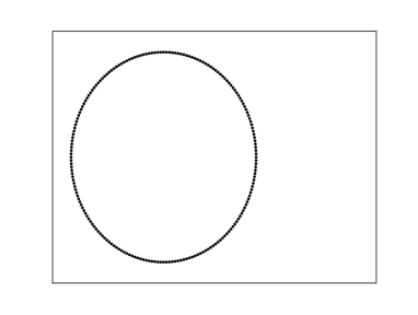
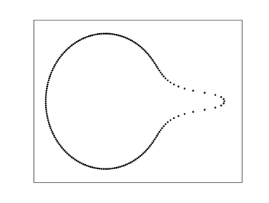
Figure 1: Figure illustrating the way in which deformation takes place in the parameterisation-independent geodesic equations for embedded curves. The initial curve is shown on the left, and the final curve is shown on the right. Since the momentum is constrained to be normal to the curve, and since the velocity is obtained by applying a smoothing kernel to the momentum, the change in the shape emerges as local stretching of the curve, and the discrete points defining the shape become separated.

These difficulties are all removed if, instead, one solves the following problem:

Definition 22 (Reparameterised curve matching problem).

Let $\overline{\boldsymbol{q}}(s;t)$ be a one-parameter family of parameterised curves in $\mathbb{R}^{2}$, with $s\in[0,1]$ being the curve parameter and $t\in[0,1]$ being the parameter for the family. Let $\overline{\boldsymbol{u}}(\boldsymbol{x};t)$ be a one-parameter family of vector fields on $\mathbb{R}^{2}$. Let $\nu$ be a vector field on $S^{1}$. We seek $\overline{\boldsymbol{q}}$, $\overline{\boldsymbol{u}}$ and $\nu$ which satisfy

$$\min_{\overline{\boldsymbol{u}},\nu}\int_{0}^{1}\frac{1}{2}\|\overline{\boldsymbol{u}}\|^{2}_{V}\operatorname{d\!}{t}$$

subject to the constraints

$$\mbox{\rm[Reconstruction relation]}\quad\frac{\partial}{\partial t}\overline{\boldsymbol{q}}(s;t) = \overline{\boldsymbol{u}}(\overline{\boldsymbol{q}}(s;t),t)+\nu(s)\frac{\partial}{\partial s}\boldsymbol{q}(s;t),$$ (57)

$$\mbox{\rm Initial state (Template)]}\quad\overline{\boldsymbol{q}}(s;0) = \overline{\boldsymbol{q}}^{A}(s),$$ (58)

$$\mbox{\rm[Final state (Target)]}\quad\overline{\boldsymbol{q}}(s;1) = \overline{\boldsymbol{q}}^{B}(s),$$ (59)

where $\|\cdot\|_{V}$ is the chosen norm which defines the space of vector fields $V$.

Lemmas 15 and 17 state that extrema of this problem can be obtained by solving the shooting problem

$$\frac{\partial}{\partial t}\overline{\boldsymbol{q}}(s;t) = \overline{\boldsymbol{u}}(\overline{\boldsymbol{q}}(s;t),t)+\nu(s)\frac{\partial}{\partial s}\overline{\boldsymbol{q}}(s;t),$$

$$\frac{\partial}{\partial t}\overline{\boldsymbol{p}}(s;t) = -\overline{\boldsymbol{p}}(s;t)\cdot\nabla\overline{\boldsymbol{u}}(\overline{\boldsymbol{q}}(s;t),t)-\frac{\partial}{\partial s}\left(\nu(s)\overline{\boldsymbol{p}}(s;t)\right),$$

$$\left\langle\boldsymbol{w},\overline{\boldsymbol{u}}(\cdot,t)\right\rangle_{V} = \int_{S^{1}}\overline{\boldsymbol{p}}(s;t)\cdot\boldsymbol{w}(\overline{\boldsymbol{q}}(s;t),t)\operatorname{d\!}{s},\qquad\forall\boldsymbol{w}\in V^{*},$$

with boundary conditions

$$\overline{\boldsymbol{q}}(s;0)=\boldsymbol{q}^{A}(s),\quad\overline{\boldsymbol{p}}(s;0)\cdot\frac{\partial}{\partial s}\boldsymbol{q}^{A}=0,\quad\overline{\boldsymbol{q}}(s;1)=\boldsymbol{q}^{B}(s).$$

The aim is to find $\nu(s)$ and normal components of $\boldsymbol{p}(s;0)$ such that these boundary conditions are satisfied. Note that in this modified problem, the boundary condition for $\boldsymbol{q}(s;1)$ is specified pointwise (i.e. there is no reparameterisation variable $\eta$ in the boundary condition). This means that the error can be described directly in terms of

$$\|\boldsymbol{q}(\cdot;1)-\boldsymbol{q}^{B}\|^{2}$$

for some chosen norm, which can be discussed in terms of measurement errors directly.

Theorem 19 then states that a solution to the problem described in Definition 1 can be reconstructed via

$$\boldsymbol{q}(s;t)=\overline{\boldsymbol{q}}(\eta(s;t),t),\quad\boldsymbol{p}(s;t)=\overline{\boldsymbol{p}}(\eta(s;t),t)\frac{\partial}{\partial s}\eta(s;t)$$

where

$$\eta(s;t)=\exp(\nu(s)t).$$

This transformation produces a equivalent shooting problem in which the end condition for $\mathbf{\overline{q}}$ is now fixed.

4 Summary and outlook

In this paper, we studied an optimal control problem on a Lie group in which the end boundary condition is specified only up to a symmetry. We showed how this problem can be transformed into a modified problem in which the end boundary condition is fixed, but an extra parameter is introduced in the reconstruction relation, and proved that the two problems are equivalent. This approach is motivated by the problem of computing a geodesic on the diffeomorphism group in the plane which takes one curve to another. The transformation gives rise to a system of equations for a parameterised curve in which the end boundary condition for each value of the parameter is fixed. This means that when a discrete approximation of the curve is used to solve this problem numerically, the end boundary condition can again be fixed exactly. In particular, when solving a shooting problem, this means that the error between the computed curve and the target curve can be computed simply by measuring the Euclidean distance between points for each value. This method extends straightforwardly to the problem of finding geodesics in the three-dimensional diffeomorphism group which take one parameterised surface to another, with the end boundary condition specified only up to reparameterisations of the target surface. This problem has many applications in, for example, biomedicine, since it allows topologically equivalent surfaces to be characterised by a momentum field distributed on the template surface. Such momentum fields exist in a linear space and so can be manipulated using linear techniques and still a topologically equivalent surface will always be obtained.

In the standard approach to planar image registration, the problem of registering a specified closed curve (called the template) at time $t=0$ to another (the target) at time $t=1$ amounts to deforming the space $\mathbb{R}^{2}$ in which the template curve is embedded until it matches the fixed target image to within a certain tolerance. Here, we considered a manifold $Q$ comprising the space of closed curves $S^{1}$ embedded into the plane $\mathbb{R}^{2}$, written as $Q=\operatorname{Emb}(S^{1},\mathbb{R}^{2})$. There are two Lie group actions available for manipulating the closed curves in this description. The action $G\times\mathbb{R}^{2}\to\mathbb{R}^{2}$ of the Lie group $G=\operatorname{Diff}(\mathbb{R}^{2})$ by composition from the left deforms the range space $\mathbb{R}^{2}$, and thereby drags along a curve embedded in it as $GQ=\operatorname{Emb}(S^{1},G\cdot\mathbb{R}^{2})$. This left action produced the singular-solution momentum map, $\mathbf{J}_{\rm Sing}$ in equation (55), which introduces the parameterisation of the closed curve by its position and momentum supported on a delta function defining the curve in $\mathbb{R}^{2}$. Under this left action of $G$, the curve preserves the initial parameterisation of its domain space in $S^{1}$, although the current positions of the $S^{1}$ labels in the plane $\mathbb{R}^{2}$ will change as the range space is transformed. Alternatively, the action $H\times S^{1}\to S^{1}$ of the Lie group $H=\operatorname{Diff}(S^{1})$ by composition from the right transforms coordinates in the domain space $S^{1}$ as $HQ=\operatorname{Emb}(H\cdot S^{1},\mathbb{R}^{2})$, while keeping the curve fixed in the range space $\mathbb{R}^{2}$.

The present paper discussed how the left action of $\operatorname{Diff}(\mathbb{R}^{2})$ and the right action of $\operatorname{Diff}(S^{1})$ on $Q=\operatorname{Emb}(S^{1},\mathbb{R}^{2})$ may complement each other in formulating a variational approach for registration of curves under large deformations. The left action of $\operatorname{Diff}(\mathbb{R}^{2})$ corresponds to deforming the curve by a time-dependent transformation of the coordinate system in which it is embedded, while leaving the parameterisation of the curve invariant. The dynamics of this deformation is formulated as an Euler-Poincaré equation for $\mathbf{J}_{\rm Sing}\in\mathfrak{X}(\mathbb{R}^{2})^{\ast}$ that results in Hamilton’s canonical equations for the momentum and position variables of the curve that comprise the singular-solution momentum map (55). This solution provides the dynamics for curves that fulfills D’Arcy Thompson’s vision of shape transformation [Tho17]. This vision underlies common practice in image registration [Beg03].

The right action of $\operatorname{Diff}(S^{1})$ corresponds to adaptively reparameterising the $S^{1}$ domain coordinates of the curve. This reparameterisation of the curve could be useful, for example, in designing numerical methods that enhance the resolution of its main features as it deforms in $\mathbb{R}^{2}$. As we have seen, this right action unlocks the parameterisation in the control problem to allow it more freedom for matching the curve shapes using an equivalent boundary value problem, without being constrained to match corresponding points along the template and target curves at the endpoint in time. As explained above, the action of $\operatorname{Diff}(S^{1})$ from the right gives us the momentum map $\mathbf{J}_{S}:T^{\ast}\operatorname{Emb}(S^{1},\mathbb{R}^{2})\rightarrow\mathfrak{X}(S)^{\ast}$, which we used to ensure that the momentum of the curve has no tangential component. This momentum map for right action is given explicitly as

$$\mathbf{J}_{S}=\boldsymbol{p}\cdot\frac{\partial}{\partial s}\boldsymbol{q}\,.$$

The two momentum maps may be assembled into a single figure as in [HM04]:

We use the compatibility of these two momentum maps proven in [HM04] to divide the curve matching problem into independent registration and reparameterisation problems, leading to the reformulation of the curve matching problem as an equivalent geodesic boundary value problem.

We are currently developing numerical algorithms for the transformed equations applied to embedded curves and surfaces. As noted in [Via09], applying a piecewise constant representation to the $q$ and $p$ variables in the untransformed equations results in a set of ordered points. When this approach is extended to the transformed equations, a finite volume method is obtained, with the extra terms taking the form of an advection term in the $q$ equation, and a continuity term in the $p$ equation, which are very well developed in the finite volume approach. We will also investigate discontinuous higher-order polynomial representations of $p$ and $q$ which lead to discontinous Galerkin methods. Since the error in the transformed problem can be quantified in terms of the Euclidean distance between points on the curve for each parameter value, the reparameterised formulation also makes it much easier to perform Bayesian studies in which one observes points on a curve with observation error from some probability distribution, and then one attempts to estimate the probability distribution for the initial conditions of $p$ (and $\nu$) for which specified points on the curve match the actual position of the observed points, after applying the time-1 flow map of the transformed geodesic equations for $p$ and $q$. This approach provides a considerably simplified observation operator to which algorithms such as the Monte Carlo Markov Chain algorithm can be applied.

Acknowledgements

We are grateful to D. C. P. Ellis, F. Gay-Balmaz, T. S. Ratiu, A. Trouvé, F.-X. Vialard and L. Younes for valuable discussions. We thank the Royal Society of London Wolfson Award Scheme for partial support during the course of this work.

References

- [BCHM00] A. M. Bloch, P. E. Crouch, D. D. Holm, and J. E. Marsden. An optimal control formulation for inviscid incompressible fluid flow. In Proc. CDC IEEE, volume 39, pages 1273–1279, 2000.
- [BCMR98] A. M. Bloch, P. E. Crouch, J. E. Marsden, and T. S. Ratiu. Discrete rigid body dynamics and optimal control. In Proc. CDC IEEE, 1998.
- [Beg03] M. F. Beg. Variational and Computational Methods for Flows of Diffeomorphisms in Image Matching and Growth in Computational Anatomy. PhD thesis, Johns Hopkins University, 2003.
- [CH09] C. J. Cotter and D. D. Holm. Continuous and discrete Clebsch variational principles. Found. Comput. Math., 9(2):221–242, 2009.
- [Cot08] C. J. Cotter. The variational particle-mesh method for matching curves. J. Phys. A: Math. Theor., 41:344003, 2008.
- [CY01] V. Camion and L. Younes. Geodesic interpolating splines. In M. Figueiredo, J. Zerubia, and A. K. Jain, editors, EMMCVPR 2001, volume 2134 of Lecture Notes in Computer Sciences. Springer, 2001.
- [GTY04] J. Glaunes, A. Trouvé, and L. Younes. Diffeomorphic matching of distributions: A new approach for unlabelled point-sets and sub-manifolds matching. In IEEE Computer Society Conference on Computer Vision and Pattern Recognition, volume 2, pages 712–718, 2004.
- [HM04] D. D. Holm and J. E. Marsden. Momentum maps and measure valued solutions of the Euler-Poincaré equations for the diffeomorphism group. Progr. Math., 232:203–235, 2004. http://arxiv.org/abs/nlin.CD/0312048.
- [Hol09] D. D. Holm. Geometric Mechanics, Part II: Translating and Rolling, chapter 1. Imperial College Press, London, 2009.
- [MM06] R. I. McLachlan and S. Marsland. The Kelvin-Helmholtz instability of momentum sheets in the Euler equations for planar diffeomorphisms. SIAM Journal on Applied Dynamical Systems, 5(4), 2006.
- [MMS06] A. Mills, S. Marsland, and T. Shardlow. Biomedical Image Registration, chapter Computing the Geodesic Interpolating Spline, pages 169–177. Springer, 2006.
- [She94] J. R. Shewchuk. An introduction to the conjugate gradient method without the agonizing pain. www.cs.cmu.edu/\~{}quake-papers/painless-conjugate-gradient.pdf, 1994.
- [Tho17] D’A. Thompson. On Growth and Form. 1917.
- [VG05] Marc Vaillant and Joan Glaunes. Surface matching via currents. In IPMI, pages 381–392, 2005.
- [Via09] F.-X. Vialard. Approche Hamiltonienne Pour les Espaces de Formes Dans le Cadre des Diffèomorphismes: Du Problème de Recalage d’Images Discontinues à un Modèle Stochastique de Croissance de Formes. PhD thesis, Ecole Normale Supéreure de Cachan, 2009.