Black Hole Spin and the Radio Loud/Quiet Dichotomy of Active Galactic Nuclei

Abstract

Radio loud active galactic nuclei (AGN) are on average 1000 times brighter in the radio band compared to radio quiet AGN. We investigate whether this radio loud/quiet dichotomy can be due to differences in the spin of the central black holes that power the radio-emitting jets. Using general relativistic magnetohydrodynamic simulations, we construct steady state axisymmetric numerical models for a wide range of black hole spins (dimensionless spin parameter $0.1\leq a\leq 0.9999$) and a variety of jet geometries. We assume that the total magnetic flux through the black hole horizon at radius $r_{\rm H}(a)$ is held constant. If the black hole is surrounded by a thin accretion disk, we find that the total black hole power output depends approximately quadratically on the angular frequency of the hole, $P\propto\Omega_{\rm H}^{2}\propto(a/r_{\rm H})^{2}$. We conclude that, in this scenario, differences in the black hole spin can produce power variations of only a few tens at most. However, if the disk is thick such that the jet subtends a narrow solid angle around the polar axis, then the power dependence becomes much steeper, $P\propto\Omega_{\rm H}^{4}$ or even $\propto\Omega_{\rm H}^{6}$. Power variations of $1000$ are then possible for realistic black hole spin distributions. We derive an analytic solution that accurately reproduces the steeper scaling of jet power with $\Omega_{\rm H}$, and we provide a numerical fitting formula that reproduces all our simulation results. We discuss other physical effects that might contribute to the observed radio loud/quiet dichotomy of AGN.

1. Introduction

The first active galactic nuclei (AGN) were discovered through radio emission associated with their relativistic jets. However, it soon became clear that not all AGN have powerful radio jets; in fact, only about 10% of quasars do. The evidence for a dichotomy between radio loud and radio quiet AGN has become stronger over the years, culminating in the impressive demonstration by Sikora, Stawarz, & Lasota (2007) that two very distinct populations of AGN are clearly visible when radio luminosities $L_{R}$ of AGN are plotted against optical luminosities $L_{B}$. For a given value of $L_{B}$, these authors show that $L_{R}$ of radio loud AGN is $\sim 10^{3}{-}10^{4}$ times greater than that of radio quiet AGN. Also, the two populations follow two well-separated tracks on the plot.

The origin of the radio loud/quiet dichotomy has been much discussed in the literature. At Eddington ratios $\lambda=L_{\rm bol}/L_{\rm Edd}\sim 10L_{B}/L_{\rm Edd}>0.01$, where $L_{\rm bol}$ is the bolometric luminosity of the AGN and $L_{\rm Edd}$ is its Eddington luminosity, a likely explanation for the dichotomy (Ho et al., 2000; Sikora et al., 2007) is that these systems accrete via a standard thin accretion disk. Jet production is then expected to be intermittent, as found to be the case in black hole (BH) X-ray binaries (Fender et al. 2004). However, the existence of two distinct populations for $\lambda<0.01$ is harder to explain. Even at these low luminosities, the radio loudness parameter $R=L_{\rm 5\ GHz}/L_{B}$ of the radio loud population is at least a factor of $10^{3}$ times larger than that of the radio quiet population. However, at low values of $\lambda$, BH X-ray binaries typically are in a hard spectral state associated with an advection-dominated accretion flow (ADAF, Narayan & McClintock 2008), and in this state, all BH X-ray binaries are radio loud (Fender et al., 2004). Why then do AGN with similar values of $\lambda$ have a radio loud/quiet dichotomy?

One possible explanation is that radio loud objects are driven by a central BH with a large spin which produces a jet by the Blandford-Znajek (BZ) mechanism (Blandford & Znajek, 1977, hereafter, BZ77). This is referred to as the spin paradigm (Blandford, 1990; Wilson & Colbert, 1995; Blandford, 1999), which is in contrast to the accretion paradigm which states that the BH mass and mass accretion rate determine the jet power (Blandford & Rees, 1974, 1992). These different paradigms plausibly operate together to some degree (Begelman et al., 1984; Meier, 2002). The spin paradigm has been invoked to explain the observed correlation between jet and accretion power in elliptical galaxies (Allen et al., 2006) by combining an ADAF accretion model with the BZ effect (Nemmen et al., 2007; Benson & Babul, 2009). In terms of the dimensionless spin parameter $a=J/GM^{2}$, where $M$ and $J$ are the mass and angular momentum of the BH, it is found that one requires $a\gtrsim 0.9$ to explain the correlation. The dichotomy in the power and spatial distribution of emission in Fanaroff-Riley classes 1 and 2 (FR 1 and FR 2) radio galaxies may also be explained by the spin paradigm (Baum et al., 1995).

The radio loud/quiet dichotomy in AGN (Kellermann et al., 1989; Moderski et al., 1998; Ivezić et al., 2004) has been explained in terms of an in situ trigger for relativistic jets (Meier et al., 1997). It could also be explained by the differences in the evolutionary stages at which we observe the objects (Blundell, 2008) coupled with the episodic activity of the AGN evidenced by the change or precession of jet orientation (Steenbrugge & Blundell, 2008; Steenbrugge et al., 2008, 2010). However, another possibility is that the two AGN populations have different merger and accretion histories which lead to different BH spins. Recent observations show that, for $\lambda<0.01$, all radio loud AGN reside in elliptical galaxies, whereas radio quiet AGN live mostly in spirals (Sikora et al., 2007). Volonteri, Sikora, & Lasota (2007) explored a number of scenarios for the formation of ellipticals and spirals and showed that it is plausible for the nuclear BHs in spirals to have lower spins than those in ellipticals. This suggests that the spin paradigm may explain the radio loud/quiet dichotomy.

The main problem with this explanation is that the difference in radio loudness between the radio loud and radio quiet populations is a factor of $10^{3}$ (Sikora et al., 2007). This is a strikingly large difference. According to the accretion or spin paradigms, relativistic jets are produced by magnetic outflows from either the inner region of the disk or the spinning BH. The power in the disk outflow is expected to be proportional to the disk luminosity, which leaves no room for a radio loud/quiet dichotomy, so we will ignore this possibility. The power from the BH does depend on the spin parameter, and we will focus on this. However, the analytical model of BZ77 indicates that the jet power $P$ varies only as $a^{2}$ for fixed magnetic flux threading the horizon. If such a weak variation is to produce a difference of $10^{3}$ in radio power, we need $a$ in the two populations to differ by a factor $\sim 30$, which does not seem plausible given likely merger histories (Hughes & Blandford, 2003; Gammie et al., 2004). More plausible is a factor $\sim 3$ difference in the median values of $a$ in the two populations (e.g., see Volonteri et al. 2007), but this will produce only a factor $\sim 10$ difference in jet power, not $10^{3}$.

The BZ77 scaling for power, $P\propto a^{2}$, was derived in the limit $a\ll 1$, for a razor-thin disk, assuming the magnetic flux threading the BH is independent of $a$. Recent analytical and numerical work by Tanabe & Nagataki (2008) show that, for a BH threaded by a split monopole magnetic field, $P$ increases as $a^{4}$ at large values of $a$ when higher-order corrections are included. However, the analytical model worked out by these authors only gives a factor of two increase in power above the BZ77 result even at $a=1$. Their numerical simulations achieve a slightly steeper scaling, but still only a factor of four above the BZ77 result at $a=1$. In any case, their work hints that a much steeper dependence of power on $a$ occurs as $a\to 1$. Are there other effects that can introduce an even steeper dependence on $a$?

General relativistic magnetohydrodynamic simulations of accretion disks by McKinney (2005b) showed that for $a\gtrsim 0.5$ the jet power varies as steeply as the fourth power of the BH angular rotation rate, i.e., $P\propto\Omega_{\rm H}^{4}$, where $\Omega_{\rm H}\propto a/r_{\rm H}$ and $r_{\rm H}$ is the radius of the horizon. Compared to the scaling $P\propto a^{4}$, the scaling $P\propto\Omega_{\rm H}^{4}$ introduces an additional factor of $16$ due to the division by $r_{\rm H}$, since $r_{\rm H}$ decreases from $2M$ to $M$ as $a$ varies from $0$ to $1$. McKinney (2005b) also finds that the power output of the entire BH has a shallower dependence on $\Omega_{\rm H}$ compared to the power output of the jet, which subtends a small solid angle above the disk and corona. This suggests that changes in the solid angle subtended by the jet (via changes in the disk thickness) could change the steepness of the power output as a function of $a$.

Since the scaling of $P$ with BH spin is important for jet studies, we have explored this issue in detail using general relativistic magnetohydrodynamic numerical simulations. We consider a variety of geometries for the shape of the jet to see if we can come up with any scenario in which jet power could change by a large factor for a modest variation in $a$. We show that the most favorable scenario is a BH surrounded by a thick accretion flow with an angular thickness $H/R\sim 1$. We show that in this case the power output into a polar jet has a steep dependence on the spin, $P\propto\Omega_{\rm H}^{4}$, and that the scaling steepens to $P\propto\Omega_{\rm H}^{6}$ for even thicker disks. Hence, we confirm the basic result found by McKinney (2005b) of a steep dependence of jet power on $a$ at high latitudes above the disk. We suggest that this strong dependence may explain the radio loud/quiet dichotomy in AGN.

Our numerical setup is described in §2. The results for BHs with razor-thin disks are presented in §3.1, and for jets from BHs with thick disks in §3.2. We discuss the results in the context of the AGN radio loud/quiet dichotomy in §4, and conclude in §5. We work with Heaviside-Lorentzian units and set $c=G=1$.

2. Numerical Setup

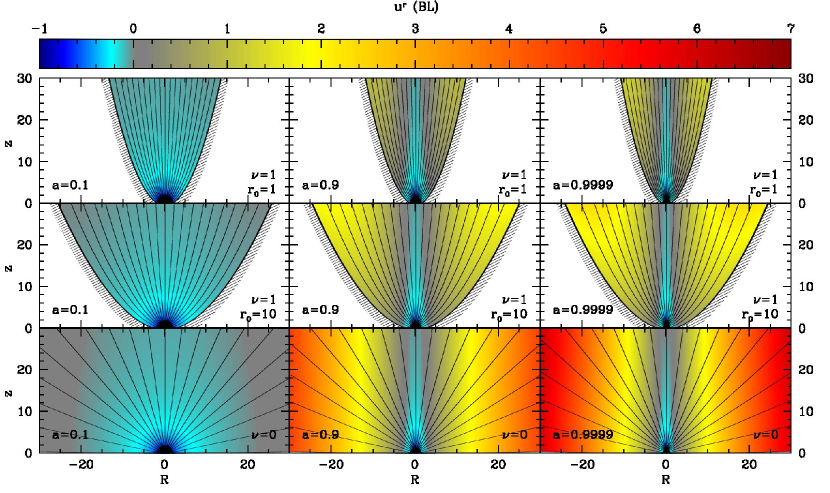
Figure 1.— Meridional cuts through a selection of numerical jets in the force-free approximation, i.e., neglecting plasma inertia. The color-coded radial four-velocity $u^{r}$ (as measured in Boyer-Lindquist coordinates, see legend) is shown overlaid with poloidal field lines (thin black lines which correspond to $\Psi^{1/2}=0,0.2,\dots,1$). The jets are confined by collimating walls (thick black lines). The left-most column of panels shows models with a low BH spin ($a=0.1$), the right-most column models with a fast spin ($a=0.9999$), and the middle column models with an in-between spin ($a=0.9$). The top row of panels shows the most collimated paraboloidal models ($\nu=1,~{}r_{0}=M$), the bottom row non-collimating monopolar models ($\nu=0$), and the middle row models that are monopole-like until $r\simeq{}r_{0}=10M$, beyond which they become paraboloidal ($\nu=1,r_{0}=10M$).

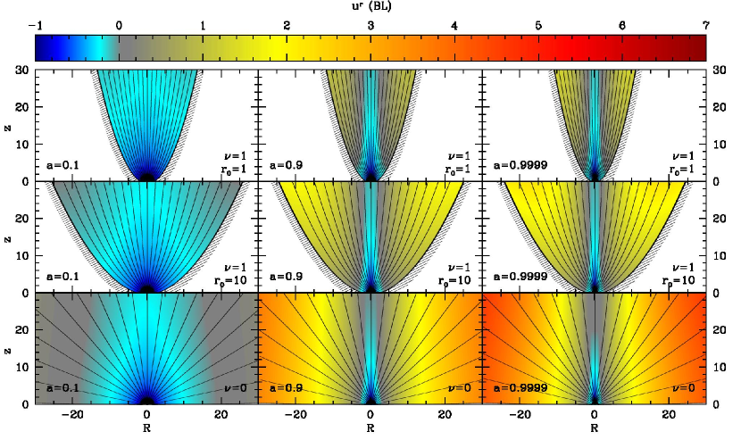
Figure 2.— Meridional cuts through a selection of numerical magnetohydrodynamic, i.e., mass-loaded, jets. These may be directly compared to the force-free (i.e., neglecting plasma inertia) jet models shown in Figure 1: the jet geometries are the same, but the jets here include mass-loading. While the field line shape changes little from Figure 1, the introduction of mass-loading does lead to clear differences in the velocity. (i) The inflow near the BH is faster in mass-loaded jets ($u^{r}$ is more negative in blue regions) due to the gravitational pull of the BH. (ii) The outflow from the BH in monopolar jets (the bottom set of panels) is slower than in the corresponding force-free simulations. Nevertheless, the jet powers are nearly the same in the two sets of models.

It is known that a highly magnetized relativistic jet does not easily self-collimate. For instance, the equilibrium field configuration around an isolated spinning BH threaded by a magnetic field (sourced by external currents) takes the form of a split monopole (BZ77). Only extremely close to the polar axis is any evidence of self-collimation present (Tchekhovskoy et al., 2009a). Therefore, in order to produce a jet which collimates most of the energy output from the BH, it is necessary to introduce an external confining medium. The confining agent may be the gas in an accretion disk, a corona, or a wind emerging from the inner regions of the disk. Ideally, one should numerically simulate both the jet and the confining medium, but this is numerically very challenging. Instead, we follow the more usual approach (e.g., Komissarov et al. 2007; Tchekhovskoy et al. 2009b) of introducing a rigid axisymmetric wall with a prescribed shape and requiring the jet to lie inside the wall. The shape of the wall is set by two parameters:

1. An index $\nu$ which sets the asymptotic poloidal field line shape, as described below. This parameter ranges from $\nu=0$, which corresponds to a monopole field geometry, to $\nu=1$, which corresponds to a paraboloidal jet. In a real system, $\nu$ would be set by the radial pressure profile of the confining medium. Plausible values are in the range $\nu\sim 0.5{-}1$ (Tchekhovskoy et al., 2008).

2. A transition radius $r_{0}$ which is defined such that for $r\lesssim{}r_{0}$ the jet is monopolar and for $r\gtrsim{}r_{0}$ it switches to the shape prescribed by $\nu$. The parameter $r_{0}$ allows us to consider situations in which confinement operates only beyond a certain distance from the BH.

In terms of these two parameters, the wall has the following shape in polar $(r,\theta)$ coordinates in the Boyer-Lindquist frame:

$$1-\cos\theta=\left(\frac{r+r_{0}}{r_{\rm H}+r_{0}}\right)^{-\nu},\qquad r_{\rm H}=M\left[1+(1-a^{2})^{1/2}\right],$$ (1)

where $r_{\rm H}$ is the radius of the BH horizon. For $r\ll{}r_{0}$, $(1-\cos\theta)\ll 1$, so $\theta\approx\pi/2$, i.e., the wall lies along the equatorial plane, as for a split monopole. For $r\gg(r_{\rm H},r_{0})$, $\theta\propto{}r^{-\nu/2}$, which corresponds to a generalized paraboloid. Note that, in all these models, the wall meets the horizon at the equator. In effect, this means we assume a razor-thin disk which subtends zero solid angle at the BH. In §3.2 we discuss the case of geometrically thick disks.

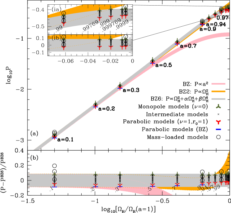
Figure 3.— Jet power output of various models as a function of dimensionless BH horizon spin frequency $\omega_{\rm H}=\Omega_{\rm H}/\Omega_{\rm H}(a=1)$ (equation 5). Different models are shown with different symbols (see legend). For reference, the following values of BH spin, $a=\{0.2,0.5,0.9,1\}$, correspond to approximately the following values of $\omega_{\rm H}$: $\{0.1,0.27,0.63,1\}$. [Upper panel (a)]: Logarithm of jet power. [Lower panel (b)]: Fractional deviation of the numerical jet power from the BZ6 formula (9). [Insets (ia) and (ib)] Blow-ups of panels (a) and (b) for high values of BH spin. The values of the BH spin $a$ are shown as labels next to data points. The three colored stripes (see legend) correspond to the original BZ77 scaling (equation 4), the BZ2 scaling (equation 7), and the BZ6 scaling (equation 9). The second-order BZ2 scaling (7) follows the numerical results very well except for values of $a$ close to unity. The BZ6 scaling (9) matches the numerical data well at all values of $a$. For each $a$, the monopolar model ($\nu=0$) has the maximum power and the paraboloidal model has the least power. However, the difference is only $\sim 20\%$

Having picked the shape of the wall, we choose the poloidal flux function of the initial magnetic field configuration to be

$$\Psi=\left(\frac{r+r_{0}}{r_{\rm H}+r_{0}}\right)^{\nu}(1-\cos\theta).$$ (2)

Note that $\Psi$ is conserved along each field line, and $\Phi=2\pi\Psi(r,\theta)$ is the poloidal magnetic flux through a toroidal ring at $(r,\theta)$. By construction, equation (2) corresponds to a total flux of $\Phi_{\rm tot}=2\pi$ in the jet. In this model $\Phi_{\rm tot}$ does not depend upon spin, so the amount of magnetic flux threading the BH is fixed for different spins. The outermost field line, defined by $\Psi=1$, follows the shape of the wall. This particular field line is always located at the wall because of our boundary conditions. Interior field lines, however, are free to move once the simulation begins and do experience minor shifts in the poloidal direction. The initial magnetic field has no toroidal component.

There are no known exact solutions for the magnetosphere of a spinning BH. However, the poloidal field configurations given in equation (2) are sufficiently close to the true solutions that their initial relaxation when the simulation starts is rather mild. Only two linearly independent analytic solutions have been obtained for a non-spinning BH: one corresponds to a monopolar field geometry and is given by equation (2) with $\nu=0$, while the other is the following BZ77 solution for a paraboloidal field,

$$\Psi=\frac{(r/r_{\rm H}-1)(1-\cos\theta)-(1+\cos\theta)\log(1+\cos\theta)}{2\log 2}+1.$$ (3)

Note that the split-monopole solution applies to the entire space exterior to the horizon, whereas the paraboloidal solution only applies to the field lines attached to the BH (see McKinney & Narayan 2007b for a numerical paraboloidal solution that applies to the whole space). Any linear combination of the monopolar and paraboloidal solutions is also a solution (see, e.g., Beskin, 2009). The BZ77 paraboloidal solution (3) is very similar to the approximate solution (2) for the case $\nu=1$, and this is our reason for focusing on the simpler model (2), with $\nu$ varying over the range 0 to 1. For completeness, we have also run simulations using the BZ77 field geometry (3) to initialize the calculations (along with the appropriate choice of the wall shape, obtained by setting $\Psi=1$ in this equation).

We performed the simulations using the general relativistic (GR) MHD code HARM (Gammie et al., 2003; McKinney & Gammie, 2004; McKinney, 2006b, a; Noble et al., 2006) using Kerr-Schild coordinates in the Kerr metric; the code includes a number of recent improvements (Mignone & McKinney 2007; Tchekhovskoy et al. 2007, 2008, 2009a). Most of the simulations were done in the force-free approximation, which assumes that the plasma is infinitely magnetized and has negligible inertia. Within this approximation, the problem is fully defined by specifying just the BH spin and the shape of the wall. Figure 1 shows results from several representative simulations.

Real relativistic jets are of course not perfectly force-free; in fact, they are expected to deviate substantially from this approximation at large distances from the BH. However, all relativistic MHD jets that have $\gamma\gg 1$ are highly magnetized near the BH, and here they are expected to be well represented by force-free solutions (BZ77). Moreover, the power that a relativistic jet carries is determined entirely by the initial force-free zone. Therefore, we expect numerical results on the jet power from a force-free simulation to agree very well with the power for an MHD jet with inertia.

To verify this expectation, we have repeated some of our force-free simulations in the MHD limit, in which the jet is mass-loaded with a finite amount of plasma (details given below). Figure 2 shows some results. As expected, we find that the asymptotic Lorentz factor $\gamma$ of the jet does depend on mass-loading: a force-free jet accelerates without limit (Tchekhovskoy et al., 2008), whereas an MHD jet asymptotes to a finite $\gamma$ which is determined by the initial magnetization of the jet. However, we find that the jet power, the primary quantity of interest to us in this paper, is not sensitive to mass-loading so long as the jet is relativistic, i.e., so long as the jet is initially force-free near the BH.

MHD jets are more complicated and require more parameters to be specified compared to force-free jets. In particular, the results depend on the details of mass-loading at the base of the jet. Highly magnetized jets accelerate because the magnetic energy flux, which dominates the energy budget at the base of the jet, is converted to kinetic energy flux of the plasma as the jet flows out. The ratio of magnetic to kinetic energy flux at the base of the jet determines the asymptotic Lorentz factor (Begelman & Li, 1994; Komissarov et al., 2009; Tchekhovskoy et al., 2009a, b). Observations suggest a characteristic value for the Lorentz factor of AGN jets $\gamma_{\rm AGN}\sim 25$ (Jorstad et al., 2005). We choose the following simple prescription for the mass-loading of our numerical MHD jets to roughly match this value. We impose a floor on the co-moving rest-mass density of the jet $\rho_{\rm floor}$ such that whenever the density falls below this value, we add mass in the co-moving frame of the plasma. This simple floor model is a convenient way of numerically representing more complicated (and poorly understood) processes that are responsible for the mass-loading of jets in AGN. The value of $\rho_{\rm floor}$ is selected such that the rest mass energy density $\rho_{\rm floor}c^{2}$ is equal to a fraction $1/\gamma_{\rm AGN}$ of the co-moving magnetic energy density $\epsilon_{m}$: $\rho_{\rm floor}c^{2}=\epsilon_{\rm m}/\gamma_{\rm AGN}$. Thus, our floor model ensures that the ratio of $\epsilon_{m}$ to $\rho_{\rm floor}c^{2}$ does not exceed $\gamma_{\rm AGN}$, thereby making sure that the maximum Lorentz factor of our jets is close to the required value. We note that while our procedure is Lorentz invariant, it might not correspond to a physical process that operates in AGN, e.g., photon annihilation from the accretion disk (Phinney, 1983).

The code uses internal coordinates $(x_{1},x_{2})$ that are uniformly sampled with $512\times 128$ grid cells. The internal coordinates are mapped to the physical coordinates $(r,\theta)$ via $r/M=R_{0}+\exp(x_{1})$ and $x_{2}={\rm{}sign}(\Psi)\left|\Psi\right|^{1/2}$. The computational domain extends radially from the inner boundary at $r_{\rm{}in}=0.6M+0.4r_{\rm H}$ to the outer boundary at $r_{\rm{}out}=10^{4}M$. We apply absorbing (outflow) boundary conditions at each of these boundaries. In the $\theta$-direction, the computational domain extends from the polar axis at $x_{2}=0$, where we use the usual polar boundary conditions, to the jet boundary $x_{2}=1$, where we place the wall. At the wall, we outflow (copy) the components of velocity and magnetic field that are parallel to the wall, and mirror the perpendicular components (Tchekhovskoy et al., 2009a). For a given BH spin and grid resolution, we choose the value of $R_{0}$ such that there are $7$ to $10$ grid cells between $r_{\rm{}in}$ and $r_{\rm H}$. This ensures that the inner radial grid boundary $r=r_{\rm{}in}$ is causally disconnected from the region outside the BH horizon.

At time $t=0$ we initialize the simulation with a purely poloidal field configuration as described in equation (2) (or equation 3 in the case of the BZ77 paraboloidal model) and we run the simulation until $t_{\rm{}f}={\rm{}max}(100M,20/\Omega_{\rm H},10r_{0})$. Because of the dragging of frames by the spinning BH, the magnetic field develops a toroidal component which propagates out along field lines at nearly the speed of light. Behind this outgoing wave, the solution settles down to a steady state and we study the properties of this steady solution. We have verified by running selected simulations for $10$ times longer than our fiducial $t_{\rm{}f}$ that the near-BH regions of our numerical solutions have truly reached steady state.

3. Results

3.1. Power Output of Black Holes with Razor-thin Disks

As explained below equation (1), all our jet models correspond to the case of a razor-thin disk. We describe here the results we obtain for these models.

BZ77 showed that the luminosity of a force-free jet from a slowly spinning BH ($a\ll 1$), embedded in a regular magnetic field with a fixed total flux (sourced by toroidal currents in a razor-thin disk), is proportional to the square of the BH spin and the square of the magnetic field strength at the horizon. If we include the length scale of the horizon $2M$ to obtain the correct dimensions, we may write (the choice of the numerical prefactor will become clear below)

$$P^{\rm{}BZ}(a)=k\Phi_{\rm{}tot}^{2}\frac{a^{2}}{16M^{2}},$$ (4)

where $\Phi_{\rm tot}\propto{}B{}M^{2}$ is the total poloidal magnetic flux in the jet, and $k$ is a constant which depends on the field geometry, e.g., $k=k_{\rm mono}=(6\pi)^{-1}\approx 0.054$ for a monopolar field ($\nu=0$) and $k=k_{\rm para}\approx 0.044$ for the paraboloidal BZ77 geometry (equation 3). We refer to equation (4) as the original BZ77 scaling.

Because equation (4) was derived in the limit $a\ll 1$, it can be extended to larger values of $a$ in several ways. In particular, we could replace the length scale $2M$ by the horizon scale $r_{\rm H}$, where $r_{\rm H}$ is defined in equation (1). In fact, this is a more natural scaling since the angular frequency of the BH,

$$\Omega_{\rm H}(a)=\frac{a}{2r_{\rm H}(a)},$$ (5)

clearly plays an important role in determining the power in the jet at the horizon (BZ77; McKinney & Gammie 2004). BZ77 found that, for a fixed field strength at the BH horizon, the power in the outflow obeys (BZ77; McKinney & Gammie 2004):

$$P\propto\Omega(\Omega_{\rm H}-\Omega)\bigr{|}_{r=r_{\rm H}}\propto\Omega_{\rm H}^{2},$$ (6)

where, based on dimensional argument, the field line angular frequency, $\Omega$, is proportional to $\Omega_{\rm H}$ (see Appendix A). Numerical simulations by Komissarov (2001) showed that the BZ77 effect achieves maximum efficiency when $\Omega\approx\Omega_{\rm H}/2$. The result was found to be true for $a=\{0.1,0.5,0.9\}$, demonstrating that this result is valid even in the non-linear regime. Now, replacing the length scale $2M$ with the horizon scale $r_{\rm H}$ in the expression for power (4), we obtain:

$$P^{\rm{}BZ2}(\Omega_{\rm H}){}=k\Phi_{\rm{}tot}^{2}\Omega_{\rm H}^{2}.$$ (7)

In Appendix A we derive this formula analytically from first principles. The scaling of jet power (7) was confirmed in the numerical simulations by Krasnopolsky (private communication). In general, $k$ is a constant factor whose value depends on the field geometry near the BH. For a slowly spinning BH, $a\approx 4\Omega_{\rm H}M$, and equation (7) reduces to the standard BZ77 scaling which was derived in the limit $a\ll 1$. However, as expected from the above discussion and as we will confirm shortly, equation (7) is a better approximation for higher spins and is quite accurate up to $a\approx 0.95$, beyond which it requires a modest correction. We refer to equation (7) as the modified second-order BZ77 scaling, or simply the BZ2 scaling. We classify the order of a scaling by the maximum power of $\Omega_{\rm H}$ up to which the scaling maintains its accuracy. As we will see below, for large spins $a\simeq 1$, scalings higher than the $2$nd order are required to obtain good agreement with the numerical results.

Tanabe & Nagataki (2008) found $4$th order corrections to the BH power output by performing the expansion in powers of BH spin $a$. As we have argued, a more accurate expansion is in powers of the BH rotational frequency $\Omega_{\rm H}$ (equation 5). Recast in powers of $\Omega_{\rm H}$, the Tanabe & Nagataki (2008) expansion becomes:

$$P^{\rm BZ4}(\Omega_{\rm H})\approx k\Phi_{\rm{}tot}^{2}(\Omega_{\rm H}^{2}+\alpha\Omega_{\rm H}^{4}),$$ (8)

where the $4$th-order coefficient $\alpha=8\left(67-6\pi^{2}\right)/45\approx 1.38$. We analytically derive this formula from first principles in Appendix B. Note that the expansion only contains even powers of $\Omega_{\rm H}$ since the power is independent of the sense of BH rotation. As we will see, this $4$th order correction agrees well with the numerical results and is an improvement over the $2$nd order formula (7). However, at high spins, $a\gtrsim 0.99$, even the formula (8) becomes inaccurate. Below we present a more accurate $6$th order formula (see equation 9).

We have performed numerical simulations of force-free jets confined by a rigid wall (as described in §2) for a wide range of field geometries and BH spins. We numerically explored all possible combinations of $\nu=\{0,\linebreak[0]0.25,\linebreak[0]0.5,\linebreak[0]0.75,\linebreak[0]1\}$, $r_{0}=M\times\{0,\linebreak[0]1,\linebreak[0]5,\linebreak[0]10,\linebreak[0]100\}$ and $a=\{0.1,\linebreak[0]0.2,\linebreak[0]0.3,\linebreak[0]0.5,\linebreak[0]0.7,\linebreak[0]0.9,\linebreak[0]0.94,\linebreak[0]0.97,\linebreak[0]0.99,\linebreak[0]0.99769,0.999,\linebreak[0]0.999769,\linebreak[0]0.9999\}$. We also performed simulations in which we started the field with the paraboloidal BZ77 geometry (3). In addition to force-free simulations, which neglect plasma inertia, we have also performed MHD (mass-loaded) simulations for selected field geometries and spins: $\nu=\{0,\linebreak[0]1\}$, $r_{0}=M\times\{0,\linebreak[0]1,\linebreak[0]10\}$ and $a=\{0.1,\linebreak[0]0.9,\linebreak[0]0.99,\linebreak[0]0.9999\}$.

Figures 1 and 2 illustrate the effect of the shape parameter $\nu$ and the transition radius $r_{0}$ on the jet geometry. The larger the value of $\nu$, the more collimated is the jet. The larger the value of $r_{0}$, the more monopolar-like is the jet geometry near the BH. The shape of the poloidal field lines weakly depends on the BH spin: careful examination of the figures reveals that the field lines tend to come closer to the jet axis for faster spins, and this effect is largest near the BH horizon. The magnetosphere clearly divides into an outflow region ($u^{r}>0$) and an inflow region ($u^{r}<0$) separated by a stagnation surface at which the radial velocity vanishes. This is similar to what is seen in simulations of magnetized turbulent tori around spinning BHs (McKinney & Gammie, 2004; McKinney, 2006b; McKinney & Blandford, 2009).

Figure 3 shows the numerically measured power output of all our models as a function of the BH horizon frequency $\Omega_{\rm H}$ (defined in eq 5). The colored stripes correspond to the three scalings: BZ (equation 4), BZ2 (equation 7), and BZ6 (equation 9). For a given BH spin, a monopolar field geometry ($\nu=0$) produces a more powerful jet since it has a larger value of the pre-factor $k_{\rm{}mono}\approx 0.054$ compared to the paraboloidal BZ77 geometry (equation 3, $k_{\rm{}para}\approx 0.044$, BZ77). This difference in $k$ determines the width of the colored stripes in Fig. 3. The model given in equation (2) with $\nu=1$ is close to the BZ77 paraboloidal solution and has nearly the same power. Models with intermediate values of $\nu$ ($0<\nu<1$) or with non-zero values of $r_{0}$ have power output intermediate between the two limiting models and form the vertical clusters of numerical points at each $a$ in Figure 3. Independent of the value of $\nu$, we find that jets with $r_{0}$ much larger than the outer “light cylinder” radius $\simeq 1/\Omega_{\rm H}$ have luminosities very similar to that of a monopolar jet.

As expected, for small BH spins, $a\lesssim 0.3$, both the original BZ77 scaling (equation 4) and the second order BZ2 scaling (equation 7) agree well with the numerical results. As we go to higher spins, the BZ2 scaling (7) continues to follow the simulation data points accurately, while the original BZ77 scaling (4) under-predicts the power (e.g., by a factor $\approx 3$ at $a=0.99$).

Careful examination of Fig. 3a and especially of the inset Fig. 3ia, which shows a blowup of the $a\to 1$ region of the plot, reveals a flattening in the numerical data points at spin values $a\gtrsim 0.95$: the BZ2 formula (7) over-predicts the jet luminosity by about $25\%$ as $a\to 1$ (in agreement with R. Krasnopolsky, private communication). It is not clear that this corner of parameter space is particularly relevant for astrophysics, nor is the effect very large. Nevertheless, for completeness we note that the flattening of the jet power can be well-modeled by including higher-order corrections to the BZ2 formula (7), e.g., by the BZ6 formula which we derive in Appendix C. We give here a simplified version of this formula:

$$P^{\rm{}BZ6}(\Omega_{\rm H})\approx k\Phi_{\rm{}tot}^{2}(\Omega_{\rm H}^{2}+\alpha\Omega_{\rm H}^{4}+\beta\Omega_{\rm H}^{6}),$$ (9)

where the value of $\alpha$ is determined analytically, $\alpha\approx 1.38$ (same as in the BZ4 expansion, equation 8) and $\beta$ is found numerically by least-square fitting equation (9) to the full BZ6 analytic formula derived in Appendix C: $\beta\approx-9.2$. The gray stripe in Figure 3 compares this formula to our numerical results for the full range of models. Higher order corrections have no effect at small spin values (the gray and light red stripes lie on top of each other) but do a good job of reproducing the flattening in the jet luminosity at spin values $a\gtrsim{}0.95$ and the slight but systematic increase in the power output of the numerical jets above the light red stripe at $a\lesssim 0.9$ (this increase is especially apparent in Figure 3b). In anticipation of future discussion, it is useful to express the power at low spin in terms of the maximum achievable power at $a=1$:

$$P(a)\simeq 0.32a^{2}P(a=1),\quad a\lesssim 0.3.$$ (10)

We now look into the origin of the differences in the power outputs of the various model jets, as well as of the numerical trends discussed above. We focus on two limiting cases: monopolar jet ($\nu=0$) and paraboloidal jet ($\nu=1$, $r_{0}=1$).

First, let us recast the power output of the jet in a convenient form. In a stationary axisymmetric force-free flow, several quantities are conserved along poloidal field lines (defined by $\Psi={\rm{}const}$). Two of these are the field line angular velocity $\Omega(\Psi)$ and the enclosed poloidal current $I(\Psi)$ (Tchekhovskoy et al., 2008). The power output of a force-free jet may be written as the integral of the outward Poynting flux $S^{r}\equiv-\Omega B^{r}B_{\varphi}$ over a spherical jet cross-section. In this notation, the lower component of the toroidal magnetic field is up to a numerical factor the enclosed poloidal current, $-2\pi B_{\varphi}\equiv I(\Psi)$. Using this notation, which is very similar in appearance and meaning to the usual special relativistic notation, we obtain the total power output of the BH by integrating over the surface of the BH (see also BZ77):

$$P=\iint{}S^{r}\,dA=2\int_{0}^{\pi/2}\Omega B^{r}I\,dA=2\int_{0}^{1}\Omega(\Psi)I(\Psi)\,d\Psi,$$ (11)

where the field strength $B^{r}$ times the area element $dA$ gives the magnetic flux through that area, $d\Phi=2\pi d\Psi=B^{r}\,dA$, and the numerical factor of $2$ accounts for the two hemispheres of the BH.

Figure 4 shows for a monopolar jet the angular profiles of angular velocity $\omega=\Omega/\Omega_{\rm H}$, enclosed poloidal current $i=I/\Omega_{\rm H}$, and power output $p=P/\Omega_{\rm H}^{2}$. The particular scalings by $\Omega_{\rm H}$ have been selected based on equation (7) so as to remove any obvious trends as a function of spin. This allows us to compare models with different spins on the same scale. At low spin, $a\lesssim 0.1$, we have excellent agreement between the numerical models and the analytic solution obtained by BZ77, shown by the dotted lines. For larger spins up to $a\lesssim 0.9$, both the dimensionless angular field line velocity $\omega$ and the enclosed current $i$ increase with increasing $a$ (Figures 4a,b). According to equation (11), this should result in an increase in the normalized jet power $p$, as confirmed in Figure 4c. This is the reason for the small but systematic increase in jet power above the estimate (7). For $a\gtrsim 0.95$, we find that $\omega$, $i$, and $p$ all decrease relative to (7), causing a flattening of the jet power at these extreme spins. The reason for the decreased power is related to a change in the poloidal field geometry of the jet near the BH horizon (see §3.2 and Appendices B and C): while at low spins the magnetic field is nearly uniform across the jet for all of our models, at high spins the poloidal field becomes non-uniform with a maximum field strength at the jet axis and a minimum near the wall. Since it is the field geometry near the BH that sets the power output (see footnote 8 and Appendix A), it is logical that these changes in the field geometry lead to changes in the power output. We demonstrate this in §3.2 (see also Appendices B and C).

Figure 5 shows that paraboloidal jets exhibit very similar trends with increasing spin as their monopolar counterparts. The differences are in details, e.g., the angular velocity profile (Figure 5c) is now non-uniform even for low spin values, as predicted by the BZ77 analytic solution shown in the figure with dotted lines. The agreement with the analytic solution is not as perfect as for the monopolar model, but this is because the poloidal field line shape near the BH in our $\nu=1,r_{0}=1$ paraboloidal jet differs slightly from the BZ77 paraboloidal shape. For our numerical BZ77 paraboloidal jets the agreement with the analytic solution is very good.

In all our numerical jets the conserved quantities $I(\Psi)$ and $\Omega(\Psi)$ are preserved along field lines to better than $10$%. We reran a selection of models at twice the fiducial resolution in both the radial and angular directions. We found differences of less than $5$% in the total power output, indicating that our models are well-converged.

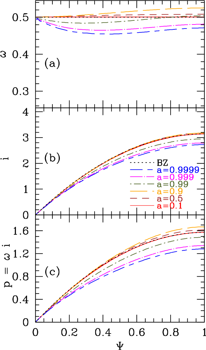
Figure 4.— Angular dependence of various quantities in a monopolar jet ($\nu=0$) as a function of the poloidal flux function $\Psi$. The different curves in each panel correspond to different values of the BH spin (see legend). From top to bottom the panels show the normalized field angular velocity $\omega=\Omega/\Omega_{\rm H}$, the normalized enclosed poloidal current $i=I/\Omega_{\rm H}$, and the normalized jet luminosity $p=\omega i=\Omega I/\Omega_{\rm H}^{2}=P/\Omega_{\rm H}^{2}$. The analytic BZ77 solution, shown with dotted lines, provides an excellent description of the numerical results for all spin values $a\lesssim 0.99$. Beyond this value of $a$, the quantities $\omega$, $i$, and $p$ all become noticeably smaller than the analytic solution. This trend is removed by the BZ6 solution (9), as shown in Figure 3.

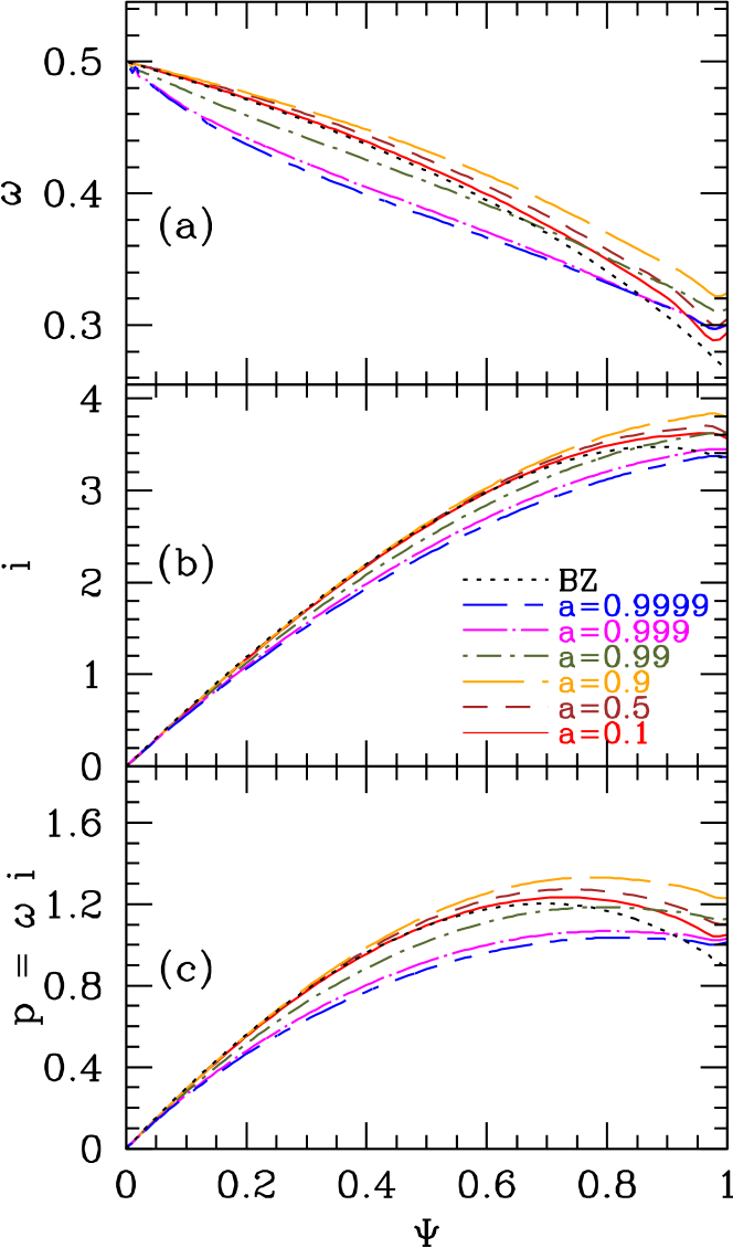
Figure 5.— Similar to Figure 4 but for a paraboloidal jet ($\nu=1,r_{0}=1$). Comparison with Figure 4 shows that, for the same BH spin, the angular velocity $\omega$ is smaller and the enclosed current $i$ larger in a paraboloidal jet compared to a monopolar jet. These two effects combine to give a smaller power output $p\equiv\omega{}i$ in the paraboloidal solution. Note that, whereas a monopolar jet rotates more or less like a rigid body, a paraboloidal jet has a significant variation of $\omega$ across its cross-section.

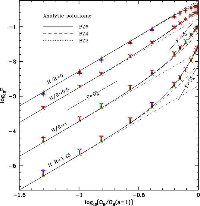
Figure 6.— Jet power output of various models as a function of dimensionless BH horizon spin frequency $\omega_{\rm H}=\Omega_{\rm H}/\Omega_{\rm H}(a=1)$ (see eq. 5) for four different choices of disk thickness: razor-thin disk with $H/R=0$, thicker disks with $H/R=0.5$, $1$, and $1.25$. For reference, the following values of BH spin, $a=\{0.2,0.5,0.9,1\}$, correspond to approximately the following values of $\omega_{\rm H}$: $\{0.1,0.27,0.63,1\}$. Numerical results for different models are shown with different symbols (see Fig. 3 caption for details). The second order analytic BZ2 solution is shown with dotted lines, the $4$th order BZ4 solution with dashed lines, and the $6$th order BZ6 solution with solid lines. As the disk becomes thicker, the spin dependence of jet power becomes steeper. This steepening is most accurately described by the BZ6 formula. Note that this formula also reproduces the flattening of the jet power for razor-thin disks ($H/R=0$) at high spins (Figure 3). For reference, we also show the slopes of various power-law scalings $P\propto\Omega_{\rm H}^{n}$ with straight line segments.

3.2. Power Output of Black Holes with Thick Disks

In all the models we described so far, the base of each polar jet covered a full $2\pi$ steradians at the BH horizon. However, observational evidence strongly suggests that low-luminosity BHs ($\lambda<0.01$, §1) are surrounded by thick accretion disks or ADAFs (Narayan & McClintock, 2008) with thicknesses $H/R\sim 1$. Here and below by the “disk thickness” $H/R$ we mean the angular extent at the BH horizon of the region exterior to the Poynting-dominated jet, i.e., the total thickness of the gaseous disk plus any magnetized corona or heavily mass-loaded wind above the disk. When a BH is surrounded by a thick disk/corona, equatorial field lines from the BH at lower latitudes pass through the disk/corona, become turbulent and produce a slow baryon-rich wind, whereas polar field lines at higher latitudes lie away from the disk gas and produce a Poynting-dominated relativistic jet (McKinney, 2005b). How does this effect modify the dependence of jet power on BH spin?

Assuming that both the total magnetic flux $\Phi_{\rm tot}$ threading the BH horizon and the angular thickness $H/R$ of the accretion disk/corona are independent of the BH spin, we can compute the power that is emitted in the Poynting-dominated region of the jet. We assume that the models we have described earlier continue to be valid, except that we integrate the jet power only over field lines that cross the horizon outside the $\pm H/R$ zone of the disk/corona. This procedure is well-motivated by general relativistic magnetohydrodynamical simulations of thick accretion disks which show that the relativistic jet subtends a well-defined solid angle for a given gas pressure scale height (McKinney & Gammie, 2004). We consider models with $H/R=0.5$, $1$, and $1.25$, and compare the results with the case of a razor-thin disk ($H/R=0$).

The results for the jet power as a function of disk thickness and spin are shown in Figure 6. As we have already seen, the jet power for a razor-thin disk scales as $P\propto\Omega_{\rm H}^{2}$ (this scaling is shown with dotted lines) until $a\lesssim 0.95$ after which it levels off. As the disk becomes thicker, the scaling changes qualitatively. For all thicknesses, $H/R=0.5$, $1$, and $1.25$, the power dependence on the spin follows the same $\Omega_{\rm H}^{2}$ power-law at low spins. However, at higher values of $a$, the power increases more steeply. The break occurs roughly at $a\sim 0.7$, with a moderate dependence on the disk thickness. Above the break for the case $H/R=1$ we have $P\propto\Omega_{\rm H}^{4}$ and for the case $H/R=1.25$ we have $P\propto\Omega_{\rm H}^{6}$. This steep dependence is similar to what was observed by McKinney (2005b) in his numerical simulations of turbulent accreting tori. We observe the same steep power dependence also in our ideal GRMHD simulations (§1).

We now explain the reason for the steep dependence of jet power on $\Omega_{\rm H}$ as $a\to 1$. We saw in Figures 1 and 2 that as the BH spin increases, magnetic field lines rearrange laterally and concentrate around the axis of rotation (see Komissarov & McKinney 2007 for an explanation of this effect in terms of hoop stresses). Figure 7 shows that this leads to a non-uniform distribution of radial magnetic field $B^{r}$ across the jet, with $B^{r}$ having a maximum near the rotation axis and a minimum near the jet boundary. Since the electromagnetic energy flux of a BH is proportional to $(B^{r})^{2}$ at the BH horizon (see equation A1), the concentration of magnetic flux near the rotation axis leads to a progressively larger fraction of the total energy output of the BH to be emitted in the polar region, giving a steeper dependence of jet power on the BH spin in the presence of a thick disk ($H/R\sim 1$). In a related context, MacDonald (1984) and Komissarov & McKinney (2007) have studied how magnetic flux is pulled in by a spinning BH by considering magnetic hoop stresses. MacDonald (1984) appears to have missed the strength of this effect by mostly investigating models with relatively small $a\lesssim 0.7$ and by primarily looking for a change in the total magnetic flux accumulated at the horizon rather than measuring the flux redistribution on the horizon.

We now describe an analytic approach for understanding the steep dependence of jet power on BH spin for thick disks with $H/R\sim 1$. While the split-monopolar magnetic field is an exact solution for non-spinning BHs, for spinning BHs the dragging of frames induces a spin-dependent perturbation to the split-monopolar magnetic field geometry. It is this perturbation that causes field lines to move preferentially toward the rotational axis. By performing an expansion in powers of $a$, BZ77 determined this perturbation of the magnetic field geometry to the lowest (second) order in BH spin $a$ (see also McKinney & Gammie 2004 and Tanabe & Nagataki 2008). Accounting for this perturbation in the field geometry, Tanabe & Nagataki (2008) determined the BH power output more accurately than the original BZ77 derivation, to the $4$th order in BH spin $a$. As we noted in §3.1, expansions in powers of BH frequency $\Omega_{\rm H}$ are more accurate at high spins than expansions in powers of the BH spin $a$. Therefore, in Appendix B we perform an equivalent expansion in terms of $\Omega_{\rm H}$. Figure 6 shows with dashed lines the power output of our $\Omega_{\rm H}$-based model, which we refer to as BZ4. Clearly, it provides a more accurate approximation for the power of our numerical jets than the $2$nd order accurate BZ2 solution shown with the dotted lines. However, as we saw in §3.1 and as is clear also from Figure 6, the BZ4 solution still does not capture a few important effects: (i) for BHs with razor-thin disks, it does not capture the flattening of the power output at $a\gtrsim 0.95$ and thereby over-predicts the numerical results by as much as $25$%, and (ii) for thick disks this solution under-predicts the numerical power by as much as $70$%.

To improve our analytic model, we have used the results of our numerical simulations to determine higher-order corrections to both the field geometry and the power of the BH at high spins. Firstly, we have obtained a higher-order accurate numerically-motivated expansion in powers of $\Omega_{\rm H}$ for the magnetic field $B^{r}$ at the BH horizon (Appendix C provides the details). Shown with dotted lines in Figure 7 for a wide range of $a$, this analytic approximation for $B^{r}$ accurately reproduces the numerical angular profile of magnetic field for a wide range of polar angles, $\theta_{\rm H}\gtrsim 0.3$ or $H/R\lesssim 1.3$. Secondly, based on this higher-order magnetic field profile, we have analytically computed the $6$th order accurate approximation for the BH power output, which we refer to as model BZ6 (see Appendix C for more detail). Figure 6 shows the results with the solid lines. Not only does the BZ6 expansion correctly capture the flattening of the BH power at high BH spins for razor-thin disks, it also provides a significantly more accurate approximation to the jet power output for thicker disks. For instance, for a thick disk with $H/R=1.25$, the BZ6 expansion is about a factor of $20$ more accurate than the BZ4 expansion.

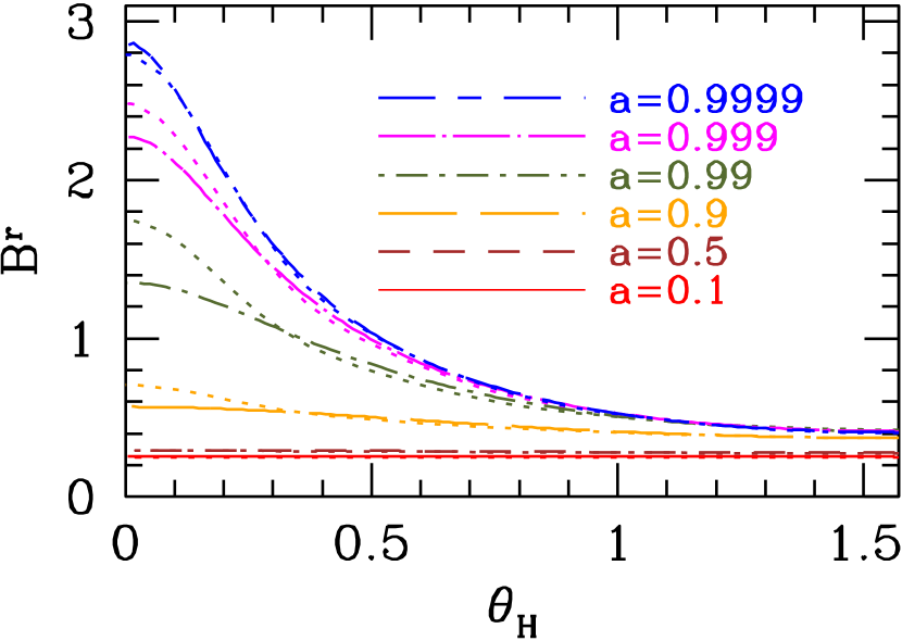
Figure 7.— Radial contravariant component of the magnetic field strength $B^{r}$ evaluated at the BH horizon in a monopolar model ($\nu=0,r_{0}=0$) as a function of polar angle $\theta_{\rm H}$, for different values of BH spin (see legend). As the spin of a BH is increased, magnetic field lines progressively bunch up toward the BH rotation axis, resulting in an increased magnetic field strength close to the axis at small $\theta_{\rm H}$ (this effect can also be seen in Figs. 1–2). Dotted colored lines show the high-order analytic solution, while the various other lines show the numerical solution (see legend).

4. Discussion

Figure 3 shows that, regardless of the geometry of the confining wall, the total power output of a magnetized relativistic spinning BH with a razor-thin disk varies as $P=k\Phi_{\rm tot}^{2}\Omega_{\rm H}^{2}$ (equation 7), where $\Phi_{\rm tot}$ is the total magnetic flux threading the BH horizon, $\Omega_{\rm H}=a/(2r_{\rm H})$ is the BH horizon frequency, and $r_{\rm H}=M\left[1+(1-a^{2})^{1/2}\right]$ is the radius of the BH horizon in units of $G/c^{2}$. This modified BZ2 scaling is slightly steeper than the original BZ77 scaling $P=k\Phi_{\rm tot}^{2}(a/4M)^{2}$ (equation 4). A more accurate BZ6 scaling (equation 9) accurately reproduces the power-spin dependence for all values of BH spin $a$, including the limit $a\to 1$.

In the context of the radio loud/quiet dichotomy of AGN, following Sikora et al. (2007) let us assume that supermassive BHs in elliptical galaxies, which manifest themselves as radio loud AGN, have higher spin parameters with a median $a\sim 0.9$, while the BHs in spirals, the radio quiet AGN, have a lower median $a\sim 0.3$ (e.g., Volonteri et al. 2007). Figure 3 then suggests that the jet powers in the two classes of objects (assuming similar values of $\Phi_{\rm tot}$) would differ by a factor $\sim 20$. However, radio loud AGN and radio quiet AGN differ in their radio luminosities by a factor $\sim 10^{3}$ (Sikora et al., 2007). What could be the reason for such a large dichotomy in jet power?

One motivation for the present study was to investigate whether there is any strong non-linearity in BH physics that might cause the jet power to increase very rapidly as the BH spin approaches unity. If this were the case, one could pursue a scenario in which radio loud AGN are associated with nearly extremal Kerr BHs. Unfortunately, our numerical results indicate that non-linearity hardly helps. Because the total BH power output scales as $\Omega_{\rm H}^{2}$ (equation 5) rather than simply as $a^{2}$, there is a slightly steeper increase of power with $a$ as the spin approaches unity. However, the scaling actually becomes shallower once $a$ increases above $\sim 0.99$. We have carefully checked the convergence of our models and we are confident that the results are not affected by numerical errors. Therefore, there is not much room for increasing the power of radio loud AGN jets by pushing $a$ arbitrarily close to unity.

Therefore, since there is not much wiggle room at the radio loud end, we need to postulate that radio quiet AGN have very low values of $a$, say $a\sim 0.03$. This is uncomfortably low. It is certainly feasible for an occasional BH to be spinning so slowly, but to have an entire population of BHs (radio quiet sources in spirals) with a median $a$ of order $0.03$ seems far-fetched. It would require spiral galaxies not to have experienced any significant mergers. Furthermore, the BHs in their nuclei should have accreted mass entirely through minor mergers with smaller companions, each with a tiny mass and with a random orientation of angular momentum (Hughes & Blandford, 2003; Gammie et al., 2004; Berti & Volonteri, 2008).

The second motivation for the present study was to investigate if the geometry of the confining funnel along which the jet propagates, which may be different for rapidly-spinning and slowly-spinning BHs, could lead to a substantial change in the jet power. This too turns out not to be the case, within the context of razor-thin disks. We have tried a wide range of geometries for the jet, as described in §2 (see also Figs. 1, 2), but the jet power varies by no more than $20\%$ for a fixed BH spin and magnetic flux.

Our third motivation was to investigate the correctness of the results of McKinney (2005b) who obtained a steeper dependence in the jet power compared to the total BH power. For this purpose, we considered in §3.2 an additional geometrical effect, viz., varying the solid angle subtended by the base of the jet. Such a variation is expected if the accretion disk is geometrically thick. As an example, let us consider the results corresponding to a BH surrounded by a disk of angular extent $H/R=1$, and let us further assume that radio loud AGN have spin parameters very close to unity and radio quiet AGN have more modest values of $a$. Then Figure 6 shows that it is possible to explain the radio loud/quiet dichotomy, i.e., a factor of $10^{3}$ in jet power, if radio loud AGN have $a\to 1$ and radio quiet systems have $a\sim 0.15$. This is a lot more comfortable than the requirement $a\sim 0.03$ that we found earlier for a razor-thin disk. Indeed, if the disk/corona is even thicker than $H/R\sim 1$, which is not unreasonable, the effect is even stronger (see Figure 6), and the radio loud/quiet dichotomy can be explained with quite modest changes in spin.

There are several other effects that we did not consider which might either enhance or diminish the effect of rapid spin. For instance, we assumed that the total magnetic flux threading the horizon is a constant, independent of BH spin. Any mechanism that enhances the total magnetic flux threading the horizon would lead to a larger BH power output (McKinney, 2005b; Hawley & Krolik, 2006; Komissarov & McKinney, 2007; Reynolds et al., 2006; Garofalo, 2009). For example, McKinney (2005b) found that the magnetic flux across the entire horizon scales as $\Phi_{\rm{}tot}\propto\Omega_{\rm H}^{1/2}$, so the total power will increase by another factor of $\Phi_{\rm{}tot}^{2}\propto\Omega_{\rm H}$, which further diminishes the range of BH spins required to explain the radio loud/quiet dichotomy. At first sight, it would appear that $\Phi_{\rm tot}$ is determined by conditions far from the BH, e.g., the net magnetic flux of the gas supplied to the accretion disk on the outside, and the ability of the disk gas to transport this field in. However, once the field has been transported to the center, two general relativistic effects kick in. First, the spin of the BH determines the size of the plunging region, and larger plunging regions can accumulate more flux (Garofalo, 2009). Note that magnetic flux can also be transported to the BH through the corona outside the accretion disk (Rothstein & Lovelace, 2008; Beckwith et al., 2009). Second, the frame-dragging of space-time near the BH within the ergospheric region leads to currents that generate hoop stresses pulling magnetic flux toward the horizon (Komissarov & McKinney, 2007). These two effects are non-trivially coupled, although for prograde BH spins the hoop stresses appear to dominate (McKinney, 2005b), while for retrograde BH spins the size of the plunging region may dominate (Garofalo, 2009). Another possibility is that a stronger dependence on spin could occur if some field lines attach between the disk and the BH (Ye & Wang, 2005), although such configurations are not seen in general relativistic magnetohydrodynamical simulations of accretion disks (Hirose et al., 2004; McKinney, 2005b).

Yet another possibility is that mass-loading of AGN jets might have a large effect on the jet power. For example, the BZ77 mechanism only operates at sufficiently high magnetization for a given BH spin. Thus, the magnetization and BH spin can together introduce a “magnetic switch” mechanism that can trigger powerful jet formation from the BH (Takahashi et al., 1990; Meier et al., 1997; Meier, 1999; Komissarov & Barkov, 2009). Another type of magnetic switch can be due to changes in the field geometry from dipolar to multipolar, which leads to significant mass-loading of the polar regions (McKinney & Gammie, 2004; Beckwith et al., 2008; McKinney & Blandford, 2009) and a factor of $\sim 10$ weaker total BH power output. The physics of jet mass-loading is presently uncertain, and this question needs to be investigated in more detail. Finally, changes in the disk thickness may also result in differences in the amount of magnetic flux accumulated or generated by turbulence near the BH (Meier, 2001).

Finally, we note that we have implicitly assumed in this paper that the radio luminosity of a jet is directly proportional to the total energy flux (Poynting and kinetic power) carried by the jet. Perhaps this is not the case. Any non-linearity in the mapping between radiative luminosity and jet power could have important consequences. In particular, we note that the interstellar medium (ISM) in a typical elliptical galaxy is very different from that in a typical spiral. Since the radio emission in a jet is produced when the jet interacts with the external ISM, this difference may well lead to a strong effect on the radio loudness of the jet.

In application to gamma-ray bursts (GRBs) and collapsars, an interesting question is whether they are powered by the BZ mechanism through an outflow from a central BH or by an outflow from an accretion disk. Komissarov & Barkov (2009) suggest that the BZ effect is operating in such a scenario (however, see Nagataki 2009).

5. Conclusions

We set out in this paper to explain the radio loud/quiet dichotomy of AGN in the context of the BH spin paradigm. For razor-thin disks, we found that BH spin alone is insufficient to explain the observations even if the radio loud and radio quiet populations have very different merger and accretion histories. However, we found that the presence of a thick disk, such as an ADAF, can significantly enhance the spin dependence of the power output, to the extent that it can reasonably account for the observed radio loud/quiet dichotomy. Our only modification to the revised spin paradigm of Sikora et al. (2007) is that both populations should contain a BH surrounded by a thick disk such that the jet subtends a small solid angle around the polar axis.

These results were obtained by performing general relativistic numerical simulations of collimated force-free and MHD jets from spinning magnetized BHs for a wide range of spins (up to $a=0.9999$) and jet confinement geometries. We showed that, regardless of the geometry, a BH threaded with a magnetic flux $\Phi_{\rm tot}$ and surrounded by a razor-thin disk produces a jet with power $P\approx k\Phi_{\rm tot}^{2}\Omega_{\rm H}^{2}$, where $k$ is a known constant factor which depends only weakly on the field geometry, $r_{\rm H}=M[1+(1-a^{2})^{1/2}]$ is the radius of the BH horizon, and $\Omega_{\rm H}=a/(2r_{\rm H})$ is the angular frequency of the BH. This result gives a somewhat steeper dependence of jet power on $a$ compared to the original scaling $P\propto a^{2}$ obtained by BZ77. Nevertheless, we conclude that for a fixed magnetic flux $\Phi_{\rm tot}$, even this revised scaling is much too shallow to explain the radio loud/quiet dichotomy of AGN. Our goal, therefore, was to identify any other effect that may cause the jet power to depend more steeply on BH spin.

We found that such an effect naturally exists. We showed that the power output of a BH surrounded by a thick accretion disk with $H/R\sim 1$ (this is the effective thickness of the disk, corona and mass-loaded disk wind), as expected in systems with advection-dominated accretion flows (ADAFs, Narayan & McClintock 2008), is $P\propto\Omega_{\rm H}^{4}$, and even $\propto\Omega_{\rm H}^{6}$ for very thick disks (§3.2). In this case we can explain the radio loud/quiet dichotomy by having two different populations of galaxies with modestly different BH spins. For the case $H/R=1$, the radio loud population needs to have large spins $a\simeq 1$ while the radio quiet AGN population needs to have $a\simeq 0.15$. Such spin values may plausibly result from differences in the merger and accretion histories of supermassive BHs in elliptical and spiral galaxies (§4).

We worked out in the Appendices a first principles analytic model which accurately reproduces our numerical results for the jet power over a wide range of BH spin and disk thickness (Figures 3, 6).

Appendix A Second-order–accurate Expansion of Black Hole Power

In this section we present a compact derivation of the BZ77 effect. We determine the power output of a spinning BH embedded into an externally-imposed split-monopolar magnetic field. This magnetic field is given by the flux function (2) with $\nu=0$ and $r_{0}=0$. The main difference of this derivation is that we perform it in the powers of the “natural” variable – the BH angular frequency $\Omega_{\rm H}$ that plays an important role in determining the BH power output. The power output density evaluated at the horizon of a spinning BH is (Blandford & Znajek 1977; McKinney & Gammie 2004)

$$F_{\rm E}(\theta)=\left[2(B^{r})^{2}\Omega(\Omega_{\rm H}-\Omega)rM\sin^{2}\theta\right]\Bigr{|}_{r=r_{\rm H}},$$ (A1)

where the quantity $\Omega$ is the angular frequency of magnetic field lines at the BH horizon and $B^{r}$ is the radial field strength at the horizon.

In order to determine the power output (A1), we need to know two quantities as functions of polar angle at the BH horizon: the radial magnetic field, $B^{r}$, and the field line angular frequency, $\Omega$. The element of the magnetic flux $d\Phi$ through the BH horizon is related to the radial magnetic field at the horizon through the following differential,

$$d\Phi=2\pi d\Psi=2\pi B^{r}\sqrt{-g}\,d\theta,$$ (A2)

where $g$ is the determinant of the Kerr metric in the Boyer-Lindquist coordinates, $\sqrt{-g}=(r^{2}+a^{2}\cos^{2}\theta)\sin\theta$. This formula closely resembles its cousin in the spherical polar coordinates and flat space where one has $\sqrt{-g}=r^{2}\sin\theta$. More generally, in place of $B^{r}$ we can use any vector field (e.g., energy flux), and the result is the differential of that flux. Assuming that the perturbations to the magnetic field away from a perfect split-monopole are higher order, we neglect them and obtain, by differencing the flux function (2) (with $\nu=0$ and $r_{0}=0$) according to (A2), an identical result to that in flat space:

$$B^{r}=\Psi_{\rm tot}/r^{2},$$ (A3)

where we neglected terms of order $\Omega_{\rm H}^{2}$ and higher. While the distribution of $\Omega$ needs to be self-consistently determined by solving the non-linear equations describing the balance of electromagnetic fields (we do so numerically in §3), here we make a simple yet accurate estimate based on the energy argument. Let us assume that the system chooses such a distribution of $\Omega$ that it causes an extremum in BH power output (A1). Such a value is clearly

$$\Omega=\Omega_{\rm H}/2$$ (A4)

since it maximizes the BH power output (A1) (see, e.g., Beskin & Kuznetsova, 2000). Despite the simplicity of this estimate, it is remarkably close to the true solution for the split-monopolar geometry as obtained from the numerical simulations (§3). Plugging equations (A3) and (A4) into the power output density (A1), we obtain

$$F_{\rm E}(\theta)=2\left(\Psi_{\rm tot}r^{-2}\right)^{2}(\Omega_{\rm H}/2)^{2}rM\sin^{2}\theta.$$ (A5)

Integrating up this power output density in angle in the same way as we integrated the magnetic field in equation (A2), we obtain the full power output into jets with an opening angle $\theta_{j}$:

$$P=2\times 2\pi\int_{0}^{\theta_{j}}F_{\rm E}(\theta)\sqrt{-g}\Bigr{|}_{r=r_{\rm H}}d\theta,$$ (A6)

where the extra factor of $2$ accounts for the fact that there are two jets, one in the northern and one in the southern hemisphere. Note that we are interested in an expansion of power up to 2nd order in $\Omega_{\rm H}$. Since the factor $F_{\rm E}(\theta)\propto\Omega_{\rm H}^{2}$ is already second order in $\Omega_{\rm H}$ (equation A5), we can without loss of accuracy evaluate the formula (A6) at $r=r_{\rm H}(a=0)=2M$ and replace $\sqrt{-g}$ with $\left[(2M)^{2}\sin\theta\right]$. After plugging into (A6) for $F_{\rm E}(\theta)$ using (A5) and evaluating the integral out to $\theta_{j}=\pi/2$, i.e., computing the full power output of the BH, we get:

$$P=\pi\Psi_{\rm tot}^{2}\Omega_{\rm H}^{2}\int_{0}^{\pi/2}\sin^{3}\theta\,d\theta=2\pi\Psi_{\rm tot}^{2}\Omega_{\rm H}^{2}/3,$$ (A7)

which is accurate to second order in $\Omega_{\rm H}$. In terms of the magnetic flux $\Phi_{\rm tot}=2\pi\Psi_{\rm tot}$, the formula becomes

$$P=k\Phi_{\rm tot}^{2}\Omega_{\rm H}^{2},$$ (A8)

with $k=1/(6\pi)$, which reproduces (7).

Appendix B Fourth-order–accurate Expansion of Black Hole Power

In Appendix A we have derived a second order accurate expression for power output of the BH in terms of the hole frequency $\Omega_{\rm H}$. The BH was embedded with a split-monopolar magnetic field. Let us now improve the accuracy of the previous derivation, this time retaining the higher order terms, up to $\Omega_{\rm H}^{4}$. A similar derivation was performed by Tanabe & Nagataki (2008) but in powers of BH spin $a$. Here we derive the expansion in terms of the natural variable $\Omega_{\rm H}$ which allows to use the expansion for nearly maximally spinning BHs. We also explicitly present the angular dependence of the BH power output.

In order to obtain a higher-order approximation to the power, this time we need to keep some of the higher terms we neglected in equations for $B^{r}$ (A3) and $\Omega$ (A4). Since $\Omega$ is an odd function of BH frequency, it contains only odd powers of $\Omega_{\rm H}$, therefore a higher order approximation for it has the following form:

$$\Omega={{}^{1}\!/_{2}}\Omega_{\rm H}+\mathcal{O}(\Omega_{\rm H}^{3}),$$ (B1)

where $\mathcal{O}(\Omega_{\rm H}^{3})$ denotes any third order or higher order terms in $\Omega_{\rm H}$. Since $P\propto\Omega_{\rm H}^{2}$, these higher-order terms contribute to the power output only terms of order higher than $\mathcal{O}(\Omega_{\rm H}^{4})$, therefore we neglect them. We do need, however, to include the terms that come from the higher order expansion of $B^{r}$. BZ77 showed that the dragging of frames by the spinning BH perturbs the magnetic field away from an exact split-monopole and have derived a second order correction to the flux function, $\Psi_{2}$, in powers of BH spin so that the full flux function has the form

$$\Psi(r,\theta) = \Psi_{0}(\theta)+a^{2}\Psi_{2}(r,\theta)+\mathcal{O}(a^{4})$$ (B2)

$$= \Psi_{0}(\theta)+16\Omega_{\rm H}^{2}\Psi_{2}(r,\theta)+\mathcal{O}(\Omega_{\rm H}^{4}),$$ (B3)

where we have used $a=4\Omega_{\rm H}+\mathcal{O}(\Omega_{\rm H}^{3})$. Here the zeroth and second order perturbations to the flux function are

$$\Psi_{0}(\theta)=1-\cos\theta,\quad\Psi_{2}(r,\theta)=f(r)\sin^{2}\theta\cos\theta,$$ (B4)

where $f(r)$ is a known function of radius $r$, but for further discussion only its value at the horizon of a non-spinning BH, $f(r=2)=\left(56-3\pi^{2}\right)/45$, is needed (this is because in the expansion (B3) we formally evaluate the coefficients at $\Omega_{\rm H}=0$, $r=r_{\rm H}=2$).

Combining expressions (B3), (B4) and (A2), we obtain the $2$nd-order–accurate radial magnetic field at the BH horizon:

$$B^{r}=\frac{\left(1+4{\Omega_{\rm H}}^{2}\right)^{2}\left[9+{\Omega_{\rm H}}^{2}(-49+6\pi^{2})(1+3\cos 2\theta)\right]}{9\left(r_{\rm H}^{2}\left(1+4{\Omega_{\rm H}}^{2}\right)^{2}+16{\Omega_{\rm H}}^{2}\cos\theta^{2}\right)}.$$ (B5)

Combining this expression with (A1), (A4) and plugging into (A6), we numerically obtain the angle-dependent enclosed power $P^{\rm BZ4}(\theta,\Omega_{\rm H})$ shown in Figure 6 as $P^{\rm BZ4}(\theta=\pi/2-H/R,\Omega_{\rm H})$ with dashed lines. This result, expanded to $4$th order in powers of $\Omega_{\rm H}$, is:

$$P^{\rm BZ4}(\theta,\Omega_{\rm H}) \approx \pi\Omega_{\rm H}^{2}\left[{{}^{4}\!/_{3}}\sin^{4}(\theta/2)(\cos\theta+2)\right]$$ (B6)

$$+ \pi\Omega_{\rm H}^{4}\bigl{[}90\left(3\pi^{2}-32\right)\cos\theta+\left(970-105\pi^{2}\right)\cos 3\theta+9\left(3\pi^{2}-26\right)\cos 5\theta+32\left(67-6\pi^{2}\right)\bigr{]}/{270}+\mathcal{O}(\Omega_{\rm H}^{6})$$

Clearly, at low spins, the second-order piece dominates, which we show in Figure 6 with dotted lines. However, at high spins, the fourth order piece can become dominant, which is confirmed in Figure 6. To see this more clearly, we perform an expansion of (B6) in powers of disk/corona thickness, $H/R\equiv\pi/2-\theta$, and obtain to second order in $H/R$:

$$P^{\rm BZ4}(H/R)\approx\Omega_{H}^{2}\left\{2.09-3.14H/R+\mathcal{O}[(H/R)^{3}]\right\}+\Omega_{H}^{4}\left\{2.9+1.7H/R+\mathcal{O}[(H/R)^{3}]\right\}+\mathcal{O}(\Omega_{\rm H}^{6}),$$ (B7)

where for clarity we have numerically evaluated the coefficients to two decimal places. This expansion makes it clear that as $H/R$ increases, the relative importance of the fourth order term increases. This also explains why in Figure 6 the $P\propto\Omega_{\rm H}^{4}$ dependence becomes more prominent for larger values of $H/R$ as opposed to smaller values.

Finally, we note that at the midplane the power output takes the following form (expanded up to $4$th order in $\Omega_{\rm H}$):

$$P^{\rm BZ4}(\theta=\pi/2)\approx{{}^{2\pi}\!/_{3}}\Psi_{\rm tot}^{2}\left[\Omega_{H}^{2}+\Omega_{H}^{4}\,8\left(67-6\pi^{2}\right)/45\right]+\mathcal{O}(\Omega_{\rm H}^{6})={{}^{2\pi}\!/_{3}}\Psi_{\rm tot}^{2}\left[\Omega_{H}^{2}+\alpha\Omega_{H}^{4}\right],$$ (B8)

where $\alpha=8\left(67-6\pi^{2}\right)/45\approx 1.38$. In this formula we have reintroduced $\Psi_{\rm tot}$ which was set to unity for the rest of this section. This result can also be expressed in terms of the total flux in the jet using $\Phi_{\rm tot}=2\pi\Psi_{\rm tot}$.

Appendix C Sixth-order–Accurate Expansion of Black Hole Power

Figure 6 shows that the fourth-order BZ4 solution for power is more accurate than the second-order solution. However, at high BH spin, $a\gtrsim 0.95$, it requires a more than a factor of $3$ correction in order to reproduce the numerical solution. Also, the fourth order BZ4 solution does not reproduce the flattening of the power dependence on the BH spin for razor-thin disks ($H/R=0$) at $a\gtrsim 0.95$.

Inspired by the success of the previous section, we would like to derive a sixth-order–accurate expression for the power. However, for that we would need to know the expansion of the flux function to the fourth order and of the field angular frequency to the third order. None of these are known analytically, therefore, we adopt a numerical approach.

Figure 4a shows the angular profiles of the field line rotation frequency $\Omega$ for different BH spins. While the deviations from the zeroth order approximation $\Omega=\Omega_{\rm H}/2$ are present, their relative magnitude is very small, $\lesssim 10$%. These $10$% changes in $\Omega/\Omega_{\rm H}$ translate into at most $1$% changes in the power output because the power depends quadratically on the magnitude of the higher order correction $(\Omega-\Omega_{\rm H}/2)$ (see equation 6). We are interested in the corrections of order $\sim 10{-}70$% (the level of inaccuracy of the BZ4 solution), therefore we neglect the higher-order corrections to $\Omega_{\rm H}$ in deriving the sixth order solution.

The corrections to the magnetic field shape are, however, dramatic. Figure 7 shows the angular distribution of the radial magnetic field $B^{r}$ at the BH horizon. As the BH spin increases, $B^{r}$ develops a progressively large non-uniformity in angle and deviates from the $4$th order solution by factors of a few. We therefore, attempt to find a numerical fit to the angular magnetic field dependence at the BH horizon for $a=0.9999$ by fitting to it the following trial function:

$$\Psi=\Psi_{0}+16\Omega_{\rm H}^{2}\Psi_{2}+\Omega_{\rm H}^{4}\Psi_{4},$$ (C1)

where the first two terms are given by equations (B4). We look for the spin-independent part of the third term, $\Psi_{4}$, in the following form

$$\Psi_{4}(\theta)=\sin^{2}(\theta)\left[c_{1}\cos^{\alpha_{1}}\theta+c_{2}\cos^{\alpha_{2}}\theta+c_{3}\cos^{\alpha_{3}}\theta+c_{4}\cos^{\alpha_{4}}\theta\right],$$ (C2)

where we choose $\alpha_{1}=25$, $\alpha_{2}=7$, $\alpha_{3}=3$, $\alpha_{4}=1$. In order to determine $4$ coefficients $c_{1}$–$c_{4}$, we match the numerical solution for $B^{r}$ at $a=0.9999$, shown in Figure 7, at $4$ angles: $\theta=0.1$, $0.5$, $0.7$, $\pi/2$. We find $c_{1}\approx 26.16$, $c_{2}\approx 22.72$, $c_{3}\approx 13.54$, $c_{4}\approx 2.08$. Figure 7 shows as dotted colored lines the solutions due to (C1) and (C2), with the above values of expansion coefficients, for various values of BH spin. Clearly, the analytic fit is a very good match to the power output at $\theta_{\rm H}\gtrsim 0.3$. Very close to the rotation axis, however, (at angles smaller than $0.3$) the fourth-order–accurate solution to the flux function (C1) is not enough: while we have a nearly perfect match between our fit and the numeric solution for $B6$ at high ($a=0.9999$) and mid-range ($a=0.5$) spins, our fit to $B^{r}$ deviates by up to $\sim 25$% at the in-between spins ($a\simeq 0.9{-}0.99$). However, the total power emitted into the range of polar angles $\theta\lesssim 0.3$ is very small, therefore these deviations of our fit from the numerical solution hardly influence the fit to the power output.

We also considered a direct fit to the vector spherical harmonic functions that form a complete set for the vector potential as given by equation B8 in McKinney & Narayan (2007a). However, even an expansion up to $l=10$ did not fit the very steep behavior of $B^{r}$ near the polar axis. However, otherwise, even only using up to $l=6$ does a reasonable job at fitting the numerical solution for the total power vs. spin and angle. This fact and the fact that a power of $25$ for $\cos\theta$ was required to fit the numerical results demonstrates that the numerical solution at $a\sim 1$ is highly non-linear with respect to $\theta$ and would be quite difficult to derive analytically. This proves the usefulness of the numerical simulations.

Now we are in a position to analytically compute the high-order–accurate power of our jets. Using (A2), we compute the radial field on the horizon, $B^{r}$, from the fourth-order flux function (C1). We then insert this field and the field angular frequency $\Omega$ (A4) into formula (A6) and obtain the angular-dependent jet power. This power, which we refer to as the sixth-order analytic BZ6 solution, is shown in Figure 6 with solid lines for various disk thicknesses and spins. (We compute these lines by numerically integrating the analytically-determined power in our jets. We note while formally this solution is $6$th order-accurate, its expansion in powers of $\Omega_{\rm H}$ contains important terms up to $10$th order. This highlights the non-linearity of the problem.) Clearly, these lines approximate the numerical data points very well, within $20$% for the whole range of disk thicknesses and spins that we have explored. Over most of the parameter space the errors are smaller than this value (they are largest for the thicker disks with $H/R\gtrsim 1.25$ that have the BH spin in the range $0.8\lesssim a\lesssim 0.99$).

References

- Allen et al. (2006) Allen, S. W., Dunn, R. J. H., Fabian, A. C., Taylor, G. B., & Reynolds, C. S. 2006, MNRAS, 372, 21
- Baum et al. (1995) Baum, S. A., Zirbel, E. L., & O’Dea, C. P. 1995, ApJ, 451, 88
- Beckwith et al. (2008) Beckwith, K., Hawley, J. F., & Krolik, J. H. 2008, ApJ, 678, 1180
- Beckwith et al. (2009) —. 2009, ApJ, 707, 428
- Begelman et al. (1984) Begelman, M. C., Blandford, R. D., & Rees, M. J. 1984, Reviews of Modern Physics, 56, 255
- Begelman & Li (1994) Begelman, M. C. & Li, Z.-Y. 1994, ApJ, 426, 269
- Benson & Babul (2009) Benson, A. J. & Babul, A. 2009, MNRAS, 397, 1302
- Berti & Volonteri (2008) Berti, E. & Volonteri, M. 2008, ApJ, 684, 822
- Beskin (2009) Beskin, V. S. 2009, MHD Flows in Compact Astrophysical Objects: Accretion, Winds and Jets (Springer)
- Beskin & Kuznetsova (2000) Beskin, V. S. & Kuznetsova, I. V. 2000, Nuovo Cimento B Serie, 115, 795
- Blandford (1990) Blandford, R. D. 1990, in Active Galactic Nuclei, ed. T. J.-L. Courvoisier & M. Mayor, 161–275
- Blandford (1999) Blandford, R. D. 1999, in Astronomical Society of the Pacific Conference Series, Vol. 160, Astrophysical Discs - an EC Summer School, ed. J. A. Sellwood & J. Goodman, 265
- Blandford & Rees (1974) Blandford, R. D. & Rees, M. J. 1974, MNRAS, 169, 395
- Blandford & Rees (1992) Blandford, R. D. & Rees, M. J. 1992, in American Institute of Physics Conference Series, Vol. 254, American Institute of Physics Conference Series, ed. S. S. Holt, S. G. Neff, & C. M. Urry, 3–19
- Blandford & Znajek (1977) Blandford, R. D. & Znajek, R. L. 1977, MNRAS, 179, 433
- Blundell (2008) Blundell, K. M. 2008, in Astronomical Society of the Pacific Conference Series, Vol. 386, Extragalactic Jets: Theory and Observation from Radio to Gamma Ray, ed. T. A. Rector & D. S. De Young, 467
- Catlett et al. (2007) Catlett, C., Andrews, P., Bair, R., et al. 2007, HPC and Grids in Action, Amsterdam
- Fender et al. (2004) Fender, R. P., Belloni, T. M., & Gallo, E. 2004, MNRAS, 355, 1105
- Gammie et al. (2003) Gammie, C. F., McKinney, J. C., & Tóth, G. 2003, ApJ, 589, 444
- Gammie et al. (2004) Gammie, C. F., Shapiro, S. L., & McKinney, J. C. 2004, ApJ, 602, 312
- Garofalo (2009) Garofalo, D. 2009, ApJ, 699, 400
- Ghosh & Abramowicz (1997) Ghosh, P. & Abramowicz, M. A. 1997, MNRAS, 292, 887
- Hawley & Krolik (2006) Hawley, J. F. & Krolik, J. H. 2006, ApJ, 641, 103
- Hirose et al. (2004) Hirose, S., Krolik, J. H., De Villiers, J.-P., & Hawley, J. F. 2004, ApJ, 606, 1083
- Ho et al. (2000) Ho, L. C. et al. 2000, ApJ, 541, 120
- Hughes & Blandford (2003) Hughes, S. A. & Blandford, R. D. 2003, ApJ, 585, L101
- Ivezić et al. (2004) Ivezić, Z., Lupton, R., Johnston, D., Richards, G., Hall, P., Schlegel, D., Fan, X., Munn, J., Yanny, B., Strauss, M., Knapp, G., Gunn, J., & Schneider, D. 2004, in Astronomical Society of the Pacific Conference Series, Vol. 311, AGN Physics with the Sloan Digital Sky Survey, ed. G. T. Richards & P. B. Hall, 437
- Jorstad et al. (2005) Jorstad, S. G., Marscher, A. P., Lister, M. L., Stirling, A. M., Cawthorne, T. V., Gear, W. K., Gómez, J. L., Stevens, J. A., Smith, P. S., Forster, J. R., & Robson, E. I. 2005, AJ, 130, 1418
- Kellermann et al. (1989) Kellermann, K. I., Sramek, R., Schmidt, M., Shaffer, D. B., & Green, R. 1989, AJ, 98, 1195
- Komissarov (2001) Komissarov, S. S. 2001, MNRAS, 326, L41
- Komissarov & Barkov (2009) Komissarov, S. S. & Barkov, M. V. 2009, MNRAS, 397, 1153
- Komissarov et al. (2007) Komissarov, S. S., Barkov, M. V., Vlahakis, N., & Königl, A. 2007, MNRAS, 380, 51
- Komissarov & McKinney (2007) Komissarov, S. S. & McKinney, J. C. 2007, MNRAS, 377, L49
- Komissarov et al. (2009) Komissarov, S. S., Vlahakis, N., Königl, A., & Barkov, M. V. 2009, MNRAS, 394, 1182
- Livio et al. (1999) Livio, M., Ogilvie, G. I., & Pringle, J. E. 1999, ApJ, 512, 100
- MacDonald (1984) MacDonald, D. A. 1984, MNRAS, 211, 313
- McKinney (2005a) McKinney, J. C. 2005a, astro-ph/0506368
- McKinney (2005b) —. 2005b, ApJ, 630, L5
- McKinney (2006a) —. 2006a, MNRAS, 367, 1797
- McKinney (2006b) —. 2006b, MNRAS, 368, 1561
- McKinney & Blandford (2009) McKinney, J. C. & Blandford, R. D. 2009, MNRAS, 394, L126
- McKinney & Gammie (2004) McKinney, J. C. & Gammie, C. F. 2004, ApJ, 611, 977
- McKinney & Narayan (2007a) McKinney, J. C. & Narayan, R. 2007a, MNRAS, 375, 513
- McKinney & Narayan (2007b) —. 2007b, MNRAS, 375, 531
- Meier (1999) Meier, D. L. 1999, ApJ, 522, 753
- Meier (2001) —. 2001, ApJ, 548, L9
- Meier (2002) —. 2002, New Astronomy Review, 46, 247
- Meier et al. (1997) Meier, D. L., Edgington, S., Godon, P., Payne, D. G., & Lind, K. R. 1997, Nature, 388, 350
- Mignone & McKinney (2007) Mignone, A. & McKinney, J. C. 2007, MNRAS, 378, 1118
- Moderski et al. (1998) Moderski, R., Sikora, M., & Lasota, J. 1998, MNRAS, 301, 142
- Nagataki (2009) Nagataki, S. 2009, ApJ, 704, 937
- Narayan & McClintock (2008) Narayan, R. & McClintock, J. E. 2008, New Astronomy Review, 51, 733
- Nemmen et al. (2007) Nemmen, R. S., Bower, R. G., Babul, A., & Storchi-Bergmann, T. 2007, MNRAS, 377, 1652
- Noble et al. (2006) Noble, S. C., Gammie, C. F., McKinney, J. C., & Del Zanna, L. 2006, ApJ, 641, 626
- Phinney (1983) Phinney, E. S. 1983, Ph.D. Thesis
- Reynolds et al. (2006) Reynolds, C. S., Garofalo, D., & Begelman, M. C. 2006, ApJ, 651, 1023
- Rothstein & Lovelace (2008) Rothstein, D. M. & Lovelace, R. V. E. 2008, ApJ, 677, 1221
- Sikora et al. (2007) Sikora, M., Stawarz, Ł., & Lasota, J.-P. 2007, ApJ, 658, 815
- Steenbrugge & Blundell (2008) Steenbrugge, K. C. & Blundell, K. M. 2008, MNRAS, 388, 1457
- Steenbrugge et al. (2008) Steenbrugge, K. C., Blundell, K. M., & Duffy, P. 2008, MNRAS, 388, 1465
- Steenbrugge et al. (2010) Steenbrugge, K. C., Heywood, I., & Blundell, K. M. 2010, MNRAS, 401, 67
- Takahashi et al. (1990) Takahashi, M., Nitta, S., Tatematsu, Y., & Tomimatsu, A. 1990, ApJ, 363, 206
- Tanabe & Nagataki (2008) Tanabe, K. & Nagataki, S. 2008, Phys. Rev. D, 78, 024004
- Tchekhovskoy et al. (2007) Tchekhovskoy, A., McKinney, J. C., & Narayan, R. 2007, MNRAS, 379, 469
- Tchekhovskoy et al. (2008) —. 2008, MNRAS, 388, 551
- Tchekhovskoy et al. (2009a) —. 2009a, ApJ, 699, 1789
- Tchekhovskoy et al. (2009b) Tchekhovskoy, A., Narayan, R., & McKinney, J. C. 2009b, ArXiv:0909.0011 (astro-ph)
- Volonteri et al. (2007) Volonteri, M., Sikora, M., & Lasota, J.-P. 2007, ApJ, 667, 704
- Wilson & Colbert (1995) Wilson, A. S. & Colbert, E. J. M. 1995, ApJ, 438, 62
- Ye & Wang (2005) Ye, Y. & Wang, D. 2005, MNRAS, 357, 1155