Black holes and Galactic density cusps – I. Radial orbit cusps and bulges

Abstract

In this paper, we study the distribution functions that arise naturally during self-similar radial infall of collisionless matter. Such matter may be thought of either as stars or as dark matter particles. If a rigorous steady state is assumed, then the system is infinite and is described by a universal distribution function given the self-similar index. The steady logarithmic potential case is exceptional and yields the familiar Gaussian for an infinite system with an inverse-square density profile. We show subsequently that for time-dependent radial self-similar infall, the logarithmic case is accurately described by the Fridmann and Polyachenko distribution function. The system in this case is finite but growing. We are able to embed a central mass in the universal steady distribution only by iteration, except in the case of massless particles. The iteration yields logarithmic corrections to the massless particle case and requires a ‘renormalization’ of the central mass. A central spherical mass may be accurately embedded in the Fridmann and Polyachenko growing distribution however. Some speculation is given concerning the importance of radial collisionless infall in actual galaxy formation.

1 Introduction

The relation between the formation of black holes and of galaxies has developed into a key astrophysical question, from the early papers by Kormendy and Richstone [Kormendy & Richstone 1995], to the more recent discoveries by Magorrian et al. [Magorrian et al. 1998], Ferrarese and Merritt [Ferrase & Merritt 2000], and Gebhardt et al.[Gebhardt et al., 2000]. Recent papers [Graham 2004, Kormendy & Bender 2009] also establish a correlation between black hole mass and bulge luminosity deficit. These papers establish a strong correlation between what is essentially the black hole mass and the surrounding stellar bulge mass (or velocity dispersion). The origin of this proportionality, which extends well beyond the gravitational dominance of the black hole, remains uncertain. But it is generally taken to imply a coeval growth of the black hole and bulge.

Various proposals have been offered to explain the black hole mass-bulge mass proportionality as a consequence of the AGN phase. There is as yet no generally accepted scenario although a kind of ‘auto-levitation’, based on radiative feed-back from the accreting black hole to the star-forming gas that in turns limit accretion, is plausible. In any event there remains the question of the origin of the black hole seed masses. In some galaxies at very high red shift the inferred black hole masses are already of order $10^{9}\leavevmode\nobreak\ M_{\odot}$ [Kurk et al., 2007, e.g.] after about one Ga of cosmic time. This may require frequent, extremely luminous early events [Walter et al., 2009, e.g.], or it may suggest an alternate growth mechanism.

The latter possibility is reinforced by the detection of a change in the normalization of the black hole mass-bulge mass proportionality in the sense of relatively larger black holes at high red shift [Maiolino et al. 2007, e.g.]. As suggested in that paper it seems that the black holes may grow first, independently of the bulge. The collisionless matter that we invoke might be stars or it might be the dark matter itself.

Recently [Peirani & de Freitas Pacheco 2008] have studied the possible size of the dark matter component in black hole masses. By assuming that the dimensional or ’pseudo-phase-space density’ [H2006, i.e. Henriksen 2006b, e.g.] is strictly constant they convert the relativistic accretion of the dark matter into an adiabatic Bondi flow problem and obtain the resulting accretion rate. Then by adopting the mass proportionality between bulge and black hole and fitting boundary conditions from cosmological halo simulations, they deduce that between 1% and 10% of the black hole mass could be due to dark matter.

If we accept this result at face value, a seed mass of say $10^{6}M_{\odot}$ could have grown from dark matter. It would now be part of a super massive black hole that subsequently grew in the AGN phase. Some seeds may be primordial. As early as 1978, through fully general relativistic numerical collapse calculations, [Bicknell & Henriksen 1979] predicted primordial black hole masses in the range $10^{2}$ to $10^{6}M_{\odot}$.

Stellar density cusps surrounding black holes have been studied extensively previously. Classic studies by [Peebles 1972] and by [Bahcall & Wolf 1976] dealt with the problem of feeding the black hole from a filled loss cone (nearly radial orbits). In addition to these diffusion studies, Young [Young 1980] explored the cusps produced by the adiabatic growth of a black hole in a pre-existing isothermal stellar environment. This was extended by [Quinlan et al 1995] and by [MacMillan & Henriksen 2002] to more general environments. In a cosmological context, Bertschinger [1985] also studied the growth of a central black hole by radial infall. The conclusions were that the black hole induced cusps were never flatter than $r^{-1.5}$ (the isothermal and cosmological case) and that no black hole mass-bulge mass correlation was established [MacMillan & Henriksen 2002]. The latter conclusion has spurred the investigation of coeval dynamical growth of the black hole and bulge in contrast to adiabatic growth [MacMillan & Henriksen 2003]. In this paper we discuss possible coeval growth due to radial infall of stars and dark matter that both feed the black hole and establish a collisionless cusp with a self-similar distribution function.

In this and subsequent papers [I, II, III] we will embed a black hole (or at least a central mass) in a distribution of particles that arises naturally during the formation of the galactic core. The ‘natural evolution’ is taken to be that of self-similarity since power-law behaviour is observed both in reality and in simulations. In this fashion we introduce some uniqueness into the form of the resulting distribution function that describes the collisionless matter that surrounds the central mass. We will predict the consequent density cusp profile and that of the velocity dispersion variation in the cusp.

In this first paper we confine ourselves to radial infall. The first general result on radial infall was in fact given in [Fillmore & Goldreich, 1984] and the Bertschinger [1985] result follows by putting their parameter $\epsilon_{FG}=1/3$. However neither this work nor that of Bertschinger attempted to infer closed forms for the equilibrium distribution function. This was begun by Henriksen & Widrow (1995) (hereinafter [HW95]). In [H2006] it is pointed out that $a=9/8$ ($\epsilon=3$) yields the Bertschinger solution in its entirety, including the recently heralded power law of the proxy for phase space density. The parameter $\epsilon=3\epsilon_{FG}$ and it is related to the index called ‘$a$’ below, both by simulations and theory.

We deduce in this paper two principal distribution functions that arise naturally. One is steady and infinite and can not contain a central mass exactly. However we can treat the central mass as a perturbation to the gravitational field and iterate on the Boltzmann and Poisson equations to find the flattest possible cusp in a steady infinite system surrounding a central mass. There is a special logarithmic case in this category that yields a Gaussian distribution function and an inverse square law density cusp. Our derivation is new but the result agrees with the form deduced in [Lynden-Bell 1967] based on statistical mechanics.

Our second result is most important in that it represents a growing cusp wherein a central mass may be embedded exactly. It is the Fridmann and Polyachenko distribution function, which has not previously been identified in this physical context. We derive it theoretically and verify it with simulations. It also corresponds to a logarithmic potential for which the self-similar index $a$ (see below) is unity. The compatibility with a central mass allows us to give a growth rate for that mass. It is perhaps significant in light of the extensive orbital study of [Van den Bosch et al. 2008] that we are most successful with our embedding in a time dependent case. For these authors suggest that the central mass may render the orbits chaotic and nonstationary.

We are aware that such a radial system is unstable to the radial orbit instability (ROI) on small scales [MWH 2006, hereinafter for MacMillan et al. 2006]. However even fully cosmological simulations show an outer envelope wherein the orbits are trending to be radial. Moreover isolated halos, which also show statistical relaxation that is begging to be understood, show quite radial orbits in the envelope [MWH 2006]. In such cases the ‘central mass’ may be a central ‘bulge’ of dark matter that forms rapidly. We speculate below that the growth of this bulge in such an envelope may be described in terms of radial infall, and that this infall may continue hierarchically to smaller scales after relaxation by the ROI and clump-clump interactions [MacMillan & Henriksen 2003]. Such interactions would remove angular momentum from some particles in favour of others and so create the continuing radial infall.

We begin the next section with the general formulation in spherical symmetry. Subsequently in section 3 we discuss the various possible rigorously steady distribution functions (DF from now on) for radial orbits. We show in section 4 that the DF of Fridman and Polyachenko [Fridmann & Polyachenko 1984, hereafter called FPDF] describes a system of radial orbits that is growing self-similarly. This is contrasted in the same section with an infinite steady system for which the DF is Gaussian. After some discussion, we give our conclusions.

2 Dynamical Equations in Infall Variables

Following the formulation of [H2006] in this section we transform the collisionless Boltzmann and Poisson equations to ‘infall variables’. We treat a spherically symmetric anisotropic system in the ‘Fujiwara’ form [Fujiwara 1983, e.g.] namely

$$\frac{\partial f}{\partial t}+v_{r}\frac{\partial f}{\partial r}+\left(\frac{j^{2}}{r^{3}}-\frac{\partial\Phi}{\partial r}\right)\frac{\partial f}{\partial v_{r}}=0,$$ (1)

$$\frac{\partial}{\partial r}\left(r^{2}\frac{\partial\Phi}{\partial r}\right)=4\pi^{2}G\int f(r,v_{r},j^{2})dv_{r}dj^{2},$$ (2)

where $f$ is the phase-space mass density, $\Phi$ is the ‘mean’ field gravitational potential, $j^{2}$ is the square of the specific angular momentum and other notation is more or less standard.

The ‘infall variables’ are a system of variables and coordinates that allows us either to readily take the self-similar limit or to retain a memory of previous self-similar dynamical relaxation into a true steady state. In this way we can remain ‘close’ to self-similarity just as the simulations appear to do. These coordinates [Henriksen 2006a, H2006] allow the general expression of the Vlasov-Poisson set, but they also contain a parameter ($a$) that reflects underlying self-similarity. The self-similar limit is taken by assuming what we term ‘self-similar virialisation’, wherein the system is steady in these coordinates, although it is not absolutely steady since mass is accumulating in this mode.

The transformation to infall variables has the form [H2006, e.g.]

$$R =r\,e^{-\alpha T/a},\hskip 56.9055ptY=v_{r}e^{-(1/a-1)\alpha T},$$

$$Z =j^{2}e^{-(4/a-2)\alpha T},\hskip 27.03003pte^{\alpha T}=\alpha t,$$

$$P\left(R,Y,Z;T\right) =e^{(3/a-1)\alpha T}\pi f\left(r,v_{r},j^{2};t\right),$$ (3)

$$\Psi\left(R;T\right) =e^{-2(1/a-1)\alpha T}\Phi(r),$$

$$\Theta\left(R;T\right) =\rho(r,t)e^{2\alpha T}.$$

This transformation is inspired by the nature of self-similarity, which can be understood as a scaling group wherein each quantity scales according to its dimensions [Carter & Henriksen,1991]. The group parameter is the logarithmic time $T$. The combinations of scaling constants (note that $a\equiv\alpha/\delta$ see below) multiplying $\alpha T$ in the exponential factor of each physical quantity reflect the dimensions of that quantity. When the dependence on the parameter $T$ is retained in the new variables, there is clearly no invariance along the scaling group motion and so no self-similarity. This means that the passage to the self-similar limit requires taking $\partial_{T}=0$ when acting on the transformed variables. Thus the self-similar limit is a stationary system in these variables, which is a state that we have described elsewhere as ‘self-similar virialisation’ [HW 1999, Le Delliou 2001, i.e. Henriksen & Widrow 1999]. The virial ratio $2K/|W|$ is a constant in this state (although greater than one; $K$ is kinetic energy and $W$ is potential), but the system is not steady in physical, i.e. untransformed, variables, since infall continues.

The single constant quantity $a$ is the constant that determines the dynamical similarity, called the self-similar index. It is composed of two separate scalings, $\alpha$ in time and $\delta$ in space, in the form $a\equiv\alpha/\delta$. The dimensions of any mechanical quantity can be expressed in the scaling space $\boldsymbol{a}\equiv(\alpha,\delta,\mu)$, where $\mu$ is the mass scaling. The exponential factor of any physical quantity $Q$ (which includes physical constants) is calculated as $\boldsymbol{a}\cdot\boldsymbol{d}_{Q}$ where $\boldsymbol{d}_{Q}$ describes the quantity $Q$ in scaling space. Thus for the velocity $\boldsymbol{d}_{v}=(-1,1,0)$, for the distribution function $\boldsymbol{d}_{f}=(3,-6,1)$ and for Newton’s constant $\boldsymbol{d}_{G}=(-2,3,-1)$. In a gravitation problem the scalings $\alpha$ and $\delta$ can express the scalings of all physical quantities having mass, length and time dimensions. This is because we require $G$ to be constant under the scaling motion so that $\boldsymbol{a}\cdot\boldsymbol{d}_{G}=0$ and hence $\mu=3\delta-2\alpha$. This changes $\boldsymbol{d}_{f}$ to $(1,-3)$ as used in equation (3). This procedure yields the constants in the exponential factors transforming all physical quantities in the equations (3).

We assume that time, radius, velocity and density are measured in fiducial units $r_{o}/v_{o}$,$r_{o}$, $v_{o}$ and $\rho_{o}$ respectively. The unit of the distribution function is $f_{o}$ and that of the potential is $v_{o}^{2}$. We remove constants from the transformed equations by taking

$$f_{o}=\rho_{o}/v_{o}^{3},\leavevmode\nobreak\ \leavevmode\nobreak\ \leavevmode\nobreak\ \leavevmode\nobreak\ \leavevmode\nobreak\ \leavevmode\nobreak\ v_{o}^{2}=4\pi G\rho_{o}r_{o}^{2}.$$ (4)

These transformations convert equations (1),(2) to the respective forms

$$\frac{1}{\alpha}\partial_{T}P-\left(\frac{3}{a}-1\right)P+(\frac{Y}{\alpha}-\frac{R}{a})\partial_{R}P\\ -\left[\left(\frac{1}{a}-1\right)Y+\frac{1}{\alpha}\left(\frac{\partial\Psi}{\partial R}-\frac{Z}{R^{3}}\right)\right]\partial_{Y}P-\left(\frac{4}{a}-2\right)Z\partial_{Z}P=0$$ (5)

and

$$\frac{1}{R^{2}}\frac{\partial}{\partial R}\left(R^{2}\frac{\partial\Psi}{\partial R}\right)=\Theta.$$ (6)

This integro-differential system is closed by

$$\Theta=\frac{1}{R^{2}}\int\leavevmode\nobreak\ PdY\leavevmode\nobreak\ dZ.$$ (7)

Until we enforce the self-similar limit ($\partial/\partial T=0$) these equations remain completely general, because we have made a continuous and invertible change of variables in equation (3). The merit of the transformation at this stage is only that it puts the expected asymptotic self-similar behaviour in the explicit exponential factors, while relegating the declining time dependence leading to this state to the transformed variables. These variables are strictly independent of $T$ in the self-similar state.

We will in this paper restrict ourselves to the filled loss cone limit of radial infall [HLeD 2002], although this is not the case in subsequent papers of this series. This special case is certainly not realistic where angular momentum becomes important, but it may have application on large scales and in the subsequent evolution in regions where angular momentum is transformed away either by bars or other asymmetries. It may in any case be regarded as an introduction to our methods.

To proceed we set

$$P=F(R,Y;T)\delta(Z)=F(R,Y;T)\delta(j^{2})(e^{(4/a-2)\alpha T})$$

($\delta()$ is the Dirac delta, not the scaling delta) which changes the scaling for the DF in equation (3) to

$$\pi f=F(R,Y,;T)e^{(1/a-1)\alpha T}\leavevmode\nobreak\ \delta(j^{2}),$$ (8)

while other scalings remain unchanged.

The governing equations now become equation (6) plus the Boltzmann equation for $F(R,Y;T)$ in the form

$$\frac{1}{\alpha}\partial_{T}F+\left(\frac{1}{a}-1\right)F+\left(\frac{Y}{\alpha}-\frac{R}{a}\right)\partial_{R}F\\ -\left[\left(\frac{1}{a}-1\right)Y+\frac{1}{\alpha}\frac{\partial\Psi}{\partial R}\right]\partial_{Y}F=0.$$ (9)

Finally equation (7) reduces to

$$\Theta=\frac{1}{R^{2}}\leavevmode\nobreak\ \int\leavevmode\nobreak\ F\leavevmode\nobreak\ dY.$$ (10)

This completes the formalism that we will use to obtain the results below.

3 Steady Cusps and Bulges with Radial Orbits

In this section, we find DFs both self-similar and steady which are comprised of collisionless particles in radial orbits. We expect one mode of relaxation in collisionless cusps to be of the ‘moderately violent’ type satisfying, in terms of the particle energy $E$ and mean field potential $\Phi$, the relation

$$\frac{\mathrm{d}E}{\mathrm{d}t}=\frac{\partial\Phi}{\partial t}|_{r}.$$ (11)

This includes phase-mixing. Another mode [Diemand et al., 2006] is furnished by the presence of hierarchical sub-structure . The sub-structure can interact in clump-clump interactions that can induce relaxation on a coarse-grained scale [H2009, i.e. Henriksen 2009].

However the temporal evolution of the system is difficult to follow analytically even in the self-similar limit, so we normally look for equilibria established by the evolution.This may be either a strictly steady state in some appropriate coarse-grained description, or it may be a self-similar virialised state.

In general one can not find a unique solution of the governing equations that consistently reproduce infall onto a central mass. We find that this is possible in one interesting case (Fridman and Polyachenko DF) of accretion onto a point mass that arises naturally, but not for a truly steady distribution around a point mass. One can allow for the presence of a point mass in a rigorously steady distribution by iterating about an equilibrium state that is determined initially by the central mass. This allows the central mass and the environment to be evolved together towards a new equilibrium, although normally only a single loop is feasible (we give two loops below as a confirmation of the continuing logarithmic behaviour). We proceed to derive these two results in this section.

Using the characteristics of equation (9) plus the total derivative

$$\frac{\mathrm{d}\Psi}{\mathrm{d}s}=\frac{\partial\Psi}{\partial s}+\frac{\mathrm{d}R}{\mathrm{d}s}\partial_{R}\Psi$$ (12)

where $\mathrm{d}s\equiv\alpha\mathrm{d}T$, one finds by a simple manipulation that

$$\frac{\mathrm{d}\left(\frac{Y^{2}}{2}+\Psi\right)}{\mathrm{d}s}=-2\left(\frac{1}{a}-1\right)\frac{Y^{2}}{2}-\frac{R}{a}\partial_{R}\Psi+\frac{\partial\Psi}{\partial s}.$$ (13)

In order for this last equation to yield the energy as an isolating integral (i.e. characteristic constant), the sum of the last two terms must give $-2(1/a-1)\Psi$. This is most simply effected by setting $\partial\Psi/\partial s=0$ and $R\partial_{R}\Psi=p\Psi$, which turns out to be a condition for both self-similarity and a true steady state. Here

$$p=2(1-a).$$ (14)

so that $\Psi=\Psi_{o}R^{p}$ for some constant $\Psi_{o}$.

Hence, on setting $\mathcal{E}\equiv Y^{2}/2+\Psi$, we have from equation (13)

$$\frac{\mathrm{d}\mathcal{E}}{\mathrm{d}s}=-2\left(\frac{1}{a}-1\right)\mathcal{E}.$$ (15)

This variation does render $E$ constant on characteristics (and therefore in time) as one sees by integrating to the form $E_{o}\exp{(-2(1/a-1)s)}$, and then by using the transformations (3) to find $E=\mathcal{E}\exp{(2(1/a-1)\alpha T)}\equiv E_{o}$. An example of such a state is a system of massless particles dominated by the potential of a central point mass $M_{*}$, for which $a=3/2$ and $p=-1$. The similarity index $a=3/2$ reflects the presence of the Keplerian constant $GM_{*}$ whose vector $\boldsymbol{d}_{K}=(-2,3)$ and for which $\boldsymbol{a}\cdot\boldsymbol{d}_{K}=0$. We refer to this example again below.

Equation (9) also yields along the characteristic

$$\frac{\mathrm{d}F}{\mathrm{d}s}=-\left(\frac{1}{a}-1\right)F,$$ (16)

so that with equation (15)

$$F=\widetilde{F}(\kappa)|\mathcal{E}|^{1/2}.$$ (17)

The steady unscaled DF follows from this last equation and the transformations (3) as ($a\neq 1$)

$$\pi f=\widetilde{F}(\kappa)|E|^{1/2}\delta(j^{2}).$$ (18)

The quantity $\kappa$ in equation (18) labels any other (besides $E$) possible characteristic constant, but in general nothing other than $E$ is readily available. For this reason we discuss the DF (18) with $\widetilde{F}$ strictly constant.

In [HW95] this DF was first given by assuming always a rigorous steady state and was shown to yield the asymptotic particle distribution found by Fillmore and Goldreich [Fillmore & Goldreich, 1984].Their result followed from a direct integration of particle orbits in radial infall. The example given in [HW95] for comparison purposes corresponds to the choice of our current index $a=18/17$. In general, $a=3\epsilon/2(\epsilon+1)$, where the initial density profile is $\propto r^{-\epsilon}$. The initial system is infinite for $\epsilon\leq 3$, which is $a\leq 9/8$. In [HW 1999] this DF was argued to be the natural state for steady self-similarity. Thus the DF (18) with $\widetilde{F}$ constant probably describes a steady system of self-similar radial orbits characterized by the index $a$. For this reason together with the numerical evidence discussed presently, we discuss the implications of this DF here in more detail, bearing in mind the possibility of embedding a central black hole or other spherical mass.

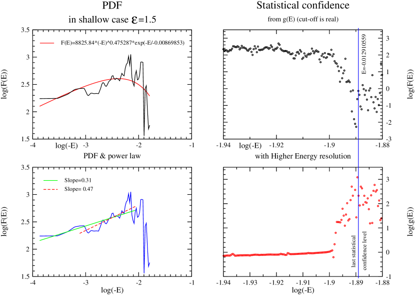
Figure 1: A shell code evaluation of the DF (Le Delliou 2001), evolved from a system with initial density $\rho\propto r^{-1.5}$. The first fit is with a cut off power law ($F\propto E^{-p}e^{-E/E_{c}}$ with $p\simeq 1/2$, $E_{c}\simeq-10^{-2}$; upper left panel), while the second fit is just a power law (lower left), confirming (HW 1999). The cut off is confirmed by higher resolution in the DF (upper right) and in density of states $g(E)$ (lower right).

In [HW 1999] weak evidence was presented to show that the $|E|^{1/2}$ law did appear near the end of the infall for the most tightly bound particles with negative energy. These would be closest to being described as occupying a rigorous steady state. A similar result was found by MacMillan [MacMillan 2006] for the most tightly bound particles even while infall continued. The case was reinforced by additional calculation of initially infinite systems by Le Delliou [Le Delliou 2001] (see Fig. 1). The figure shows another example of the Fillmore & Goldreich (1984) problem, wherein the DF (18) is a reasonable fit over most of the energy range. The cut-off is probably numerical in this case since numerically the system is ultimately finite.

However the DF (18) does not fit the complete energy distribution found in high resolution simulations of radial orbit growing isolated halos [MacMillan 2006, e.g.] in a state of self-similar virialisation [HW 1999]. In such a state, infall continues. We reserve the explanation of this behaviour to the next section where it involves the exceptional case wherein $a=1$.

Continuing for the moment with the discussion of equation (18) we observe that an upper energy cut-off is required for finiteness in the positive energy case ($a<1$ when the potential increases outwards), while the cut-off is zero in the negative energy case ($a>1$ when the potential decreases outwards). Moreover we note that one can add an arbitrary constant $E_{o}$ to $E$ in this DF, which reflects the arbitrary constant in the potential. For negative energy the DF would appear as $\widetilde{F}(E_{o}-E)^{1/2}$ for $E<E_{o}<0$. This was the type of fit used by MacMillan (2006) to fit his simulations. The DF decreases to zero at $E_{o}$ and increases to negative energy. A large positive constant $E_{o}$ and $E<E_{o}$ so that $f\propto(E_{o}-E)^{1/2}$ would express a positive energy cut-off at the value $E_{o}$ and the DF would increase towards zero energy.

The potential and density pair for these rigorously steady models take the form ($a\neq 1$)

$$\Psi=\Psi_{o}R^{(2-2a)},\leavevmode\nobreak\ \leavevmode\nobreak\ \leavevmode\nobreak\ \leavevmode\nobreak\ \leavevmode\nobreak\ \leavevmode\nobreak\ \Theta=2(3-2a)(1-a)\Psi_{o}R^{-2a}.$$ (19)

In a very recent submission Amorisco and Evans [Amorisco&Evans 2010] prove that the power-law relation between the galactic half-light radius and the central velocity dispersion in dwarf ellipticals requires a power law potential to be valid. This arises naturally here.

In the example of a dominant central point mass, inserting the index $a=3/2$ in the above pair yields a point mass surrounded by massless particles. The massless particles may be distributed in any manner, but since $\boldsymbol{d}_{N}=(0,-3)$ dimensional analysis requires that the number density $N$ should vary as $N\propto N_{o}(R)e^{-3\delta T}=N_{o}(R)R^{3}/r^{3}$. In a rigorously steady state this should be time independent so that $N_{o}(R)\propto R^{-3}$ and hence $N\propto r^{-3}$. Such a halo could exist outside any dominant mass as was discussed in [HW 1999]. Thus it might surround a central point mass or indeed be the diffuse halo around a bulge containing most of the system mass. However this is only a limiting behaviour and does not include the transition region. This region interests us particularly in the context of central black holes.

The direct density integral over the DF (18) for negative energies yields for $\rho$

$$\rho=\frac{\pi\widetilde{F}}{\sqrt{2}}\frac{|\Phi|}{r^{2}}.$$ (20)

Since this is linear in the potential, one can readily include a central mass by iteration. We may begin with a point mass potential for $\Phi$ in the density (20), and then use the Poisson equation to obtain a new potential in a form that is no longer self-similar. This yields

$$\Phi_{1}=-\frac{M_{\star}+C_{2}(1+\ln{r})}{r},$$ (21)

whence follows a new density by (20). The constant $M_{\star}$ would be the mass inside $\ln{r}=-1$ (regarded as a point mass) while $C_{2}=\left(\pi\widetilde{F}/\sqrt{2}\right)M_{\star}$. There is only a logarithmic modification to the $r^{-3}$ law at large $r$ where the iteration should apply. In effect the iteration yields a singular perturbation series at $r=0$ because of the diverging potential and hence energy. Therefore we arbitrarily cut off the series at small $r$ and ‘renormalize’ the central mass to the mass inside this cut-off radius. The next loop of the iteration gives

$$\Phi_{2}=-\frac{M_{*}(1-\frac{C_{2}^{2}}{2M_{*}^{2}})}{r}-C_{2}(1+\frac{2C_{2}}{M_{*}})\frac{(1+\ln{r})}{r}-\frac{\ln^{2}{r}}{r}\frac{C_{2}^{2}}{2M_{*}}$$

where again we have ‘renormalised’ at $\ln{r}=-1$. Putting this back into equation (20) yields $\rho_{2}$ as $r^{-3}$ flattened only by logarithmic terms at large $r$ [HW 1999] as expected. The large scale $r^{-3}$ density profile does not fit the bulge simulations inside the NFW [Navarro, Frenk & White 1996] scale length, but it does describe the halo region outside a central bulge of mass $M_{\star}$ [HW 1999].

Since the density is linear in the potential we may also solve for a self-consistent cusp having the DF (18) by letting the potential be determined by the Poisson equation. Working in transformed variables we find

$$\Psi=-AR^{p_{-}}-BR^{p_{+}},$$ (22)

where $A$, $B$ are arbitrary real constants $>0$ and

$$p_{\pm}=-\frac{1}{2}\pm\sqrt{\frac{1}{4}-\frac{\pi}{\sqrt{2}}\widetilde{F}}.$$ (23)

By letting $\widetilde{F}\rightarrow 0$ we see that $p_{-}$ is the power that should be taken near the centre if we wish to create a strong central mass concentration. It tends to $-1$ in this limit while $p_{+}$ tends to zero. Hence we set $B=0$ in this limiting domain. The potential then satisfies our basic condition (14) with a new self-similar index. This is given by $a=1-p_{-}/2$ according to equation (14), that is explicitly

$$a_{-}=\frac{5}{4}+\frac{1}{2}\sqrt{\frac{1}{4}-\frac{\pi}{\sqrt{2}}\widetilde{F}}.$$ (24)

Equation (19) now gives the inner cusp density law as

$$\Theta=|p_{-}|(1+p_{-})|\Psi_{o}|R^{(-2+p_{-})}.)$$ (25)

This can not be flatter than $R^{-2.5}$, which appears only for the ‘ maximum bulge’ for which $\widetilde{F}=1/(2\pi\sqrt{2})$. At large $r$ the term in $p_{+}$ dominates, and the behaviour tends to $r^{-2}$ for $\widetilde{F}$ small.

In the context of dark matter simulations such a steady halo of radial orbits could describe the region just beyond the NFW scale radius (which we take to form the ‘bulge’), based on the density profile alone. It is not stable in a strictly steady state according to the usual Antonov criteria [Binney & Tremaine 1987, e.g.], unless the energy is negative. Consequently we do not expect it in central regions where $a<1$ and the energy is positive (with a central zero: the potential increases outward according to Eq. 19). The radial velocity dispersion is $\overline{v_{r}^{2}}=|\Phi|/2$.

This concludes our study of the general, steady, spherically symmetric, DF for power law distributions of radial orbits. The main justification for the study is that it permits definite conclusions. The rigorously steady DF (18) is not permitted to contain a black-hole or other centralised spherical mass without perturbation. By iteration we show that it can only yield logarithmic corrections to an inverse cube law. This suggests that a black hole will engender time dependence in its surroundings.

The DF (18) also permits a self-consistent exact solution for the potential and density in the cusp (see e.g. equation 25). However it fails to produce a sufficiently flat cusp of dark matter or stars to explain observations of the Milky Way cusp of stars. At large distance it yields (at flattest) an inverse square law density.

For these reasons we turn in the next section to a time dependent case which is much more promising. It allows us to calculate the growth of a central mass due to infall of collisionless matter on radial orbits.

4 The Logarithmic Case

The case $a=1$ is obviously special and, as it turns out, rather important. We return to the equation (13) and observe that we also have an integral in the steady state if $\psi=\psi_{o}\ln{R}$. For in that case the equation integrates to $\mathcal{E}+\psi_{o}\alpha T=\kappa$, where $\kappa$ is constant on the characteristic. Equation (16) then requires that in general $F=F(\kappa)$, so $F$ is also constant on the characteristic. With $a=1$ we note from equation (3) that $\Psi\equiv\Phi$, $Y\equiv v_{r}$ and so $\mathcal{E}\equiv E$. However $\kappa=v_{r}^{2}/2+\psi_{o}\ln{R}+\alpha T=v_{r}^{2}/2+\psi_{o}\ln{r}\equiv E$ and moreover $\pi f\equiv F$. Hence our conclusion is for the moment only that

$$\pi f=F(E),$$ (26)

in this case.

By taking the potential to be logarithmic, $\Psi=\Psi_{o}\ln{R}$, we require by equation (6) that $\Theta=\Psi_{o}/R^{2}$ and hence, by the appropriate members of the set (3), that $\rho=\Psi_{o}/r^{2}$. But for consistency we must also have

$$\rho=\frac{\Psi_{o}}{r^{2}}=\frac{1}{r^{2}}\int\leavevmode\nobreak\ F(E)\leavevmode\nobreak\ \mathrm{d}v_{r}.$$ (27)

We must therefore find a DF $F(E)$ which satisfies this equation. In effect, the integral over the particle velocities must be a constant independent of the logarithmic potential.

To find such a DF we convert the integral to an integral over energy in the normal fashion and write our consistency condition as

$$I\equiv\sqrt{2}\int\leavevmode\nobreak\ \frac{F(E)}{\sqrt{(E-\Phi)}}\leavevmode\nobreak\ dE=\Psi_{o}.$$ (28)

We might expect a power law form for $F(E)$ on general grounds, and given this a brief experimentation shows that the most general form for $F(E)$ in this case may be written as (we suppose negative energy to ensure convergence and $E<E_{o}<0$ where $E_{o}$ is an arbitrary constant energy)

$$F(E)=\frac{K}{\sqrt{(E_{o}-E)}}$$ (29)

This may also be inferred as the unique solution with a finite energy range by recognizing that equation (28) is really a simple form of Abel’s integral equation (see e.g. [Binney & Tremaine 1987] in the first or finite form, p651) whose solution is equation (29) with

$$K=\frac{\Psi_{o}}{\sqrt{2}\pi}.$$ (30)

This may be checked by direct evaluation of the integral to find that $\rho=\Psi_{o}/r^{2}$ as required.

This result holds only where $E<0$ and hence where $r<r_{o}$, where $r_{o}$ is an arbitrary scale. However since we have not actually set a fixed scale in the problem (which would entail setting $\delta=0$), we have implicitly implied that $r/r_{o}=R/R_{o}$. Thus we have assumed that $r_{o}=R_{o}e^{\alpha T}=\alpha R_{o}t$. We may take $R_{o}$ constant (dimensionless) so that there is a residual time dependence because the outer boundary expands according to $r_{o}=R_{o}e^{\alpha T}$. This implies that the mass inside $R_{o}$ and indeed inside any fixed $R$ is growing as $M=4\pi\Psi_{o}R\alpha t$.

We have thus succeeded according to the above in deriving the Fridmann and Polyachenko DF [Fridmann & Polyachenko 1984] as the unique result of time-dependent radial accretion of a growing inverse-square density ‘bulge’. This is one of our major conclusions.

A numerical measure of the DF in radial self-similar continuing infall was made by MacMillan [MacMillan 2006]. Instead of the steady DF, the DF of Fridman and Polyachenko [Fridmann & Polyachenko 1984] is found to predict accurately all of the measured quantities as in the accompanying figures. These include an inverse square density law and a power law pseudo-phase-space density of $\approx-1.5$, but there are logarithmic corrections to the power law as can be calculated from the FP distribution function. The pseudo-phase-space density power is flatter [MWH 2006, i.e. MacMillan, Widrow & Henriksen 2006] than is generally found in full cosmological simulations. These results are illustrated in figures (2) and (3).

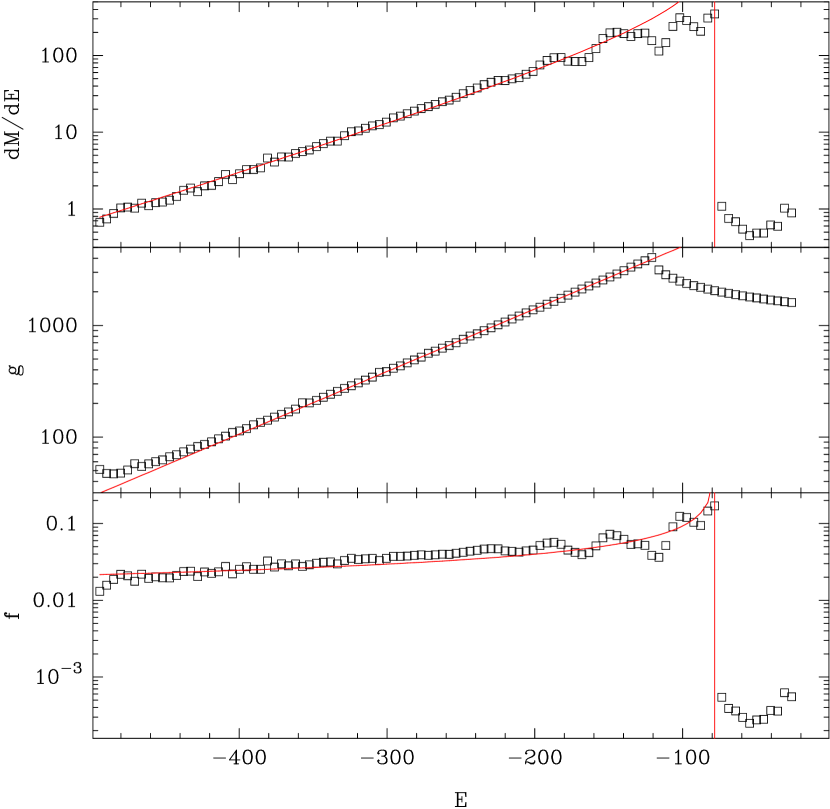
Figure 2: We show the Fridman and Polyachenko fit to the mass distribution $dM/dE=f(E).g(E)$, density of states $g(E)$, and the phase space distribution function $f(E)$. The figure is based on the radial simulations of an isolated dark matter halo by (MacMillan 2006). The system is maintained in self-similar virialisation by steady accretion. The fits use equation (31) with $K=-E_{o}/(4\sqrt{2}\pi^{3})$ and $E_{o}\approx-80$ in machine units.

This DF [Fridmann & Polyachenko 1984] used to make the fits in figures (2) and (3) is

$$f=\frac{K}{(-E+E_{o})^{1/2}}\delta(j^{2}),$$ (31)

for $E<E_{o}\leq 0$, and $r\leq r_{f}$ (where $\Phi(r_{f})=E_{o}$) and zero otherwise. This is just as we inferred above. The density profile is $r^{-2}$ and the potential is logarithmic. The logarithmic variation of the velocity dispersion together with the inverse square density profile accounts for the pseudo density approximate power law found in the simulations [MacMillan 2006].

The persistence of this DF is undoubtedly due to the strict proscription of non-radial forces in the simulations. It is not linearly stable by the Antonov criteria for $E<0$. When this proscription is relaxed [MacMillan 2006] shows that the equilibrium Fridman and Polyachenko DF is subject to the radial orbit instability. It may require continual non-equilibrium excitation as provided by steady infall to be realized.

The unique feature of the distribution function (31) is that the density is independent of the potential. Hence one can simply add a point mass potential to the logarithmic bulge value and the density will remain $\Psi_{o}r^{-2}$. In the case of a true absorbing central black hole one should only permit negative radial velocities in the system. This means that $K$ in equation (30) should be multiplied by a factor $2$. The velocity dispersion however goes as $\overline{v_{r}^{2}}=|\Phi-E_{o}|$ and we may take $\Phi=-M_{\star}/r+\sqrt{2}\pi K\ln{r}+E_{o}$. MacMillan (2006) finds a good fit to this radial dispersion in his simulations, but without a central mass.

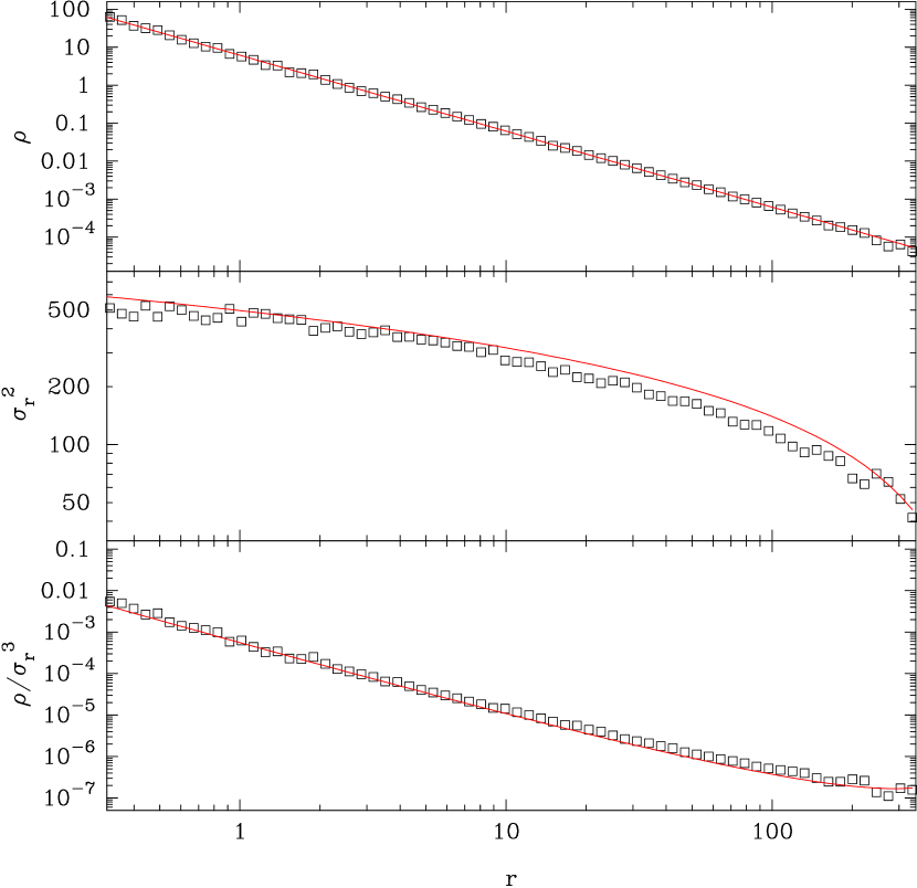
Figure 3: We show the the Fridman and Polyachenko fit to the mass density, the velocity dispersion and the ‘pseudo-phase-space density’ for the same simulations by MacMillan.

The actual growth of the black hole mass will be simply that of the general self-similar mass growth as discussed above. That is

$$M_{*}(t)=M_{*}(0)e^{\alpha T}=M_{*}(0)\alpha t.$$ (32)

Its radius will be growing according to the same law.

One can not however take seriously the growth of a black hole due to radially infalling material from cosmological distances, since the material there can not know the actual location of the black hole and the radial infall is subject to the radial orbit instability. However, as we will speculate in the discussion section, such growth may apply to a hierarchy of ‘central’ masses extending to ever smaller scales. That is $M_{*}$ might be successively the bulge of a galaxy, the core, the nucleus, and so on to the black hole. In each case there must be a way of scattering orbits into the essentially radial loss cone. Such scattering may be due in part to the formation of a bar by the radial orbit instability itself, or to clump-clump interaction.

It is worth contrasting the above infall time-dependent DF with the rigorously steady system of radial orbits in spherical symmetry. This case was inadvertently omitted in the discussion by [HW95] and so we pause to present it in our general style as another example of the method, similar to that above but in a strictly steady state.

The main difference with the time dependent case is that that the scaling motion must be taken in space rather than in time. This means that we use the variable $R$, where $e^{\delta R}\equiv\delta r$ so that $dR/dr=e^{-\delta R}$. In addition we write

$$f=F\delta(v_{\theta})\delta(v_{\phi}),$$ (33)

where $F$ satisfies [integrate the general steady CBE in spherical symmetry [Binney & Tremaine 1987] over $v_{\theta}$ and $v_{\phi}$]

$$v_{r}\frac{\partial F}{\partial r}-\frac{\partial\Phi}{\partial r}\frac{\partial F}{\partial v_{r}}+\frac{2Fv_{r}}{r}=0.$$ (34)

In addition we have the Poisson equation as

$$\frac{1}{r^{2}}\left[\frac{\mathrm{d}}{\mathrm{d}r}\left(r^{2}\frac{\mathrm{d}\Phi}{\mathrm{d}r}\right)\right]=\rho=\int\leavevmode\nobreak\ F\leavevmode\nobreak\ \mathrm{d}v_{r}.$$ (35)

The dimension vectors in our usual scaling space are $\boldsymbol{d}_{F}=(1,-4,1)$, $\boldsymbol{d}_{v}=(-1,1,0)$,$\boldsymbol{d}_{\rho}=(0,-3,1)$ and $\boldsymbol{d}_{\Phi}=(-2,2,0)$. Recalling that $\mu=3\delta-2\alpha$ the vector for $F$ becomes $(-1,-1)$, the vector for $\rho$ becomes $(-2,0)$ while the others remain unchanged in the reduced $(\alpha,\delta)$ space. However we will only consider the case $a=1$ or $\alpha=\delta$ since the other cases were discussed in [HW95] and reduce to the DF (18). When $\alpha=\delta$ the dimension vectors reduce in delta dimension space to $(-2)$, $(-2)$, $(0)$ and $(0)$ respectively. Hence the equivalent of equation (3) is

$$\delta r =e^{\delta R}, Y =v_{r},$$

$$e^{-2\delta R}P\left(R,Y\right) =F\left(r,v_{r}\right),$$ (36)

$$\Psi\left(R\right) =\Phi(r,t),$$

$$e^{-2\delta R}\Theta\left(R\right) =\rho(r).$$

If self-similarity is enforced normally, then in this case $\partial_{R}=0$ when it acts on the scaled variables. However this can not apply to $\Psi(R)=\Phi$ since then equation (34) becomes trivial. The answer lies in the realization that in this case the potential is logarithmic in $r$, rather than being a power law. The condition $\alpha=\delta$ requires that there be a constant $\Psi_{o}$ with dimensions of the potential per unit mass, just as in the time dependent case. These conditions are satisfied here by setting

$$\Psi(R)=\Psi_{o}(\delta R)\equiv\Psi_{o}\ln{\delta r}=\Phi(r).$$

Since only $\partial_{R}\Psi$ appears in the problem, the self-similar requirement of independence of $R$ is maintained for $F$.

A direct substitution of the transformation (36) plus the form of the potential into equation (34) reduces it to

$$Y\partial_{R}P-\frac{\mathrm{d}\Phi}{\mathrm{d}R}\partial_{Y}P=0$$

and hence after solving by characteristics

$$P=P(E)$$

Consequently we find finally from $F=Pe^{-2\delta R}\equiv P/(\delta r)^{2}$ the steady density in the form

$$\rho=\frac{1}{\delta^{2}r^{2}}\int\leavevmode\nobreak\ P(E)\leavevmode\nobreak\ \mathrm{d}v_{r},$$ (37)

where

$$E\equiv\frac{v_{r}^{2}}{2}+\Phi(R).$$

From the Poisson equation (35) we obtain

$$\rho=\frac{\Psi_{o}}{r^{2}},$$

and this must agree with the integral over $F$. Letting both inward and outward going particles be present one finds that

$$\rho=\frac{\sqrt{2}}{\delta^{2}r^{2}}\int\leavevmode\nobreak\ \frac{P(E)}{\sqrt{(E-\Phi)}}\leavevmode\nobreak\ \mathrm{d}E.$$

The problem is now reduced to the same situation that we had in the time dependent case found earlier (27 and following). In order to have a consistent (with the Poisson equation) inverse square density law, only the steady Fridmann and Polyachenko DF may be invoked, and that only for negative energies wherein $\Phi<E<E_{o}$. Thus we derive the finite and steady Fridman and Polyachenko result as quoted for example in [Binney & Tremaine 1987].

5 Discussion and Conclusions

In this paper we have presented unique distribution functions based on the self-similar evolution of a gravitating system of radial orbits. The rigorously steady state corresponds to an infinite system while the time dependent system is finite and growing. Both of these systems have been confirmed by numerical simulations, with the confirmation of the growing mode being most dramatic.

Both systems have been derived coherently from the basic equations by using a convenient formulation of self-similarity. We have considered how these distributions are affected by the presence of a central spherical mass, which may not necessarily be point-like. The steady system is perturbed outside the central mass to an inverse cube law with logarithmic corrections as we discuss further below. The growing time-dependent case forms a perfect inverse-square density cusp that can contain a central mass and is growing proportionally to the time since formation. The material with which we are concerned is collisionless and so may refer to dark matter in an early stage of formation or to stars at a later stage. The restriction to radial orbits in this paper is removed in subsequent papers, although both in theory and in the numerical simulations a bias to radial orbits remains on the larger scales.

For this latter reason we think that the results of this paper may be relevant in reality for two reasons. In the first instance the distribution functions may develop outside a rapidly formed large central bulge wherein angular momentum has been important. This may correspond to the NFW core radius, and our detailed results are compatible with the density profile of the simulations outside this radius. The second plausible scenario is that, on much smaller scales surrounding an actual black hole, various instabilities may allow radial infall of stars and dark matter onto the centre. This fits the time-dependent infall model and allows the black hole to grow proportionally to the time from the onset of the radial infall. We detail these results in what follows.

In section (3) on the steady state we deduced the steady, spherically symmetric DF with radial orbits that yields infinite systems with power law profiles. This was found previously but we rederive it here as a limit of the time-dependent equations. We have perturbed this DF by embedding a central mass. The DF is universal for these systems ($f=K|E_{o}-E|^{1/2}$) but the potential-density pair depends on the self-similar index $a$ which in turn depends on dominant constants or boundary conditions. If it is a memory of a cosmological fluctuation profile, then $a=3\epsilon/(2(\epsilon+1))$.

This steady DF can not contain a central mass without being perturbed, except for the Keplerian limit wherein $a=3/2$ and there is a mass-less cusp with an inverse cube density profile. Iterating the equations to find the perturbation produced by an embedded central mass predicts a transition region in the halo of the mass that is an $r^{-3}$ profile modified only by logarithmic corrections. It does not correspond to the power law density of stars found close to the black hole in the galactic centre[Gillessen et al., 2009], but may apply outside a bulge mass confined to the NFW scale radius.

Since the density is linear in the potential we were also able to find a solution that broke the self-similarity by seeking non-power-law solutions of Poisson’s equation (pure power laws only exist in the limits) with the density (20). The density profile of the cusp can not be flatter than $r^{-2.5}$ near a central point mass, but it may be as flat as $r^{-2}$ at large scales in the low density limit. Such behaviour is too steep to explain the cusp observed around the Sagittarius A* black hole. All possible descriptions of a steady system of radial orbits are clearly excluded by this observation. These descriptions are not excluded outside a central bulge however.

In the section concerning the logarithmic potential exception we showed that it corresponded to continuing time-dependent infall. We found both theoretically and numerically that the Fridmann and Polyachenko DF is the distribution established by continuing radial infall. Remarkably, it allows a growing central point mass (or indeed a bulge mass on a larger scale) to be embedded in the infall self-consistently. In both the steady and the time-dependent cases the density profile is $r^{-2}$. The time-dependent logarithmic case allows a consistent calculation of the central mass growth rate according to $M_{*}\propto t$. Such a growth rate from a surrounding envelope was found in [MacMillan & Henriksen 2003]. This simulation used a true N-body code that treated particle-particle scattering, which scattering led eventually to radial infall of some of the particles.

The growth rate of a central mass (i.e. a collisionless concentration, not a true black hole) from a reservoir of radial orbits is zero if there is a rigorous steady state. The growth rate is not zero if the central mass is a black hole, since then the outward bound radial orbits are suppressed. In that case however the steady state is only an approximation except in an infinite system. For a finite system the true timescale would be the free-fall time of the bulk of the accreting mass.

One is inclined not to take these growth estimates seriously, since they simply assume an endless supply of radial particles, and hence an arbitrarily filled loss cone. In fact the radial alignment required to hit a growing black hole from a few hundred parsecs is at least one part in $10^{8}$ to $10^{10}$ depending on the mass of the black hole! This suggests that instead [MacMillan & Henriksen 2003, see e.g.] the actual growth involving radial orbits may be by way of a multi-stage process. In the first stage, radial orbits accrete from the galactic halo to form a bound spherical bulge of intermediate size, due to finite angular momentum about the centre [MacMillan & Henriksen 2003]. They are trapped there either by the usual mechanism of self-similar infall as the potential increases in time with increasing internal mass, or by dissipative interactions. If there is substructure in the collisionless matter (e.g. stars and dark matter clumps), then these are able to produce dissipational collisions. Ultimately these collisions and tidal interactions can lead to a more gradual growth of a more central mass [MacMillan & Henriksen 2003, e.g., in the Carnegie meeting].

Recently a high resolution study [Stadel et al 2009] of sub-structure in an isolated halo revealed that this sub-structure disappears in the inner few parsecs. this coincides with the region where the halo is becoming spherical and where the density power-law is flattening to less that $1$. The interactions leading to the sub-structure disappearance may well lead to relaxation.

In addition the radial orbit instability can lead to the development of a bar [MWH 2006]. This bar can then transport angular momentum away from the bulge by the ejection of particles. Such ‘interrupted accretion’ may repeat several times on the way to the actual central object. The rapid accretion of a bulge is in fact the way in which dark matter halos are thought to grow [Zhao et al., 2003, Lu et al. 2006] initially. This is then followed by a slower growth phase. The DF (31) can be used to describe the environment of the central mass on each scale of the interrupted cascade.

In this connection we refer to the work of Mutka [Mutka 2009] on gravitationally lensed galaxies with double images. He concludes that there are two classes of density cusps with the larger sample (about 80%) showing a logarithmic density slope of $\approx-1.95$ well inside the NFW scale radius. The other 20% show this slope as $\approx-1.45$. These may be unresolved triple image lens and ,if so, the measured value should be rejected.

Mutka’s result is a measure of the total mass distribution rather than just the dark matter. Perhaps we are seeing enhanced relaxation in the mixture of stars and dark matter, that leads towards an isothermal cusp, rather than the shallower cusps of the dark matter simulations. It is significant that this inverse square slope is also frequently found by direct dynamical modeling of galaxies [van der Marel 2009].

However an inverse square slope is not restricted to a system of purely radial orbits as the isotropic isothermal distribution shows. In a subsequent paper we survey anisotropic distribution functions in spherical spatial symmetry that also have a self-similar memory. Some of these also provide an inverse square density profile.

The significance of the hierarchy of co-evolving structures is that there will always be a mass correlation between them. Thus if the mass concentration derives its ultimate mass $M_{\bullet}$ from a halo of radius $r_{h}$, while $r_{s}$ encloses the mass that forms the ultimate bulge mass $M_{s}$ then

$$\frac{M_{\bullet}}{M_{s}}=\frac{r_{h}}{r_{s}}.$$ (38)

This assumes the pure inverse square density law, which might in fact have a logarithmic correction. In the subsequent paper, we shall find a slightly more general correlation that involves the self-similar memory. Taken at face value this simple relation gives $r_{h}/r_{s}\approx 100$.

This paper comprises a systematic derivation of the distribution functions that arise through self-similar evolution of gravitating systems of radial orbits. In addition we have studied the effects of a central mass on these distributions. We do not find density profile as flat as those proposed in [Merritt & Szell 2006] and [Nakano & Makino 1999] as a result of density scouring by merging black holes. Thus our calculations probably do not describe the cusp around Sagittarius A*, although this does not exclude other applications. Subsequent papers in this series address this problem by allowing anisotropy in velocity space.

6 Acknowledgements

RNH acknowledges the support of an operating grant from the Canadian Natural Sciences and Research Council. The work of MLeD is supported by CSIC (Spain) under the contract JAEDoc072, with partial support from CICYT project FPA2006-05807, at the IFT, Universidad Autonoma de Madrid, Spain

References

- [Amorisco&Evans 2010] Amorisco N. C., Evans N. W., 2010, preprint (arXiv:1009.1813A)
- [Bahcall & Wolf 1976] Bahcall J., Wolf R. A., 1976. ApJ, 209, 214
- [1985] Bertschinger E., 1985, ApJS, 58, 39
- [Bicknell & Henriksen 1979] Bicknell G. V., Henriksen R. N., 1979, ApJ, 232,670
- [Binney & Tremaine 1987] Binney J., Tremaine S., 1987, Galactic Dynamics. Princeton Univ. Press, Princeton, NJ
- [Carter & Henriksen,1991] Carter B., Henriksen R. N., 1991, J. Math. Phys., 32, 2580
- [Diemand et al., 2006] Diemand J., Kuhlen M., Madau P., 2006, ApJ, 667,859
- [Ferrase & Merritt 2000] Ferrarese L., Merritt D., 2000, ApJ, 539, L9
- [Fillmore & Goldreich, 1984] Fillmore J. A., Goldreich P., 1984, ApJ, 281, 1
- [Fridmann & Polyachenko 1984] Fridman A. M., Polyachenko V. L., 1984, Physics of Gravitating Systems, Springer-Verlag, New York (FPDF)
- [Fujiwara 1983] Fujiwara T., 1983, PASJ, 35, 547
- [Gebhardt et al., 2000] Gebhardt K. et al., 2000, ApJ, 539, L13
- [Gillessen et al., 2009] Gillessen S., Eisenhauer F., Trippe S., Alexander T., Genzel R., Martins F., Ott T., 2009, ApJ, 692, 1075
- [H2004] Henriksen R. N., 2004, MNRAS, 355, 1217
- [Henriksen 2006a] Henriksen R. N., 2006a, MNRAS, 366, 697
- [H2006] Henriksen R. N., 2006b, ApJ, 653,894 (H2006)
- [H2009] Henriksen R. N., 2009, ApJ, 690, 102
- [HLeD 2002] Henriksen R. N., Le Delliou M., 2002, MNRAS, 331, 423
- [HW95] Henriksen R. N., Widrow L. M., 1995, MNRAS, 276, 679 (HW95)
- [HW 1999] Henriksen R. N., Widrow L. M., 1999, MNRAS, 302, 321(HW1999)
- [Graham 2004] Graham, A., 2004, ApJ, 613, L33
- [Kormendy & Bender 2009] Kormendy J., Bender R., 2009, ApJ, 691,L142
- [Kormendy & Richstone 1995] Kormendy J., Richstone D., 1995, ARA&A, 33, 581
- [Kurk et al., 2007] Kurk J. D. et al., 2007, ApJ, 669, 32
- [Le Delliou 2001] Le Delliou, M., 2001, PhD Thesis, Queen’s University, Kingston, Canada
- [I] Le Delliou M., Henriksen R. N., MacMillan J. D., 2010a, preprint (arXiv:0911.2232) (paper I)
- [II] Le Delliou M., Henriksen R. N., MacMillan J. D., 2010b, A&A, 522, A28 (paper II)
- [III] Le Delliou M., Henriksen R. N., MacMillan J. D., 2011, A&A, 526, A13 (paper III)
- [Lu et al. 2006] Lu Y., Mo H. J., Katz N., Weinberg M. D., 2006, MNRAS, 368, 1931
- [Lynden-Bell 1967] Lynden-Bell D., 1967, MNRAS, 36, 101
- [MacMillan 2006] MacMillan J., 2006, PhD Thesis, Queen’s University at Kingston, Canada
- [MacMillan & Henriksen 2002] MacMillan J. D., Henriksen R. N., 2002, ApJ, 569, 83
- [MacMillan & Henriksen 2003] MacMillan J. D., Henriksen R. N., 2003, in Collin S., Combes F. and Shlosman I., eds., Meudon, France, ASPC Proceedings, 290, 213
- [MWH 2006] MacMillan J. D., Widrow L. M., Henriksen R. N., 2006, ApJ, 653, 43 (MWH 2006)
- [Magorrian et al. 1998] Magorrian J. et al., 1998, AJ, 115, 2285
- [Maiolino et al. 2007] Maiolino R. et al., 2007, A&A, 472, L33
- [Merritt & Szell 2006] Merritt D., Szell A., 2006, ApJ, 648, 890
- [Mutka 2009] Mutka P., 2010, in Alimi J.-M., ed., Paris, France, AIP Conference Proceedings, 1241, 244.
- [Nakano & Makino 1999] Nakano T., Makino M., 1999, ApJ, 525, L77
- [Navarro, Frenk & White 1996] Navarro J. F., Frenk C. S., White S. D. M., 1996, ApJ, 462, 5
- [Peebles 1972] Peebles P. J. E., 1972, Gen. Relativ. Gravit., 3, 63
- [Peirani & de Freitas Pacheco 2008] Peirani S., de Freitas Pacheco J. A., 2008, Phys. Rev. D, 77, 064023
- [Quinlan et al 1995] Quinlan G. D., Hernquist L., Sigurdsson S., 1995, ApJ, 440, 554
- [Stadel et al 2009] Stadel J., Potter D., Moore B., Diemand J., Madau P., Zemp M., Kuhlen M., Quilis V., 2009, MNRAS, 398, L21
- [ Van den Bosch et al. 2008] Van den Bosch R. C. E., van de Ven G., Verolme E. K., Cappellari M., de Zeeuw P. T., 2008, MNRAS, 385, 647
- [van der Marel 2009] van der Marel, R., 2009, in S. Courteau ed., Unveiling the Mass. Queen’s University, Kingston, Ontario, Canada
- [Walter et al., 2009] Walter F., Riechers D., Cox P., Neri R., Carilli C., Bertoldi F., Weiss A., Maiolino R., 2009, Nature, 457, 699
- [Young 1980] Young P., 1980, ApJ, 242, 1232
- [Zhao et al., 2003] Zhao D. H., Mo H. J., Jing Y. P., Börner G., 2003, MNRAS, 339. 12