A Robust Control Framework for Malware Filtering

Abstract

We study and develop a robust control framework for malware filtering and network security. We investigate the malware filtering problem by capturing the tradeoff between increased security on one hand and continued usability of the network on the other. We analyze the problem using a linear control system model with a quadratic cost structure and develop algorithms based on H^∞-optimal control theory. A dynamic feedback filter is derived and shown via numerical analysis to be an improvement over various heuristic approaches to malware filtering. The results are verified and demonstrated with packet level simulations on the Ns-2 network simulator.

I Introduction

Attacks on computer networks, such as worm or denial of services attacks, are difficult to prevent in part due to the challenge of detecting and stopping them while still allowing legitimate network usage. Recent experience with Internet worm attacks makes this point more clear: within 10 minutes the Slammer worm had infected 90% of vulnerable computers in 2003 and the Code Red virus infected hundreds of thousands of hosts in 2001 [1, 2]. The base-rate fallacy captures the essence of this problem. Even if we have low false-negative and false-positive rates in our detection of malware, there is so much more legitimate network usage than illegitimate usage that we end up with many false alarms [3]. The incredible variety in legitimate network traffic makes accurately differentiating it from malicious traffic even more challenging. A more detailed analysis of the detection of a particular type of worm epidemic in  [4] shows the challenge of detecting some worm attacks even under idealized conditions. In this specific case the base-rate fallacy again comes into play, as “a substantial volume of ‘background radiation’” is to blame for making the detection of random constant scanning worms difficult. Intrusion detection systems must be constructed with this dilemma in mind, and thus need to be conservative in their operation.

According to Federal Bureau of Investigation (FBI) statistics, 70% of security problems originate within an organization, and 20% of respondents to an FBI survey indicated that intruders had broken into or attempted to break into their corporate networks in the last 12 months [5]. Therefore, dynamic firewalls such as the Cisco Internetwork Operating System (IOS) firewall are an important form of internal network security [5]. Our aim is to develop algorithms and policies for such (re)configurable firewalls in order to filter malware traffic such as worms, viruses, spam, and Trojan horses.

We use $H^{\infty}$-optimal control theory to determine how to dynamically change filtering rules or parameters in order to ensure a certain performance level. We note that in $H^{\infty}$-optimal control, by viewing the disturbance as an intelligent maximizing opponent in a dynamic zero-sum game, who plays with knowledge of the minimizer’s control action, one evaluates the system under the worst possible conditions. This approach applies naturally to the problem of malware response because the traffic deviation resulting from a malware attack is not merely random noise, but represents the efforts of an intelligent attacker. Therefore, we determine the control action that will minimize costs under these worst circumstances [6]. The resulting conservative controller works well even in light of the base-rate fallacy problem. To the best of our knowledge, this work represents the first application of robust control theory to the problem of malware filtering.

I-A Related work

There are several methods of dynamic packet filtering [7]. Perhaps the most common one is to dynamically change which ports are open or closed. Stateful inspection of deeper layers of packets allows for even more detailed filtering by creating and maintaining information about the state of a current connection [5]. Another possibility is to dynamically alter the set of Internet Protocol (IP) addresses from which traffic will be accepted [8]. An accurate attack packet discarding scheme based on statistical processing has been proposed in [9], where each packet is associated with a score that reflects its legitimacy. Once the score of a packet is computed, this scheme performs score-based selective packet discarding where the dropping threshold is dynamically adjusted based on the score distribution of recent incoming packets and the current level of system overload.

Implicit to the network traffic filtering problem considered in this article is the partitioning of a computer network into various sub-networks for administrative and security purposes. This approach is common, and a separate firewall is often assigned to each sub-network. Zou et al. [10] have proposed a “Firewall Network System” based on this very concept. Cisco recommends their IOS firewalls for defending particular sub-networks or LANs in a corporate network [5]. In  [11], quarantining these sub-networks is considered as a strategy to slow the spread of worm epidemics. We note that although the algorithms developed in this paper can be helpful for configuring dynamic firewalls such as the ones described above, our main objective is to develop mathematical foundations and algorithms for future security systems which will be even more configurable and flexible. Finally, while we consider the case of filtering packets, these techniques could also be applied to filtering connections.

The remainder of this article is structured as follows: Section II discusses the problem of filtering network traffic with dynamic firewalls separating sub-networks. We next derive the $H^{\infty}$-optimal controller and state estimator in Section III. Section IV reviews Matlab and Ns-2 simulations of the H^∞-optimal controller and demonstrates its performance in comparison with other controllers. Concluding remarks and directions for future research are presented in Section V.

II Network Traffic Filtering Model

In this section we present a linear system model for malware traffic and study the problem of filtering network traffic to prevent malware propagation. Consider a computer network under the control of a single administrative unit, such as a corporate network. Assume the network is divided into sub-networks for administrative and security purposes [5]. While we will describe the model within this context, the corresponding control framework can be applied to other contexts by redefining the entities in question.

Let $x(t)$ represent the number of malware packets that traverse a link on their way to the destination sub-network at time $t$ originating from infected sources outside the sub-network. We model this malware flow to the sub-network using a linear differential equation with control and disturbance terms:

$$\dot{x}(t)=a\,x(t)+b\,u(t)+w_{a}(t),$$ (1)

where $u(t)$ represents the number of packets that are filtered at a particular time $(t)$. Usually, only some proportion of the packets filtered are actually malware related. Thus, the parameter $b$ corresponds to that proportion multiplied by $-1$. In other words, $(1-b)$ is the proportion of filtered packets that are not malware related. On the other hand, $w_{a}(t)$ represents the number of malware packets added to the link at time $t$ intentionally by malicious sources or unintentionally by hidden software running on hosts, both located outside the sub-network considered. Thus $u(t)$ and $w_{a}(t)$ represent, for this specific sub-network, the packet filtering rate and malware infiltration rate, respectively. The $a$ value represents the instantaneous proportion of malware packets on the link that are actually delivered to the sub-network and is thus a negative number.

Expanding the dimensions of the model in (1) leads to a set of linear differential equations:

$$\dot{\mathbf{x}}(t)=A\mathbf{x}(t)+B\mathbf{u}(t)+D\mathbf{w}_{a}(t),$$ (2)

where $\mathbf{w}_{a}$ is defined as the vector of malware packets. In this case both $A$ and $B$ are obtained simply by multiplying the identity matrix by $a$ and $b$, respectively. The $D$ matrix imposes a propagation model on the attack and quantifies how malware is routed and distributed on this network. For the purposes of this paper, it has zeros for its diagonal terms (intra-sub-network malware traffic does not leave the sub-network), and each column must sum to 1 to ensure conservation of packets. In this version of the problem, the malware being sent to sub-network $i$ is a function of $w_{j}$ for $j\neq i$, the malicious traffic generated by other sub-networks. This assumption on the propagation of malware inherent to the form given to $D$ allows for a centralized filtering solution that considers network-wide conditions. A decentralized version to this problem is also possible, however. Overall, this model simplifies actual network dynamics by assuming a linear system and using a fluid approximation of traffic flow.

Let us denote by $\mathbf{y}(t)$ our measurement of the number of inbound malicious packets prior to filtering. Note that the separation between detection ($\mathbf{y}(t)$) and response ($\mathbf{u}(t)$) is only at the conceptual level. In the implementation both may occur on the same device. Inaccuracies in $\mathbf{y}(t)$ are inevitable due to the challenging problem of distinguishing malicious packets from legitimate ones [3]. To capture this uncertainty formally, we define $\mathbf{y}(t)$ as

$$\mathbf{y}(t):=C\mathbf{x}(t)+E\mathbf{w}_{n}(t),$$ (3)

where $\mathbf{w}_{n}(t)$ is measurement noise of any form. Later, we derive and apply the worst-case measurement noise $\mathbf{w}_{n}(t)$. Additionally, we define $N:=EE^{T}$ and assume that it is positive definite, meaning that the measurement noise impacts each dimension of the measured output. The $C$ matrix models the assumption that $\mathbf{y}(t)$ is higher than and proportional to $\mathbf{x}(t)$. When implemented, entries of this constant matrix could be measured from an analysis of packet filtering and the calculations required for determining the optimal controller could be rerun periodically.

Note that we do not make any assumption on how $\mathbf{y}(t)$ is obtained. It could be the result of some statistical analysis comparing the expected traffic to the measured traffic or be based on a set of rules where packets with certain characteristics are assumed to be malicious.

Similarly, $\mathbf{w}_{a}(t)$ represents a worm attack, expressed in terms of number of the malware packets sent from a sub-network to other sub-networks at each time instant. More precisely, it is the generated malware traffic flow rate in terms of packets per time step. For example, if a worm is very rapidly contacting new hosts and sending them packets, then $\mathbf{w}_{a}(t)$ would be large. However, we do not assume any form on the attack. To simplify notation, we assume that the measurement noise and attack disturbance are both part of the vector $\mathbf{w}:=\left[\mathbf{w}_{a}^{T}~{}\mathbf{w}_{n}^{T}\right]^{T}$.

The model at hand contains several simplifications and assumptions. As was mentioned earlier, the components of the $B$ matrix are set to be constants, although in reality the value of these components should change as $\mathbf{x}$ decreases, as there are less malicious packets to be filtered, and we are filtering packets we are less sure about. This quantity also depends on the amount of legitimate network traffic on the link: if there is a relatively large amount of legitimate network traffic then we will incur more false-positives and thus end up filtering more legitimate traffic. The $B$ matrix is related to the false-negative and false-positive ratios, but it is mostly determined by the ratio of legitimate to illegitimate traffic as described in  [3]. The exponential decay in the number of malware packets on the link (in the absence of control and disturbance) does not exactly capture network dynamics, but with a high enough rate of exponential decay, this assumption is quite realistic when capacity constraints are not significant. The assumption of a constant value for the $C$ matrix is also an approximation, as in reality the number of malware packets prior to filtering will probably not be linearly dependent upon the number after filtering. To summarize, this model simplifies actual network performance by assuming linear dynamics.

Moreover, this model simplifies system dynamics by using a fluid approximation of traffic flow. More specifically, this model only approximately captures the fact that, in an actual implementation, the number of malware packets measured prior to filtering differs from the one that arrives at the sub-network in the number of the filtered. Similarly, in order to simplify the following calculations, we are approximating a clearly discrete and event-driven system (a computer network) with a continuous time system. This assumption should hold when we consider the rapidity and frequency of packet arrivals and transmissions along with the fine-grained time increments of a computer network.

III Derivation of Optimal Controller and State Estimator

Our objective now is to design an algorithm or controller for traffic filtering given this imperfect measure of inbound malicious packets. As part of the $H^{\infty}$-optimal control analysis and design we introduce first the controlled output

$$\mathbf{z}(t):=H\mathbf{x}(t)+G\mathbf{u}(t),$$ (4)

where we assume that $G^{T}G$ is positive definite, and that no cost is placed on the product of control actions and states: $H^{T}G=0$. $H$ represents a cost on malicious packets arriving at a sub-network. A few other constraints that must be met for this $H^{\infty}$-optimal control theory to apply are that $(A,\,B)$ and $(A,\,D)$ be stabilizable, and $(A,\,H)$ and $(A,\,C)$ be detectable, and these conditions readily hold in our case.

If $\mathbf{x}$ becomes negative, we are filtering legitimate packets from the link. In other words, an equal penalty is assumed for underfiltering and allowing worm-related traffic on a link and also for overfiltering and preventing legitimate network traffic from traversing the link. By weighting these two quantities equally, we are in effect encouraging survivability: overfiltering to prevent the spread of the worm but at the same time crippling the network is penalized as much as allowing the worm-related traffic to run rampant.

The cost on filtering legitimate traffic is actually more complicated than indicated above. Recall that $b$ specifies the proportion of filtered traffic that is malware-related. Thus, $(1-b)$ is the proportion of filtered traffic that is legitimate (assuming $\mathbf{x}$ is positive). If we assign a cost of $f_{l}$ to filtering legitimate packets when malware packets are on the link and a cost of $f_{a}$ to the filtering action itself, the components $g$ of $G$ can be specified as $g=f_{l}(1-b)+f_{a}$.

The cost of this system for the purpose of $H^{\infty}$ analysis is defined by

$$L(\mathbf{x},\mathbf{u},\mathbf{w})=\frac{\|\mathbf{z}\|}{\|\mathbf{w}\|},$$ (5)

where $\|\mathbf{z}\|^{2}:=\int_{-\infty}^{\infty}|\mathbf{z}(t)|^{2}dt$ and a similar definition applies to $\|\mathbf{w}\|^{2}$. This is a cost ratio rather than an actual cost, but we will refer to it as the cost for simplicity. It captures the proportional changes in $\mathbf{z}$ due to changes in $\mathbf{w}$. More intuitively, it is the ratio of the cost incurred by the system to the corresponding attacker and measurement noise “effort’.’

There are a few assumptions and simplifications present in this cost structure. We assign a cost to the malware packets, not the infected and disabled hosts or servers themselves, which are the often actually where the costs of malware occur. On the other hand, malware traffic itself can dominate network resources and thus be costly in its own right. Another assumption is that we assign costs to traffic incoming to a sub-network even if that sub-network is already infected, in which case the incoming malicious traffic would be unimportant. In spite of these two assumptions, this cost structure captures most of the important characteristics of malware packet propagation.

$H^{\infty}$-optimal control theory not only applies very directly and appropriately to the problem of worm response, but also guarantees that a performance factor (the $H^{\infty}$ norm) will be met. This norm can be thought of as the worst possible value for the cost $L$ and is bounded above by

$$\gamma^{*}:=\inf_{\mathbf{u}}\sup_{\mathbf{w}}L(\mathbf{u},\mathbf{w}),$$ (6)

which can also be viewed as the optimal performance level in this $H^{\infty}$ context.

In order to actually solve for the optimal controller $\mathbf{\mu}(\mathbf{y})$, the number of packets to filter as a function of the inaccurately measured number of inbound malicious packets, a corresponding differential game is defined between the attackers and the malware filtering system, which is parameterized by $\gamma$, where $\gamma>\gamma^{*}$:

$$J_{\gamma}(\mathbf{u},\mathbf{w})=\|\mathbf{z}\|^{2}-\gamma^{2}\|\mathbf{w}\|^{2}.$$ (7)

The malicious attackers try to maximize this cost function in the worst-case by varying $\mathbf{w}$ while the malware filtering algorithm minimizes it via the controller $\mathbf{u}$. A similar application of game theory, where attackers and intrusion detection/prevention system are modeled as players in a security game, has been investigated in [12].

The optimal filtering strategy $\mathbf{u}=\mathbf{\mu}_{\gamma}(\mathbf{y})$ can be determined from this differential game formulation for any $\gamma>\gamma^{*}$. It is given by  [6]

$$\mathbf{\mu}_{\gamma}(\mathbf{y})=-(G^{T}G)^{-1}B^{T}\bar{Z}_{\gamma}\hat{\mathbf{x}},$$ (8)

where $\bar{Z}_{\gamma}$ is solved from

$$A^{T}Z+ZA-Z(B(G^{T}G)^{-1}B^{T}-\gamma^{-2}DD^{T})Z+H^{T}H=0,$$ (9)

as its unique minimal positive definite solution, and $\hat{\mathbf{x}}$ is given by

$$\dot{\hat{\mathbf{x}}} = \left[A-(B(G^{T}G)^{-1}B^{T}-\gamma^{-2}DD^{T})\bar{Z}_{\gamma}\right]\hat{\mathbf{x}}$$ (10)

$$+ \left[I-\gamma^{-2}\bar{\Sigma}_{\gamma}\bar{Z}_{\gamma}\right]^{-1}\bar{\Sigma}_{\gamma}C^{T}N^{-1}(\mathbf{y}-C\hat{\mathbf{x}}),$$

where $\bar{\Sigma}_{\gamma}$ is the unique minimal positive definite solution of

$$A\Sigma+\Sigma A^{T}-\Sigma(C^{T}N^{-1}C-\gamma^{-2}H^{T}H)\Sigma+DD^{T}=0.$$ (11)

Here $\hat{\mathbf{x}}$ is an estimate for $\mathbf{x}$. This is a linear feedback controller operating on a state estimate. Further, $\gamma^{*}$ is the smallest $\gamma$ such that $\rho(\bar{\Sigma_{\gamma}}\bar{Z_{\gamma}})<\gamma^{2}$, where $\rho(\Lambda)$ denotes the spectral radius of the matrix $\Lambda$. The online calculation is simply a multiplication by the estimate of the system state. Also note that this controller requires a network-wide knowledge of the system state estimate and thus this is a centralized control solution.

There are a few assumptions implicit in this specific controller formation. The various filters will have to send control packets to each other, indicating their $\mathbf{y}$ values. Moreover, it is assumed that these filters are able to convert a number of packets to filter per time step ($u(t)$) into a filtering rule that will implement that filtering rate. The packets that are most likely to be malicious should be filtered first. Exactly how this is done depends on the system implementation. For example, a rule-based filter could implement more rules (block more ports or IP addresses) or the sensitivity of an anomaly-based detector could be increased when $u(t)$ increases.

Remark III.1.

The $H^{\infty}$-optimal controller derived here (8) is a centralized control solution due to the $D$ matrix, which imposes a specific malware propagation model. However, we can apply the same framework to each sub-network separately by using (1) for each. This leads to a decentralized solution consisting of independent scalar $H^{\infty}$-optimal controllers.

IV Simulations

Consider the representative computer network shown in Fig. 1. In this simple network configuration, each sub-network or LAN has a dynamic firewall that filters incoming network traffic. Each firewall communicates its malicious packet measure $\mathbf{y}$ to all other firewalls, where filtering decisions are made. No centralized server is overseeing the filtering activity.

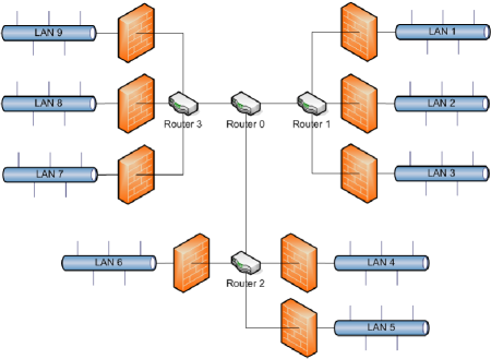
Figure 1: Sample computer network to be analyzed.

IV-A Simulation setup

Several attack types are simulated in Matlab on this network topology in order to compare the $H^{\infty}$-optimal controller with other controllers. As a simplification, a sub-network is assumed to be either infected or not infected. An infected sub-network sends malware to other sub-networks. Sub-networks become infected with some probability once they have received a certain threshold number of malware packets. This probability increases when higher thresholds are met. Clearly the propagation of these fictitious attacks is much simpler than that of an actual worm or virus, but it captures the underlying dynamics of an attack.

Four types of malware attacks are considered: no attack (A1); a high-traffic, slow spreading attack (A2); a low-traffic, slow-spreading attack (A3); and a low-traffic, fast-spreading attack (A4). In each of these attacks, one subnetwork is initially infected and sends malware to all other sub-networks.

Five response types are applied to each of these four attack types: no response (R1), the $H^{\infty}$-optimal controller response (R2), a threshold-based controller that implements a filter of some fixed magnitude when a certain amount of malicious packets are detected (R3), a controller that removes all suspicious packets ($\mathbf{y}(t)$) from each link (R4), and an optimal controller that minimizes the cost $\|\mathbf{z}\|^{2}$ (R5). For the linear quadratic Gaussian (LQG) optimization problem in (R5), which is obtained as the limit of the $H^{\infty}$ problem as $\gamma\rightarrow\infty$, we use the expected value of $\int^{\infty}_{-\infty}\|\mathbf{z}\|^{2}dt$ as the quadratic cost, which we again denote by $\|\mathbf{z}\|^{2}$ by a slight abuse of notation.

A few details relating to the numerical analysis of these controllers will now be given. The $A$ matrix is set to be the identity matrix multiplied by -1. Recall that this value quantifies the exponential decay of malicious packets on the link as they arrive at their destination sub-network. The $b$ quantity is set to 0.5. This value is consistent with a detection rate (true-positive rate) of 0.7 and a very low ($10^{-5}$) false-positive rate – a scenario considered in  [3]. The $D$ matrix is set up such that sub-networks are more likely to transfer the worm within their group of three sub-networks. The $C$ matrix is set to be 2 multiplied by the identity matrix, which is derived from values observed in the Ns-2 simulations to be explained in Section IV-C. It is assumed that $\mathbf{w}_{n}$ has a positive mean, as most malware detection schemes are set up to, if anything, overestimate the number of malicious packets. The standard deviation of $\mathbf{w}_{n}$ is relatively low. Also, the noise is assumed to be white Gaussian noise, although in reality this noise may well have some autocorrelation.

Simulations are run with three sets of cost functions ($\|z\|^{2}$ and $L$) that differ in their coefficients. The ratio between the cost on inbound malware packets $\mathbf{x}$ and the cost on filtering packets $\mathbf{u}$ (which involves a cost on filtering legitimate packets and also the filtering cost itself) is set at 10:1, 100:1, and 1000:1.

IV-B Matlab simulations

We first conduct a numerical analysis in Matlab. The simulations where no response is applied demonstrate that the assumed malware packet propagation rules mimic the “S-shaped” behavior of worm or virus propagation fairly well [2]. Note that in Fig. 2 the number of malware packets arriving at the two graphed sub-networks starts small when only one sub-network is initially infected. As the worm or virus spreads, the number of inbound malware packets increases rapidly for a period but eventually levels off when more and more sub-networks become infected.

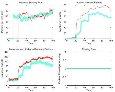
Figure 2: Numerical analysis of slow worm attack with no response applied on two (out of 9) sub-networks.

The $H^{\infty}$-optimal controller performs better than every other controller whenever malware is present, as seen in Table I. In this case, we choose a 100:1 malware packet to filtering action cost ratio. The resulting $\gamma^{*}$ is 4.52.

TABLE I: Cost Ratios ($L$) of Controllers Under Various Attacks ($b=0.5$)

Attack	R1	R2	R3	R4	R5
A1	0.00	3.48	0.00	2.35	2.04
A2	8.36	3.00	8.02	4.45	5.42
A3	9.07	2.88	5.76	4.42	4.71
A4	9.42	2.90	5.31	4.49	5.15

Table II shows the actual costs incurred by the system in each scenario with the same cost structure. The significantly lower cost values for the $H^{\infty}$-optimal controller in the face of attacks highlight its ability to filter enough to prevent sub-networks from becoming infected.

TABLE II: Costs ($\|z\|^{2}$) of Controllers Under Various Attacks ($b=0.5$) ($\times 10^{3}$)

Attack	R1	R2	R3	R4	R5
A1	0	1.172	0	0.788	0.682
A2	105.4	18.24	94.08	46.85	88.24
A3	22.68	5.579	16.77	12.50	10.34
A4	27.97	4.979	13.51	12.63	14.24

The preventative ability of the $H^{\infty}$-optimal controller can also be observed in Fig. 3. As soon as the first network detects an increase in inbound malware packets shortly after 10 time units, the controller begins filtering significantly (see Fig. 3 “Filtering Rate”) all across the network. This prevents the second sub-network from becoming infected. We indeed observe that it never sends malware packets in Fig. 3 “Malware Sending Rate.”

The ability of the centralized $H^{\infty}$-optimal controller to respond network-wide to an attack, and hence, increase filtering rates significantly even on sub-networks where there are not yet many malware packets being detected, provides an advantage over other controllers. Another advantage is that it tends to filter packets aggressively (see Fig. 3). We observe this robustness property of the $H^{\infty}$-optimal controller in the “Filtering Rate” graph of Fig. 3, where the number of packets filtered is higher than the number of inbound malware packets. This also contributes to preventing infections, decreasing cost to the network ($\|\mathbf{z}\|^{2}$), and to guaranteeing some level of performance ($\gamma$).

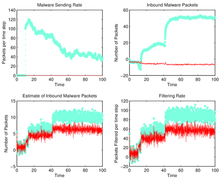
Figure 3: Numerical analysis of slow worm attack with $H^{\infty}$ response applied on two sub-networks.

For comparison, Fig. 4 shows the performance of the controller that removes all the estimated malware packets, thereby disregarding measurement errors and network-wide conditions. While it does over-filter, it does not filter network-wide when a single sub-network detects significant numbers of malware packets. Thus, the uninfected sub-network eventually becomes infected at around time step $25$, which causes it to send malware (Fig. 4). The LQR optimal controller (R5), on the other hand, does filter networkwide upon detection of inbound malware packets anywhere in the network. It does not, however, filter as much as the $H^{\infty}$-optimal controller. Moreover, it is hindered in that it assumes a zero-mean disturbance, an assumption that becomes more inaccurate as more sub-networks become infected.

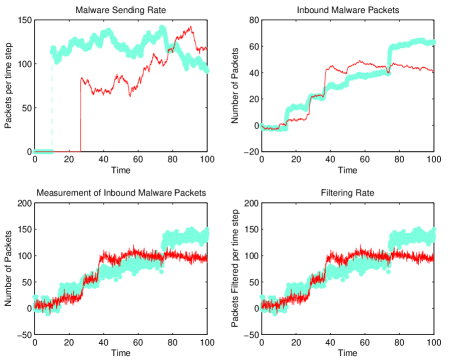
Figure 4: Numerical analysis of slow worm attack with the controller that removes as many malware packets as it measures on two sub-networks.

The $H^{\infty}$-optimal controller, on the other hand, tends to incur relatively high costs and cost ratios when there are no infected sub-networks due to its network-wide over-response (refer to Tables I and  II). The very characteristics that make it a strong controller in the face of attacks prove costly in the absence of attacks. In fact, the theoretical worst-case attack is actually quite small in magnitude and essentially maximizes $L$ by taking advantage of the tiny false alarms and corresponding excessive filtering that inaccurate measurements induce in the $H^{\infty}$-optimal controller. Figure 5 demonstrates this behavior. Note that the negative number of inbound malware packets indicates that all malware packets have been filtered and legitimate traffic is being removed from the link.

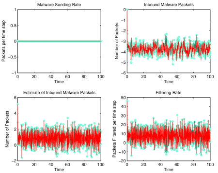
Figure 5: Network model response to no infections with the $H^{\infty}$-optimal controller.

Simulations were also run for other cost functions. The $H^{\infty}$-optimal controller performed relatively better when there was a greater cost put on the inbound malware packets and vice versa. This is to be expected, as this controller is rewarded more for being cautious when the inbound malware packets increase in cost. When the $b$ value was decreased from 0.5 to 0.3, the $H^{\infty}$-optimal controller also performs relatively better. This decrease in $b$ means that when filtering does occur, we are less likely to actually filter a malicious packet, and thus controllers that filter more are rewarded. A decreased $b$ could result from a lower true-positive rate, a higher false-positive rate, or a higher ratio of legitimate to malicious traffic.

IV-C Ns-2 Implementation

We simulate the traffic control algorithm developed at the packet level using the Ns-2 network simulator. Our goal is to further investigate the characteristics of the designed $H^{\infty}$-optimal controller and demonstrate its capabilities in a realistic setting. To enable comparisons with the numerical results obtained from Matlab simulations we define in Ns-2 the same network topology as in Section IV, which is depicted in Fig. 1. Depending on the specific application, the end nodes in this graph may represent a sub-network or any logical or physical set of hosts. As before, we assume high capacity links between nodes such that no malware packet is dropped due to congestion, corresponding to a worst-case scenario.

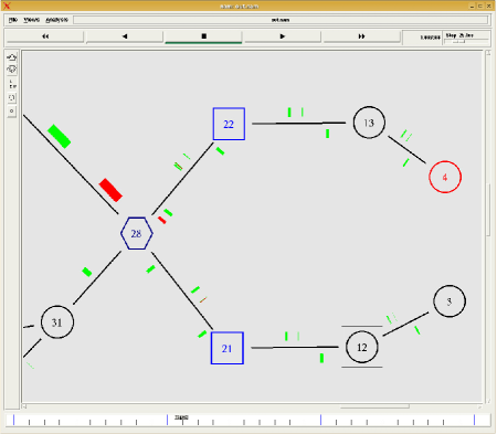
Figure 6: Screenshot of the Ns-2 simulator output. Green packets are legitimate and red packets are malware.

In order to simulate the filtering algorithm, we consider here a specific two-part implementation consisting of monitoring and filtering elements. The monitoring nodes, depicted as hexagons in Fig. 6, associate a malware score $s\in[0,99]$ to each individual packet passing through the link from the outside. As a simplification, we simulate only inbound monitoring and filtering. However, a symmetrical outbound counterpart of the scheme can easily be implemented. The monitoring elements use this score $s$ and a specific constant threshold to make an initial estimate on the nature of the packet and label it as malware or not. A count of these observed malware packets gives $\mathbf{y}(t)$. The monitoring node may utilize any set of algorithms or approaches to determine this quantity. We generate the scores randomly according to different probability distributions for legitimate and malicious packets and use a fixed threshold to simulate this process. This method is similar in some ways to the scoring strategy proposed in  [9].

The filtering elements depicted as boxes in Fig. 6 first fetch the malware score $s$ and the flag from the headers of inbound packets, and then use either a heuristic or a $H^{\infty}$ controller-based algorithm to make filtering decisions. In this implementation, the algorithms decide on a time-varying threshold value (different than the previous constant measurement threshold), resulting in a dynamic filtering scheme. The packets with a score higher than the threshold are filtered. For comparison purposes, we simulate the R4 algorithm in Section IV-A, which we denote as heuristic, in addition to the $H^{\infty}$ algorithm. We do not simulate any filtering scheme with a time-invariant threshold as it clearly would under perform in a dynamic network environment when compared with the dynamic threshold algorithms.

We calculate the $H^{\infty}$-optimal controller offline in Matlab and transfer the results to the Ns-2 simulator. In accordance with the model in Section II, the resulting controller decides on the number of malware packets to be filtered at a given time interval. We translate this number into a threshold value by periodically observing the distribution of scores generated by the monitoring element. Hence, the threshold is chosen such that the number of packets with a score higher than the threshold (i.e., to be filtered) matches the number dictated by the $H^{\infty}$-optimal controller.

Remark IV.1.

It is important to note that the example Ns-2 implementation we choose here does not play a significant role for the analysis and demonstration of our algorithm. In fact, depending on the specific application at hand, one can choose a variety of equivalent implementations without loss of any generality. For example, the monitoring and filtering elements can be parts of larger units each or combined within a dedicated physical device. Or the monitoring element can be deployed as a dedicated hardware device and the filtering element as part of a firewall implementation. Clearly, the possible combinations are numerous.

We simulate, compare, and contrast the $H^{\infty}$ and detection-based heuristic filtering schemes in a variety of scenarios under different cost structures, detection capabilities, and traffic levels. The hypothetical scenarios we consider are summarized as follows:

1. A cost on malware packets ($\mathbf{x}$) to cost on filtering ($\mathbf{u}$) ratio of 100:1 in $\|\mathbf{z}\|^{2}$ and $L$. We assume that the monitoring devices are capable of scoring and labeling only half of the malware packets correctly (S1).

2. The cost is the same as in Scenario 1, but we consider a more pessimistic case where the monitoring device only detects a quarter of the total malware packets (S2).

3. This scenario is the same as Scenario 1 except for an increase in the cost coefficient ratio to 200:1 (S3).

4. Likewise, this scenario is the same as Scenario 2 with a cost coefficient ratio of 200:1 (S4).

5. The final scenario matches Scenario 1 but has a cost coefficient ratio of 0.1:1 (S5).

In all of the above cases, each end-node (sub-network) sends randomly fluctuating $1000$-KB legitimate traffic to all sub-networks. In addition we consider an “infection” or worm-like malware propagation scheme, where each sub-network becomes “infected” with some probability if it receives sufficiently many malware packets and afterward generates malware traffic of $200$-KB to other nodes.

TABLE III: Cost Results of Ns-2 Simulations

	$H^{\infty}$-Optimal			Detection-Based
Scen.	$L$	$\|\mathbf{z}\|^{2}$   ($\times 10^{6}$)	$\gamma^{*}$	$L$	$\|\mathbf{z}\|^{2}$   ($\times 10^{6}$)
S1	3.9	77	3.2	4.9	147
S2	3.7	89	3.2	6.6	369
S3	4.2	87	4.2	6.9	287
S4	4.9	155	4.2	9.3	736
S5	0.31	0.68	0.3	1.05	6.78

The numerical results for both of the algorithms under each scenario described above are summarized in Table III. We observe here several expected characteristics of the $H^{\infty}$ controller such as optimality with respect to the cost functions and robustness. In almost all of the cases and over a wide range of cost coefficient ratios it outperforms the detection-based heuristic scheme. More importantly, it exhibits robustness with respect to variations in detection quality (see case 1 versus 2) and guarantees an upper bound on the cost $L$. It is observed that the $L$ value is always near the theoretically calculated bound $\gamma^{*}$. Another indication of the $H^{\infty}$-optimal controller’s robustness is the satisfactory performance of the controller even though it is calculated offline with estimated system characteristics. This, along with the assumptions inherent in the model, explains the occasional discrepancies observed between $L$ values and the theoretical upper-bounds $\gamma^{*}$.

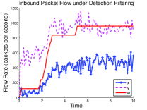
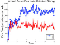
Figure 7: Various inbound packet flow rates to sub-network 1 under the detection-based filtering.

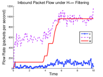
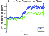
Figure 8: Various inbound packet flow rates to sub-network 1 under $H^{\infty}$ controller.

We next analyze the time-series data collected for a representative sub-network. We depict various quantities of interest $x$ (malware packets that pass through the filter), $y$ (packets labeled as malware by monitor), and $u$ (filtering rate) as in Sub-section IV-B. In addition, we plot the the rate of falsely positive labeled packets $m$ and the rate of real malware flow, $w$. Figure 7 shows the evolution of these quantities over time in Scenario 1 under the detection-based scheme, whereas Fig. 8 depicts the counterpart for the $H^{\infty}$ controller. We observe that the $H^{\infty}$ controller performs better than the detection-based scheme in terms of removing the malware packets through aggressive filtering in line with the preferences expressed in the cost function. Concurrently, this leads to a slower infection rate as can be inferred from the evolution of real malware flow rate ($w$) in Fig. 8. On the other hand, when the cost coefficient ratio changes to the one in Scenario 5, $H^{\infty}$ controller is much less aggressive in filtering due to high cost of dropping legitimate packets. This can be seen in Fig. 9, where the maximum filtering rate is significantly lower that in other scenarios.

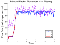
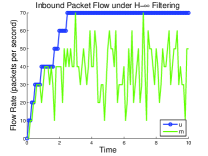
Figure 9: Various inbound packet flow rates to sub-network 1 under $H^{\infty}$ controller when the cost coefficient ratio is $0.1:1$ (Scenario 5).

We finally consider the case when one of the sub-networks (say $5$) is more valuable than others and needs more intensive inbound filtering. This preference can easily be reflected to the cost function by increasing the respective entry of the matrix $H$ in (4). Thus, the $H^{\infty}$ controller reacts accordingly and filters more aggressively for this sub-network compared to any other as depicted in Fig. 10.

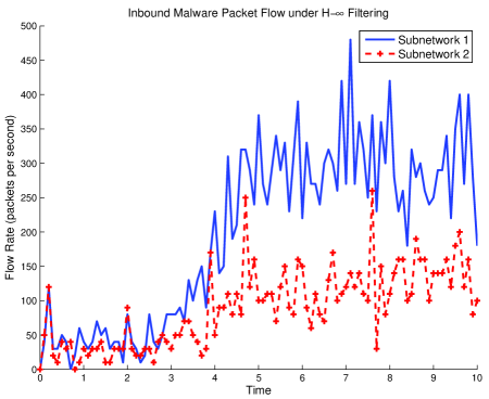
Figure 10: Inbound malware packet flow rates to sub-networks 1 and 5 (more valuable) under $H^{\infty}$ controller.

V Conclusion

We have studied an application of robust control theory to network security by investigating an $H^{\infty}$-optimal control formulation of the network filtering problem that captures its inherent challenges such as the base-rate fallacy and takes into account relevant costs. The corresponding $H^{\infty}$-optimal controller has been derived and analyzed numerically in Matlab as well as simulated in Ns-2. The controller performs better than alternative controllers when there is a significant amount of malware traffic present. In addition, it provides a certain performance guarantee for a wide range of conditions.

There exist several possible extensions to this work. Obtaining a distributed version of this controller for a larger system could be one future direction. Another research direction is the application of similar $H^{\infty}$-optimal controllers to other network security problems, such as spam filtering and DDoS attacks.

References

- [1] D. Moore, V. Paxson, S. Savage, C. Shannon, S. Staniford, and N. Weaver, “Inside the slammer worm,” IEEE Security & Privacy Magazine, vol. 1, pp. 33–39, July-Aug. 2003.
- [2] D. Moore, C. Shannon, and K. Claffy, “Code-red: A case study on the spread and victims of an internet worm,” in Proc. of ACM SIGCOMM Workshop on Internet Measurement, Marseille, France, 2002, pp. 273–284.
- [3] S. Axelsson, “The base-rate fallacy and its implications for the difficulty of intrusion detection,” in Proc. of 6th ACM Conference on Computer and Communications Security, Kent Ridge Digital Labs, Singapore, 1999, pp. 1–7.
- [4] K. Rohloff and T. Başar, “The detection of RCS worm epidemics,” in Proc. of ACM Workshop on Rapid Malcode, Fairfax, VA, 2005, pp. 81–86.
-
[5]
Cisco, “NAT and stateful inspection in Cisco IOS firewall,” white
paper, 2006. [Online]. Available:
http://www.cisco.com/en/US/tech/tk648/tk361/technologies_white_paper
09186a0080194af8.shtml - [6] T. Başar and P. Bernhard, H∞-Optimal Control and Related Minimax Design Problems: A Dynamic Game Approach, 2nd ed. Boston, MA: Birkhäuser, 1995.
- [7] M. Tulloch, Microsoft Encyclopedia of Security. Redmond, WA: Microsoft Press, 2003.
- [8] S. Hazelhurst, “A proposal for dynamic access lists for TCP/IP packet filtering,” in Proc. of South African Instutute of Computer Scientists and Information Technologists Annual Conference, Pretoria, South Africa, September 2001, http://arxiv.org/abs/cs/0110013.
- [9] Y. Kim, W. C. Lau, M. C. Chuah, , and H. J. Chao, “Packetscore: A statistics-based packet filtering scheme against distributed denial-of-service attacks,” IEEE Trans. on Dependable and Secure Computing, vol. 3, no. 2, pp. 141–155, April-June 2006.
- [10] C. Zou, D. Towsley, and W. Gong, “A firewall network system for worm defense in enterprise networks,” University of Massechusetts, Amherst, MA, Technical Report TR-04-CSE-01, Feb. 2004.
- [11] T. M. Chen and N. Jamil, “Effectiveness of quarantine in worm epidemics,” in Proc. of IEEE ICC 2006, Istanbul, Turkey, June 2006, pp. 2142–2147.
- [12] T. Alpcan and T. Başar, “A game theoretic analysis of intrusion detection in access control systems,” in Proc. 43rd IEEE Conf. Decision and Control, Paradise Island, Bahamas, December 2004, pp. 1568–1573.