Uncovering the community structure associated with the diffusion dynamics on networks

Abstract

As two main focuses of the study of complex networks, the community structure and the dynamics on networks have both attracted much attention in various scientific fields. However, it is still an open question how the community structure is associated with the dynamics on complex networks. In this paper, through investigating the diffusion process taking place on networks, we demonstrate that the intrinsic community structure of networks can be revealed by the stable local equilibrium states of the diffusion process. Furthermore, we show that such community structure can be directly identified through the optimization of the conductance of network, which measures how easily the diffusion occurs among different communities. Tests on benchmark networks indicate that the conductance optimization method significantly outperforms the modularity optimization methods at identifying the community structure of networks. Applications on real world networks also demonstrate the effectiveness of the conductance optimization method. This work provides insights into the multiple topological scales of complex networks, and the obtained community structure can naturally reflect the diffusion capability of the underlying network.

As two main focuses of the study of complex networks, the community structure and the dynamics on networks have both attracted much attention in various scientific fields. On one hand, many methods for community detection have been proposed and applied successfully to some specific complex networks [1, 2, 3, 4, 5, 6, 7, 8, 9]. Each method requires, explicitly or implicitly, a definition of a community from different perspectives, such as the centrality measures, link density, percolation theory, and network compression. Generally, community structure is known as the existence of groups of nodes such that nodes within a group are much more connected to each other than to the rest of the network [10]. Community structure may provide insight into the relation between the structure and the function of complex networks. Taking the World Wide Web as an example, closely hyperlinked web pages form a community and they often concern related topics [11, 12].

A well known definition for a community is via the modularity, which is proposed by Newman et al as a quality function for a partition of the network. Modularity is effective for detecting the community structure of many real world networks. However, as pointed out by Fortunato et al [13], modularity suffers the resolution limit problem and this problem raises concerns about the reliability of the communities detected through the optimization of modularity. In [14], the authors claimed that the resolution limit problem is attributable to the coexistence of multiple scale descriptions of the topological structure of the network, while only one scale is obtained through directly optimizing the modularity. In addition, the definition of modularity only considers the significance of link density from the static topological structure of network, and it is unclear how the modularity based community structure is correlated to the dynamics on network.

On the other hand, many efforts are devoted to understanding the properties of the dynamical processes taking place on the underlying networks [15, 16]. In recent years, researchers have begun to investigate the correlation between the community structure and the dynamics on networks. For example, Arenas et al pointed out that the synchronization reveals the topological scale in complex networks [17]. In addition, the random walk on a network was also extensively studied and used to uncover community structure of the network [18, 19, 20]. In [21, 22], the random walk on a network is introduced for defining the distance between network nodes, and an algorithm based on this distance is proposed for partitioning the network into communities. In [23], the authors proposed quantifying and ranking the quality of network partitions in terms of their stability, defined as the clustered autocovariance in the random walk process taking place on the network.

In this paper, through investigating the diffusion process taking place on the network, we note that local equilibrium states appear before the diffusion process reaches the final equilibrium state. The stability of local equilibrium states can be measured by their duration time in the diffusion process. Then, we demonstrate that the intrinsic community structure is revealed by the stable local equilibrium states of the diffusion process. Furthermore, we show that such community structure can be directly identified through the optimization of the conductance of the network, which measures how easily the diffusion among different communities occurs.

We first introduce some notations used later. An undirected network $G=(V,E)$ with $N$ nodes is often described in terms of its adjacency matrix $A$ whose elements $A_{xy}$ denote the strength of the link connecting the nodes $x$ and $y$. The strength of node $x$ is denoted by $s_{x}=\sum_{y}{A_{xy}}$. For a node set $V_{1}\subseteq V$, $|V_{1}|$ denotes the number of node in $V_{1}$, the volume of $V_{1}$ is defined as $vol(V_{1})=\sum_{x\in V_{1}}s_{x}$, and $in\_vol(V_{1})=\sum_{x\in V_{1},y\in V_{1}}{A_{xy}}$ is referred to as the inward volume of $V_{1}$.

We start with investigating the diffusion process which describes the dynamics of a random walker moving on the network. At each time $t$, the random walker moves from its current node $x$ to one of its neighboring nodes $y$ randomly with the probability $p(x\rightarrow y)=A_{xy}/s_{x}$. The dynamics of this process can be described as

$$\frac{d\rho_{x}(t)}{dt}=-r\sum_{y}L^{T}_{xy}\rho_{y}(t)\,,\ \ x=1,\ldots,N\,,$$ (1)

where $\rho_{x}(t)$ is the probability that the random walker resides at the node $x$ at the time $t$, and $r$ is a parameter controlling the rate of the diffusion process. The matrix $L$ is the normalized Laplacian matrix defined as $L=I-D^{-1}A$, where $I$ is the identity matrix and $D$ is a diagonal matrix with its diagonal elements $D_{xx}=s_{x}$.

For any starting node, as time proceeds, the diffusion process described in the equation (1) will definitely move towards equilibrium if the underlying undirected network is connected and non-bipartite [24]. When the diffusion process is at the equilibrium state, it satisfies the so-called detailed balance condition [25], i.e., the probability that the random walker walks through the nodes $x$ and $y$ successively is equal to the probability that the random walker walks through the nodes $y$ and $x$ successively. Formally, the detailed balance condition can be denoted by $\rho_{x}(t)p(x\rightarrow y)=\rho_{y}(t)p(y\rightarrow x)$ and the reduced form is $\rho_{x}(t)/s_{x}=\rho_{y}(t)/s_{y}$ for undirected networks.

We explore the transients in the whole diffusion process instead of only the final equilibrium state. During the diffusion process on a network, it is known that the detailed balance condition is satisfied among highly interconnected nodes first and then, sequentially, among less interconnected ones, until among all the nodes. In order to evaluate how closely two nodes $x$ and $y$ satisfy the detailed balance condition at the time $t$, we introduce a measure $c_{xy}(t)$ as

$$c_{xy}(t)=\left\langle\left|\frac{\rho_{x}(t)}{s_{x}}-\frac{\rho_{y}(t)}{s_{y}}\right|\right\rangle,$$ (2)

where $\langle\cdots\rangle$ averages over different realizations of the diffusion process with randomly selected starting nodes. In practice, a pair of nodes $x$ and $y$ is said to satisfy the detailed balance condition at the time $t$ when $c_{xy}(t)$ is smaller than a given threshold. A set $V$ of nodes is said to satisfy the detailed balance condition if the average value $\sum_{y\in V}{c_{xy}(t)}/|V|$ of $c_{xy}(t)$ for each node $x$ is smaller than the given threshold. Relative to the final equilibrium state, we say that the diffusion process is at a local equilibrium state when only several groups of nodes locally satisfy the detailed balance condition. Using the matrix $c_{xy}(t)$, we can trace the different local equilibrium states during the diffusion process.

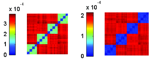
Figure 1: (color online). The matrix $c_{xy}(t)$ of two transients in the diffusion process taking place on the H13-4 network. Each value of $c_{xy}(t)$ is the average over $10,000$ realizations of the diffusion process with randomly selected starting nodes. The parameter $r=0.01$.

As an example, we use $c_{xy}(t)$ to analyze the diffusion process on the H13-4 network, which is constructed according to [17]. The network has two predefined hierarchical levels, the first hierarchical level consists of $4$ groups of $64$ nodes and the second hierarchical level consists of $16$ groups of $16$ nodes. Figure 1 illustrates the $c_{xy}(t)$ of two transients corresponding to two different local equilibrium states of the diffusion process. The squares along the diagonal suggest that the corresponding groups of nodes satisfy the detailed balance condition. These node groups reveal the predefined hierarchical levels in the H13-4 network. For comparison, we further investigate the diffusion dynamics on the randomized H13-4 network, which is constructed through shuffling the edges of the H13-4 network used in figure 1. From figure 2(a), we can see that there is no node group locally satisfying the detailed balance.

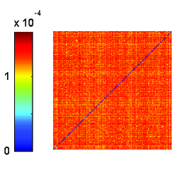
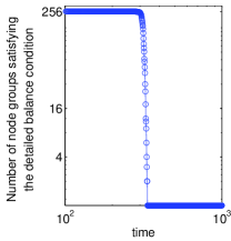
(a)                                      (b)

Figure 2: (color online). The diffusion dynamics on the randomized H13-4 network. (a) The matrix $c_{xy}(t)$ of a transient in the diffusion process. Each value of $c_{xy}(t)$ is the average over $10,000$ realizations of the diffusion process with randomly selected starting nodes. The parameter $r=0.01$. (b) The number of node groups satisfying the detailed balance condition as a function of time $t$. Here, the threshold for $c_{xy}(t)$ is set to be $1.0\times 10^{-4}$.

A phenomenon similar to that illustrated in figure 1 has also been observed in the synchronization process. In [17], the authors claimed that this phenomenon reveals the topological scale of networks. The authors also pointed out that the phenomenon of the synchronization process is correlated with the spectrum of the Laplacian matrix associated with the underlying network. According to the characteristics of the Laplacian matrix, as pointed out in [26], the community structure revealed by the synchronization process is heavily affected by the heterogeneous degree distribution and the community size distribution. In the following, we will show that the local equilibrium state phenomenon is correlated with the spectrum of the normalized Laplacian matrix, which takes the heterogeneous degree and community size distribution into account and thus behaves better than the Laplacian matrix as regards clustering the nodes of network [26].

In this paper, a local equilibrium state is regarded as stable if the set of node groups satisfying the detailed balance condition remains unchanged for a long duration in the diffusion process. To investigate the stability of the local equilibrium states, we study the solution of equation (1) in terms of the normal modes $\varphi_{i}(t)$, which reads

$$\rho_{x}(t)=\sum_{i}{U_{xi}\varphi_{i}(t)}=\sum_{i}{U_{xi}\varphi_{i}(0)e^{-\lambda_{i}rt}}\,,\ \ x=1,\ldots,N\,,$$ (3)

where the $\lambda_{i}$ are the eigenvalues of the transpose of the normalized Laplacian matrix $L$, and $U$ is the eigenvector matrix whose $i$th column is the eigenvector $u_{i}$ corresponding to the eigenvalue $\lambda_{i}$. Given the starting node of the diffusion process, the initial amplitudes $\varphi_{i}(0)$ can be determined according to equation (3) due to the eigenvector matrix $U$ being fixed, i.e., $\varphi_{i}(0)$ only depends on the starting node of the diffusion process. Note that, as pointed out following the equation (2), we investigate the average behavior of many different diffusion processes with randomly selected starting nodes. Thus, the choice of the starting nodes does not affect the results of the following analysis in this paper. Without loss of generality, we rank these eigenvalues in the ascending order $0=\lambda_{1}\leq$$\lambda_{2}\leq$$\cdots\leq$$\lambda_{i}\leq$$\dots$ $\leq\lambda_{N}$.

As time proceeds in the diffusion process, these normal modes $\varphi_{i}(t)=\varphi_{i}(0)e^{-\lambda_{i}rt}(i\neq 1)$ will decay to zero. We use $\tau_{i}$ to denote the time when the normal mode $\varphi_{i}(t)$ decays to zero. Formally, $\tau_{i}$ is infinite. In practice, a threshold $\varepsilon$ is usually used to determine when $\varphi_{i}(t)$ decays to zero, i.e., $\varphi_{i}(t)<\varepsilon$. In this case, we have

$$\tau_{i}=\frac{1}{\lambda_{i}}\times\frac{ln\varphi_{i}(0)-ln\varepsilon}{r}.$$ (4)

All these moments $\tau_{i}$ ($1\leq i\leq N$) form a series of time intervals, respectively $[\tau_{N+1}=0,\tau_{N})$, $[\tau_{N},\tau_{N-1})$, $\cdots$, $[\tau_{i+1},\tau_{i})$, $\cdots$, $[\tau_{3},\tau_{2})$, $[\tau_{2},\tau_{1}=\infty)$. These time intervals divide the whole diffusion process into $N$ stages. Specifically, the time interval $[\tau_{i+1},\tau_{i})$ is regarded as the $i$th stage. When the diffusion process is at the $i$th stage, only the normal modes $\varphi_{j}(t)$($1\leq j\leq i$) have not decayed to zero. Thus we have

$$\rho_{x}(t)\approx\sum_{j=1}^{i}{U_{xj}\varphi_{j}(t)}\,,\ \ x=1,\ldots,N\,.$$ (5)

This indicates that the value $\rho_{x}(t)$ of node $x$ at the $i$th stage can be represented by the $i$-dimension coefficient vector of $\varphi_{j}(t)$, i.e., $(U_{x1},U_{x2},\cdots,U_{xj},\cdots,U_{xi})$. According to equations (2) and (5), given a threshold, we can identify the node groups satisfying the detailed balance condition through clustering the normalized $i$-dimension vectors of $(U_{x1},U_{x2},\cdots,U_{xj},\cdots,U_{xi})$ using, for example, the $k$-means clustering method. The set of such node groups is unchanged due to the non-decayed normal modes being fixed during the same stage. This means that the local equilibrium state is stable if the corresponding stage persists for a long time.

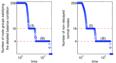
Figure 3: (color online). Left: the number of node groups satisfying the detailed balance condition as a function of time $t$. Here, the threshold for $c_{xy}(t)$ is set to be $1.0\times 10^{-4}$. Right: the number of non-decayed normal modes in terms of the time $t$.

Taking the H13-4 network as an example, the left panel of figure 3 shows the different local equilibrium states of the diffusion process and the right panel illustrates the different stages in terms of the number of non-decayed normal modes of the diffusion process. Through comparing the two panels, we see that each time one normal mode decays to zero, the diffusion process changes from a local equilibrium state to a new one. It is observed that two stable local equilibrium states with long durations emerge in the diffusion process. The node groups corresponding to these two states clearly reveal the intrinsic community structure of the H13-4 network. In addition, from figure 2(b), we can see that no stable local equilibrium state appears in the diffusion process taking place on the randomized H13-4 network. This is reasonable, as it is commonly believed that randomized network have no community structure. All these findings suggest that the appearance of stable local equilibrium states in a diffusion process indicates the existence of community structure in the underlying network.

Note that the diffusion occurs much more frequently within the node groups than among them when the diffusion process is at a stable local equilibrium state. This indicates that there exists a high transitive cohesion inside such node groups. The community structure comprised of these node groups could well reflect the diffusion dynamics on the underlying network. Regarding such community structure as a partition of a network, we measure the quality of the partition through introducing the conductance of networks, which reflects how easily the diffusion occurs among different communities.

For a given partition $\mathcal{P}=\{V_{1},\ldots,V_{k}\}$, the conductance is defined as the average departure probability, $p_{dept}(V_{i})$, of all the communities $V_{i}$, that is $C(\mathcal{P})=\frac{1}{k}\sum_{i=1}^{k}{p_{dept}(V_{i})}$. The departure probability of a community $V_{i}$ is the probability that the random walker departs from $V_{i}$ in the next time step given that it resides at $V_{i}$ when the diffusion process is at the final equilibrium state. Formally, the departure probability of $V_{i}$ can be computed by using

$$p_{dept}(V_{i})=\frac{\sum_{x\in V_{i},y\in\overline{V}_{i}}{\rho_{x}(\infty)p(x\rightarrow y)}}{\sum_{x\in V_{i}}{\rho_{x}(\infty)}}=1-\frac{in\_vol(V_{i})}{vol(V_{i})},$$ (6)

where $\rho_{x}(\infty)=s_{x}/vol(V)$ is the stationary distribution which characterizes the final equilibrium state of the diffusion process. In this way, the conductance is formally denoted by

$$C(\mathcal{P})=\frac{1}{k}\sum_{i=1}^{k}{\left(1-\frac{in\_vol(V_{i})}{vol(V_{i})}\right)}.$$ (7)

Actually, it can be proved that the community structure associated with the stable local equilibrium state can be exactly identified through minimizing the conductance directly. Without loss of generality, we assume that the stable local equilibrium state emerges at the $k$th stage in the diffusion process. As mentioned above, the community structure associated with this state can be identified through clustering the normalized $k$-dimension vectors of $(U_{x1},U_{x2},\cdots,U_{xi},\cdots,U_{xk})$. Further, through the matrix trace maximization method [27], it can be proved that the optimization of the conductance for a fixed $k$ can be done through clustering the top $k$ eigenvectors of the transpose of the normalized Laplacian matrix, corresponding to the $1$st to $k$th columns of $U$. Therefore, the optimization of conductance provides an effective way to identify the community structure associated with the stable local equilibrium state.

Now we clarify the difference between the conductance used in this paper and the earlier measure for the quality of network partition from the perspective of a random walk on networks. Firstly, as pointed out in [28], as a measure of the quality of network partition, the modularity can be described as the difference between the probability that a random walker resides in the same community on two successive time steps and the probability that two independent random walkers both resides in the same community. Secondly, in [23], through considering the random path with length $t$ instead of the length $1$ for the modularity and the length of infinity for the spectral partition, the authors proposed that the stability of network partitions be defined as the clustered autocovariance of the random walk. This stability provides a general framework for quantifying and ranking the quality of network partitions from the perspective of the whole network, i.e., it characterizes the fraction of the within-community random paths with length $t$ with respect to all the random paths of length $t$. However, the conductance considers the quality of network partition from the perspective of each community instead of the whole network, i.e., it reflects the fraction of within-community random paths with respect to all the random paths departing solely from the community considered. This provides the advantage for handling the heterogeneous distribution of community size (or volume) which is common to real world networks. As follows, the application of the conductance optimization method to the benchmarks of Lancichinetti et al also demonstrates that our method can effectively handle the heterogeneous distribution of community size.

To test the effectiveness of our method for community detection based on the optimization of conductance, we utilize the benchmark proposed by Lancichinetti et al in [29]. This benchmark provides networks with heterogeneous distributions of node degree and community size. Thus it poses a much more severe test of community detection algorithms than standard benchmarks. Many parameters are used to control the generated networks in this benchmark: the number of nodes $N$, the average node degree $\langle k\rangle$, the maximum node degree max$\rule[-1.0pt]{4.26773pt}{0.3pt}k$, the mixing ratio $\mu$, the exponent of the power law node degree distribution $t_{1}$, the exponent of the power law distribution of community size $t_{2}$, the minimum community size min$\rule[-1.0pt]{4.26773pt}{0.3pt}c$, and the maximum community size max$\rule[-1.0pt]{4.26773pt}{0.3pt}c$. In our tests, we use the default parameter configuration where $N=1000$, $\langle k\rangle=15$, max$\rule[-1.0pt]{4.26773pt}{0.3pt}k=50$, $t_{1}=2$, $t_{2}=1$, min$\rule[-1.0pt]{4.26773pt}{0.3pt}c=20$, and max$\rule[-1.0pt]{4.26773pt}{0.3pt}c=50$. By tuning the parameter $\mu$, we test the effectiveness of our method on the networks with different fuzziness of communities. The larger the parameter $\mu$, the fuzzier the community structure of the generated network. In addition, we adopt the normalized mutual information (NMI) [30] in order to compare the partition found by the algorithms with the answer partition. The larger the NMI, the more effective the tested algorithm.

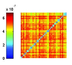
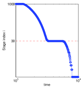
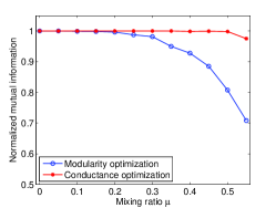
(a)                                (b)                                (c)

Figure 4: (color online). (a-b) The most stable local equilibrium and the different stages of the diffusion process on the benchmark network with the mixing ratio $\mu$=$0.3$ and the number of communities is $30$. (c)Comparison between the conductance optimization method and the modularity optimization method on benchmark networks. Each point corresponds to an average over $100$ network realizations.

Figure 4(a-b) illustrate the most stable local equilibrium state and the different stages of the diffusion process on the benchmark network with the mixing ratio $\mu$=$0.3$ and the number of communities equal to $30$. The squares along the diagonal indicate the predefined communities in the network. The number of these communities is clearly revealed by the most stable local equilibrium state. Figure 4(c) shows the comparison between the conductance optimization method and the modularity optimization method in terms of the NMI on the benchmark network. When the community structure is evident, both our method and the modularity optimization method (e.g., the fast unfolding algorithm [7] and the spectral method [3]) can accurately identify the community structure. However, when the community structure becomes fuzzier, the performance of the modularity optimization method deteriorates while our method still achieves rather good results.

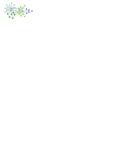
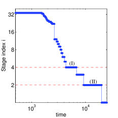
(a)                                                           (b)

Figure 5: (color online). Illustration of the conductance optimization method using the real world network. (a) The friendship network of the karate club studied by Zachary [1]. Colors are used to differentiate the communities uncovered by the conductance optimization method when considering the stage (I) in figure 5(b). Shapes, circle and square, are used to distinguish the communities corresponding to the stage (II) and the real social split of this network observed by Zachary. (b) The different stages of the diffusion process taking place on the network in figure 5(a). Two most stable equilibrium states are marked with (I) and (II).

In addition, we also tested the conductance optimization method on many real world networks which are widely used to evaluate community detection methods. These networks include the social network of Zachary’s karate club, the social network of dolphins of Lusseau et al, the college football network of the United States [10], the journal index network constructed in [5], and the network of political books [3]. For all these networks, the conductance optimization method obtains extremely good results. Taking Zachary’s network as an example, figure 5(b) illustrates the different stages of the diffusion process taking place on the network. The two most stable local equilibrium states are marked (I) and (II), and the corresponding communities are depicted in figure 5(a). Besides the stages (I) and (II), another relatively stable state can be also observed during the diffusion process, as shown in figure 5(b). The corresponding three communities are respectively the one comprised of all the circle nodes and two communities formed by the square nodes but with different colors, as shown in figure 5(a). Actually, as regards the three stable states, it is really hard to say which the best one is. In this paper, the duration time of each state may provide an effective candidate measure for the significance of network divisions.

In summary, we find that several stable local equilibrium states emerge during the diffusion process on networks with community structure. These stable states reveal the intrinsic community structure of the underlying networks. We further propose a conductance optimization method to identify the community structure, which naturally reflects the diffusion capability of the network. This work provides new insights into the number of communities and the multiple topological scales of complex network. As future work, we will study the relation and difference between the conductance and the modularity method.

References

References

- [1] M. E. J. Newman and M. Girvan, Phys. Rev. E 69, 026113 (2004).
- [2] R. Guimerà and L. A. N. Amaral, Nature(London) 433, 895 (2005).
- [3] M. E. J. Newman, Proc. Natl. Acad. Sci. U.S.A. 103, 8577 (2006).
- [4] G. Palla, I. Derényi, I. Farkas, and T. Vicsek, Nature(London) 435, 814 (2005).
- [5] M. Rosvall and C. T. Bergstrom, Proc. Natl. Acad. Sci. U.S.A. 104, 7327 (2007).
- [6] H. W. Shen, X. Q. Cheng, K. Cai and M. B. Hu, Physica A 388, 1706 (2009).
- [7] V. D. Blondel, J.-L. Guillaume, R. Lambiotte and E. Lefebvre, J. Stat. Mech.: Theory and Exp., (2008) P10008.
- [8] H. W. Shen, X. Q. Cheng, and J. F. Guo, J. Stat. Mech.: Theory and Exp., (2009) P07042.
- [9] S. Fortunato, Phys. Rep. 486, 75-174 (2010).
- [10] M. Girvan and M. E. J. Newman, Proc. Natl. Acad. Sci. U.S.A. 99, 7821 (2002).
- [11] J. Kleinberg and S. Lawrence, Science 294, 1849 (2001).
- [12] X. Q. Cheng, F. X. Ren, S. Zhou and M. B. Hu, New J. Phys. 11, 033019 (2009).
- [13] S. Fortunato and M. Barthélemy, Proc. Natl. Acad. Sci. U.S.A. 104, 36 (2007).
- [14] A. Arenas, A. Fernández and S. Gómez, New. J. Phys. 10, 053039 (2008).
- [15] S. Boccaletti, V. Latora, Y. Moreno, M. Chavez, and D. -U. Hwang, Phys. Rep. 424, 175 (2006).
- [16] A. Arenas, A. Dìaz-Guilera, J. Kurths, Y. Moreno, and C. Zhou, Phys. Rep. 469, 93 (2008).
- [17] A. Arenas, A. Dìaz-Guilera, C. J. Perez-Vicente, Phys. Rev. Lett. 96, 114102, (2006).
- [18] M. Rosvall and C. T. Bergstrom, Proc. Natl. Acad. Sci. U.S.A. 105, 1118 (2008).
- [19] H. Zhou and R. Lipowsky, Lecture Notes in Computer Science 3038, 1062 (2004).
- [20] P. Pons and M. Latapy, Lecture Notes in Computer Science 3733, 284 (2005).
- [21] H. Zhou, Phys. Rev. E 67, 041908 (2003).
- [22] H. Zhou, Phys. Rev. E 67, 061901 (2003).
- [23] J.-C. Delvene, S. N. Yaliraki, and M. Barahona, arXiv:0812.1811.
- [24] J. D. Noh and H. Rieger, Phys. Rev. Lett. 92, 118701, (2004).
- [25] A. Barrat, M. Barthélemy, and A. Vespignani, Dynamical Processes on Complex Networks (Cambridge University Press, Cambridge, UK) (2008).
- [26] U. von Luxburg, Stat. Comput. 17, 395 (2008).
- [27] S. X. Yu and J. Shi, in Proceedings of the Ninth IEEE International Conference on Computer Vision (IEEE Computer Society, Washington DC, 2003), pp. 313–319.
- [28] T. S. Evans and R. Lambiotte, Phys. Rev. E 80, 016105 (2009).
- [29] A. Lancichinetti, S. Fortunato, and F. Radicchi, Phys. Rev. E 78, 046110 (2008).
- [30] L. Danon, J. Duch, A. Dìaz-Guilera, J. Duch and A. Arenas, J. Stat. Mech., P09008 (2005).