14

12

Detecting the orientation of magnetic fields in galaxy clusters

Christoph Pfrommer¹, L. Jonathan Dursi^2,1

¹Canadian Institute for Theoretical Astrophysics, University of Toronto, Toronto, Ontario, M5S 3H8, Canada
²SciNet Consortium, University of Toronto, Toronto, Ontario, M5T 1W5, Canada

Clusters of galaxies, filled with hot magnetized plasma, are the largest bound objects in existence and an important touchstone in understanding the formation of structures in our Universe. In such clusters, thermal conduction follows field lines, so magnetic fields strongly shape the cluster’s thermal history; that some have not since cooled and collapsed is a mystery. In a seemingly unrelated puzzle, recent observations of Virgo cluster spiral galaxies imply ridges of strong, coherent magnetic fields offset from their centre. Here we demonstrate, using three-dimensional magnetohydrodynamical simulations, that such ridges are easily explained by galaxies sweeping up field lines as they orbit inside the cluster. This magnetic drape is then lit up with cosmic rays from the galaxies’ stars, generating coherent polarized emission at the galaxies’ leading edges. This immediately presents a technique for probing local orientations and characteristic length scales of cluster magnetic fields. The first application of this technique, mapping the field of the Virgo cluster, gives a startling result: outside a central region, the magnetic field is preferentially oriented radially as predicted by the magnetothermal instability. Our results strongly suggest a mechanism for maintaining some clusters in a ‘non-cooling-core’ state.

Recent high-resolution radio continuum observations of cluster spirals in Virgo show strongly asymmetric distributions of polarized intensity with elongated ridges located in the outer galactic disk[2004AJ....127.3375V, 2007A&A...464L..37V, 2007A&A...471...93W, 2010A&A...512A..36V] as shown in Fig. 1. The polarization angle is observed to be coherent across the entire galaxy. The origin and persistence of these polarization ridges poses a puzzle as these unusual features are not found in field spiral galaxies where the polarization is generally relatively symmetric and strongest in the inter-arm regions[2001SSRv...99..243B].

We propose a new model that explains this riddle self-consistently, and has significant consequences for the understanding of galaxy clusters[2005RMP...77...207V]; the model is illustrated in Fig. 2. A spiral galaxy orbiting through the very weakly magnetized intra-cluster plasma necessarily sweeps up enough magnetic field around its dense interstellar medium (ISM) to build up a dynamically important sheath. This ‘magnetic draping’ effect is well known and understood in space science. It has been observed extensively around Mars[2004mmis.book.....W], comets[2004inco.book.....B], Venus[2005JGRA..11001209B], Earth[2005AnGeo..23..885C], a moon of Saturn[2006JGRA..11110220N], and even around the Sun’s coronal mass ejections[2006JGRA..11109108L]. The magnetic field amplification comes solely from redirecting fluid motions and from the slowing of flow in the boundary layer; it is not from compression of fluid, and indeed happens even in incompressible flows[lyutikovdraping]. The layer’s strength is set by a competition between ‘ploughing up’ and slipping around of field lines, yielding a magnetic energy density that is comparable to the ram pressure seen by the moving galaxy[lyutikovdraping, 2008ApJ...677..993D], and is stable against the shear that creates it[2007ApJ...670..221D]. The magnetic energy density in the so-called draping layer can be amplified by a factor of 100 or even more compared to the value of the ambient field in the cluster. For typical conditions in the intra-cluster medium (ICM) of $n_{\mathrm{icm}}\simeq 10^{-4}\,\mbox{cm}^{-3}$ and galaxy velocities $\upsilon_{\mathrm{gal}}\simeq 1000\,\mathrm{km~{}s}^{-1}$, this leads to a maximum field strength in the draping layer of $B\simeq\sqrt{16\pi\,\rho_{\mathrm{icm}}\upsilon_{\mathrm{gal}}^{2}}\simeq 7\,\mu\mathrm{G}=7\times 10^{-10}\,\mathrm{T}$.

The ram pressure felt by the galaxy as it moves through the ICM displaces and strips some of the outermost layers of ISM gas in the galaxy; but the stars, being small and massive, are largely unaffected. Thus the stars lead the galactic gas at the leading edge of the galaxy, crossing the boundary between ISM and ICM, as is seen in observations[2004AJ....127.3375V, 2007A&A...464L..37V, 2007A&A...471...93W], and so overlap with the magnetic drape. As in the bulk of the galaxy, and in our own, these stars produce energetic particles; once these stars end their life in a supernova they drive shock waves into the ambient medium that accelerates electrons to relativistic energies[1999ApJ...525..357S, 2006ApJ...648L..33V]. These so-called cosmic ray electrons are then constrained to gyrate around the field lines of the magnetic drape, which results in radio synchrotron emission in the draped region, tracing out the field lines there.

The size and shape of this synchrotron-illuminated region is determined by the transport of the cosmic rays. The cosmic rays diffuse along field lines, smoothing out emission; but they are largely constrained to stay on any given line, and thus are advected by the lines as they are dragged over the galaxy by the ambient flow. In the draping boundary layer, because of the magnetic back reaction, the flow speed is much smaller than the velocity of the galaxy. These cosmic ray electrons emit synchrotron radiation until they have lost enough energy to no longer be visible. In a magnetic field of $B=7\,\mu\mathrm{G}$, cosmic ray electrons with an energy of $E=5$ GeV or equivalently a Lorentz factor of $\gamma=10^{4}$ radiate synchrotron emission at a frequency of $\nu=5$ GHz; where the polarized radio ridges are observed. The synchrotron cooling timescale $\tau_{\mathrm{syn}}\simeq 5\times 10^{7}\,\mathrm{yr}$ of these electrons yields a finite width of the polarization ridge, $L_{\mathrm{max}}\simeq\eta\upsilon_{\mathrm{drape}}\tau_{\mathrm{syn}}\simeq 10\,\mathrm{kpc}$, that is set by the advection velocity in the drape, $\upsilon_{\mathrm{drape}}\simeq 100\,\mathrm{km~{}s}^{-1}$ and a geometric factor $\eta\simeq 2$ that accounts for an extended cosmic ray electron injection region into the drape (consistent with NGC 4501). For a conservative supernova rate of one per century, we show that the different supernova remnants easily overlap within a synchrotron cooling timescale. This implies a smooth distribution of cosmic ray electrons that follows that of the star light, which is also consistent with the synchrotron emission in our Galaxy[2009ApJS..180..265G]; for details, see Supplementary Information.

Figure 2 shows this process of draping magnetic field lines at a galaxy in our simulations with a homogeneous field of two different initial field orientations. During the draping process, the intra-cluster magnetic field is dynamically projected onto the contact surface between the galaxy’s ISM and the intra-cluster plasma that is advected around the galaxy. Outside the draping sheath in the upper hemisphere along the direction of motion, the smooth flow pattern resembles that of an almost perfect potential flow solution[2008ApJ...677..993D]. This great degree of regularity of the magnetic field in the upstream of the galaxy is then reflected in the resulting projection of magnetic field in the draping layer. In particular, it varies significantly and fairly straightforwardly with different ICM field orientations with respect to the directions of motion. The regularity of the draped field implies then a coherent synchrotron polarization pattern across the entire galaxy (bottom panels in Fig. 2). Thus in the case of known proper motion of the galaxy and with the aid of three-dimensional (3D) magneto-hydrodynamical simulations to correctly model the geometry, it is possible to unambiguously infer the orientation of the 3D ICM magnetic field that the galaxy is moving through (our new method that uses only observables will be demonstrated in the following). We note that this method provides information complementary to the Faraday rotation measure, which gives the integral of the field component along the line-of-sight. The main complication is that the synchrotron emission maps out the magnetic field component only in the plane of the sky, leading to a geometric bias; however, this would be a serious problem only if it led to significant ambiguities—if different field configurations and motions led to similar morphologies of polarized synchrotron emission. We demonstrate with representative figures in the Supplementary Information that this seems not to be the case by running a grid of simulations covering a wide parameter space with differing galactic inclinations, magnetic tilts, and viewing angles.

In Fig. 2, we showed draping of uniform fields—fields with an infinite correlation length. In a turbulent fluid like the ICM, such regularity of fields is not expected. To study the effects of a varying field, we first look at the physics of the draping process by considering the streamlines around the galaxy as shown in Fig. 3. The boundary layer between the galaxy and the ICM consists of fluid following streamlines very near the stagnation line with an impact parameter that is smaller than a critical value of $p_{\mathrm{cr}}=R/\sqrt{3\beta{\mathcal{M}}^{2}}\simeq R/15\simeq 1.3$ kpc. Here $R\simeq 20$ kpc is an effective curvature radius over the solid angle of this ‘tube’ of streamlines which we assume to be equal to the radius of the galaxy, and we adopted our simulation values of $\beta=100$ for the ratio of thermal-to-magnetic energy density in the ICM, and ${\mathcal{M}}=\upsilon_{\mathrm{gal}}/c_{\mathrm{icm}}\simeq 1$ for the sonic Mach number of the galaxy that is defined as the galaxy’s velocity $\upsilon_{\mathrm{gal}}$ in units of the ICM sound speed $c_{\mathrm{icm}}$. Fluid further away from the stagnation line than this critical impact parameter is deflected away from the galaxy and never becomes part of the draping boundary layer. Thus, only fields with correlation lengths $\lambda_{B}\ {\raise-2.58333pt\hbox{$\buildrel>\over{\sim}$}}\ 2\,p_{\mathrm{cr}}$ transverse to the direction of motion could participate in the draping process; for details, see Supplementary Information.

In Fig. 4, we see a loss of magnetic draping synchrotron signal long before this for fields on even larger scales. Since variations of the magnetic field in the direction of motion matter most for the synchrotron signal, we consider the simplest case—a uniform field with an orientation that rotates as one moves ‘upwards’ and thereby forms a helical structure. By varying the wavelength of this helix, we see that the magnetic coherence length needs to be at least of order the galaxy’s size for polarized emission to be significant. Otherwise, the rapid change in field orientation leads to depolarization of the emission although there is no strong evidence of numerical reconnection. Thus, the fact that polarized emission is seen in the drape suggests that field coherence lengths are at least galaxy-sized. Note that if the magnetic field coherence length is comparable to the galaxy scale, then the change of orientation of field vectors imprints as a change of the polarization vectors along the vertical direction of the ridge showing a ‘polarization-twist’. This is demonstrated in Fig. 4. The pile-up of field lines in the drape and the reduced speed of the boundary flow means that a length scale across the draping layer $L_{\mathrm{drape}}$ corresponds to a larger length scale of the unperturbed magnetic field ahead of the galaxy $L_{\mathrm{coh}}\simeq\eta L_{\mathrm{drape}}\upsilon_{\mathrm{gal}}/\upsilon_{\mathrm{drape}}=\eta\tau_{\mathrm{syn}}\upsilon_{\mathrm{gal}}$. The finite lifetime of cosmic ray electrons and the non-observation of a polarization-twist in the data limits the coherence length to be $>100$ kpc (for NGC 4501). Radio observations at lower frequencies will enable us to study even larger length scales as the lifetime of lower energy electrons, which emit at these lower radio frequencies, is longer.

Figure 5 compares two observations of these polarization ridges to two mock observations of our simulations that are also shown with 3D volume renderings. We simulated our galaxy that encountered a homogeneous field with varying inclinations, and changed the magnetic tilt with respect to the plane of symmetry as well as the viewing angle to obtain the best match with the observations. The impressive concordance of the overall magnitude as well as the morphology of the polarized intensities and B-vectors in these cases is a strong argument in favour of our model. Our model naturally predicts coherence of the polarization orientation across the entire galaxy as well as sometimes—dependent on the viewing angle of the galaxy—a coherent polarization pattern at the galaxy’s side with B-vectors in the direction of motion (see NGC 4654). Additionally for inclined spirals, our model predicts the polarized synchrotron intensity to lead the column density of the gas of neutral hydrogen atoms (H i) as well as slightly trail the optical and far infra-red (FIR) emission of the stars, both of which are observed in the data[2008A&A...483...89V, 2007A&A...464L..37V]. The stars have a characteristic displacement from the gas distribution depending on the strength of the ram pressure whereas the thickness of the draping layer is set by the curvature radius of the gas at the stagnation point and the alfvénic Mach number. As the FIR and radio emission in galaxies are tightly coupled by the nearly universal FIR-radio correlation of normal spirals[1985A&A...147L...6D, 1985ApJ...298L...7H], our model predicts a radio deficit relative to the infra-red emission just upstream the polarization ridge—in agreement with recent findings[2009ApJ...694.1435M].

We see, then, that magnetic draping—an effect well understood and frequently observed in a solar system context—can easily reproduce the observed polarization ridges seen in Virgo galaxies. Draping is of course not the only way to generate significant regions of polarized synchrotron radiation; but for any other effect to dominate the emission in the ridge, it would have to represent coherent action on galactic scales (to match the observed coherence of polarization vectors over the entire galaxy), and not be limited to the disk of the galaxy (as some ridges are observed to be significantly extra-planar, and others to significantly lead the H i or even H$\alpha$ emission from the disk.) We also note that, apart from the problem of extraplanar emission, ram pressure compressing the galaxy’s ISM would, by energy conservation at the stagnation line, imply compression to a number density of only $n_{\mathrm{ism}}\simeq n_{\mathrm{icm}}\,\upsilon_{\mathrm{gal}}^{2}/c_{\mathrm{ism}}^{2}\simeq 1\,\mathrm{particle~{}cm}^{-3}$, where we adopted typical conditions in the intra-cluster medium and a sound speed in the ISM of $c_{\mathrm{ism}}\simeq 10\,\mathrm{km~{}s}^{-1}$. Since this number density is at the interstellar mean, we do not expect large compression effects in the ISM (consistent with the observed H i distribution) and hence only very moderate amplifications of the interstellar magnetic field. Thus the observed properties of the ridges are impossible to explain using purely galactic magnetic field, although it has been attempted[2008A&A...483...89V]; see the Supplementary Information for more detail.

We now explain the method of how we can infer the orientation of cluster magnetic fields by using the observation of polarized radio ridges. We use the morphology of the H i and (if available) the total synchrotron emission to obtain an estimate of the galaxy’s velocity component on the sky. If the galaxy is inclined with the plane of the sky, we determine the projected stagnation point by localizing the ‘H i hot spot’ and drop a perpendicular to the edge of the galaxy which then points in the opposite direction from the ram-pressure stripped tail (see Fig. 5). If the galaxy is edge-on, we additionally use the location and morphology of the polarized radio emission as an independent estimate while keeping in mind the potential biases that are associated with it. The galaxy’s redshift gives an indication about the velocity component along the line-of-sight. For well resolved galaxies, we then compare the data to our mock observations where we iteratively varied galactic inclination, magnetic tilt, and viewing angle so that they matched the H i morphology and polarized intensity. Preserving the field line mapping from our simulated polarized intensity map to the upstream orientation of the field in our simulation enables us to infer the an approximate 3D orientation of the upstream magnetic field. In the case of edge-on galaxies (or lower quality data) numerical resolution considerations limited us from running the appropriate galaxy models. Instead, we determine the orientation of the B-vectors in a region around this stagnation point and identify this with the (projected) orientation of the ambient field before it got swept up.

With this new tool at hand, we are now able to measure the geometry of the magnetic field in the Virgo galaxy cluster and find it to be preferentially radially aligned outside a central region (see Fig. 6)—in stark disagreement with the usual expectation of turbulent fields. The alignment of the field in the plane of the sky is significantly more radial than expected from random chance. Considering the sum of deviations from radial alignment gives a chance coincidence of less than 1.7%. (We point out a major caveat as the statistical analysis presented here does not include systematic uncertainties. In particular, line-of-sight effects could introduce a larger systematic scatter, which is however impossible to address which such a small observational sample at hand.) In addition, the three galaxy pairs that are close in the sky show a significant alignment of the magnetic field. The isotropic distribution with respect to the centre (M87) is difficult to explain with the past activity of the active galactic nucleus in M87 and the spherical geometry argues against primordial fields. In contrast, this finding is very suggestive that the magneto-thermal instability is operating; at these distances outside the cluster centre it encounters a decreasing temperature profile which is the necessary condition for it to operate[2000ApJ...534..420B]. In the low-collisionality plasma of a galaxy cluster, the heat flux is forced to follow field lines as the collisional mean free path is much larger than the electron Larmor radius[1965RvPP....1..205B]. On displacing a fluid element on a horizontal field line upwards in the cluster potential, it is conductively heated from the hotter part below, gains energy, and continues to rise—displacing it downwards causes it to be conductively cooled from the cooler part on top and it continues to sink deeper in the gravitational field. As a result, the magnetic field will reorder itself until it is preferentially radial[2007ApJ...664..135P, 2008ApJ...688..905P] if the temperature gradient as the source of free energy is maintained by constant heating through AGN feedback or shocks driven by gravitational infall. Numerical cosmological simulations suggest that the latter is expected to maintain the temperature gradient as it preferentially heats the central parts of a cluster[2006MNRAS.367..113P]. Even cosmological cluster simulations that employ isotropic conduction at $1/3$ of the classical Spitzer value are not able to establish an isothermal profile[2004MNRAS.351..423J, 2004ApJ...606L..97D]. Our result of the global, predominantly radial field orientation in Virgo strongly suggests that gravitational heating seems to stabilize the temperature gradient in galaxy clusters even in the presence of the magneto-thermal instability, hence confirming a prediction of the hierarchical structure formation scenario. These theoretical considerations would imply efficient thermal conduction throughout the entire galaxy cluster except for the very central regions of so-called cooling core clusters which show an inverted temperature profile[2001MNRAS.328L..37A]. Under these conditions, a different instability, the so-called heat-flux-driven buoyancy instability is expected to operate[2008ApJ...673..758Q] which saturates by re-arranging the magnetic fields to become approximately perpendicular to the temperature gradient[2008ApJ...677L...9P]. In principle our new method would also be able to demonstrate its existence if the galaxies that are close-by in projection to the cluster centre can be proven to be within the cooling core region. In fact, NGC 4402 and NGC 4388 are observed in the vicinity of M86[2008ApJ...688..208R] and the inferred magnetic field orientations at their position would be consistent with a saturated toroidal field from the heat-flux-driven buoyancy instability.

Our finding of the radial orientation of the cluster magnetic field at intermediate radii would make it possible for conduction to stabilize cooling, if the radial orientation continued into the cluster core. This could explain the thermodynamic stability of these non-cool core clusters (NCCs); some of which show no signs of merger events. In fact, half of the entire population of galaxy clusters in the Chandra archival sample show cooling times that are longer than 2 Gyr and have high-entropy cores[2009ApJS..182...12C]. This cool-core/NCC bimodality is indeed real and not due to archival bias as a complementary approach shows with a statistical sample[2009MNRAS.395..764S]. The centres of these galaxy clusters show no signs of cooling such as H$\alpha$ emission and an absence of blue light that traces regions of newly born stars suggesting that conduction might be an attractive solution to the problem of keeping them in a hot state[2008ApJ...681L...5V, 2009MNRAS.395..764S]. A global Lagrangian stability analysis shows that there are stable solutions of NCCs that are stabilized primarily by conduction[2008ApJ...688..859G]. We emphasize that the other half of the galaxy cluster population, in which the cores are cooler and denser, also manage to avoid the cool core catastrophe. The absence of catastrophic cooling in any of these clusters is also a major puzzle, but one that cannot be solved by conduction alone. We show in the Supplementary Information that the Virgo cluster seems to be on its transition to a cool core at the centre but still shows all signs of a NCC on large scales: if placed at a redshift $z>0.13$ it would be indistinguishable from other NCCs in the sample.

The findings of a preferentially radially oriented field in the Virgo cluster suggests an evolutionary sequence of galaxy clusters. After a merging event, the injected turbulence decays on an eddy turnover time $\tau_{\mathrm{eddy}}\simeq L_{\mathrm{eddy}}/\upsilon_{\mathrm{turb}}\sim 300\,\mathrm{kpc}/(300\,\mathrm{km~{}s}^{-1})\sim 1$ Gyr whereas the magneto-thermal instability grows on a similar timescale of less than 1 Gyr and the magnetic field becomes radially oriented[2008ApJ...688..905P]. The accompanying efficient thermal conduction stabilizes this cluster until a cooling instability in the centre causes the cluster to enter a cooling core state—similar to Virgo now—and possibly requires feedback by an active galactic nuclei to be stabilized[2001ApJ...554..261C, 2008ApJ...688..859G]. We note that this work has severe implications for the next generation of cosmological cluster simulations that need to include magnetic fields with anisotropic conduction to realistically model the evolution and global stability of NCC systems. To date, these simulated systems show little agreement with realistic NCCs[2007MNRAS.378..385P, 2007ApJ...668....1N]. Interesting questions arise from this work such as which are the specific processes that set the central entropy excess: are these mergers or do we need some epoch of pre-heating before the cluster formed? It will be exciting to see the presented tool applied in other nearby clusters to scrutinize this picture.

Correspondence

and requests for materials should be addressed to CP (email: pfrommer@cita.utoronto.ca).

Acknowledgements

The authors wish to thank A. Chung, B. Vollmer, and M. Weżgowiec for providing observational data and acknowledge C. Thompson, Y. Lithwick, J. Sievers, and M. Ruszkowski for discussions during the preparation of this manuscript. We also wish to thank our referees for insightful comments. CP gratefully acknowledges the financial support of the National Science and Engineering Research Council of Canada. Computations were performed on the GPC supercomputer at the SciNet HPC Consortium. SciNet is funded by: the Canada Foundation for Innovation under the auspices of Compute Canada; the Government of Ontario; Ontario Research Fund - Research Excellence; and the University of Toronto. 3D renderings were performed with Paraview.

Author Contributions

CP initiated this project; performed the analytic estimates; developed an approach for comparing to observations; presented and analyzed the observational data; measured magnetic field angles and discussed their uncertainties; explored consequences for cluster physics. LJD carried out magneto-hydrodynamical simulations with Athena, explored the parameter space, and visualized the simulations. Both authors contributed to the exploratory simulations with Flash, the development of the synchrotron polarization model and post-processing, the statistical analysis, the interpretation of the results, and writing of the paper.

Competing interests

Christoph Pfrommer¹, L. Jonathan Dursi^2,1

The authors declare that they have no competing financial interests.

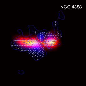
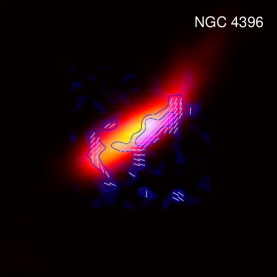
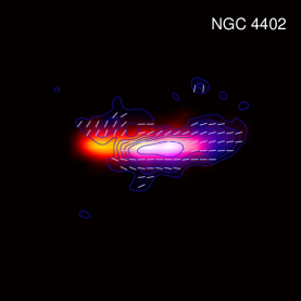
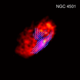
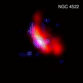
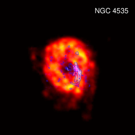
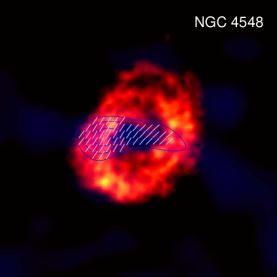
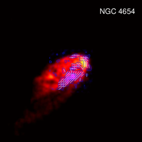
Figure 1: Polarized radio ridges in comparison with the H i emission. Six-centimetre polarized intensity contours and blue colour[2004AJ....127.3375V, 2007A&A...464L..37V, 2007A&A...471...93W, 2010A&A...512A..36V] overlaid on H i intensity data[2009AJ....138.1741C] (red-to-yellow). The short lines represent the polarization vectors rotated by 90 degrees, hence delineating the orientation of the magnetic field in the draping layer uncorrected for Faraday rotation (hereafter referred to as ‘B-vectors’). The contour levels are $(4,8,12,16,20,30,40,50)\times\xi\mu$Jy ($\xi=5$ for NGC 4522; $\xi=8$ for NGC 4388, NGC 4396, NGC 4402, NGC 4654; $\xi=10$ for NGC 4535; $\xi=11$ for NGC 4501) and $(4,5,6)\times 90\mu$Jy for NGC 4548. We employed an additive colour scheme: if the polarized intensity were perfectly correlated with the H i, the two colours should add up to ‘white’ at the region of maximum emission. The fact that they do not in most cases is one reason for an extragalactic origin of the radio emission (see text for more detail).

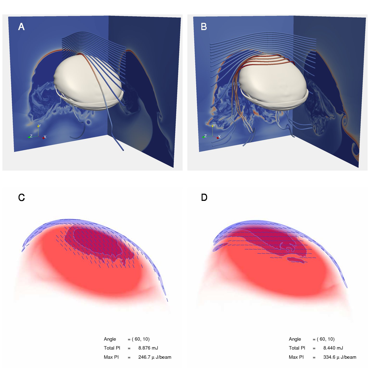
Figure 2: Simulations of spiral galaxies interacting with a uniform cluster magnetic field. (Top) The grey isosurface represents an upwards moving galaxy in an Athena simulation[StoneEtAl2008, 2005JCoPh.205..509G, 2008JCoPh.227.4123G]. Representative magnetic field lines and cut planes through the stagnation line of the flow are coloured by the magnitude of the local magnetic field strength. (Bottom) Projected density (red) and a simulated $6\,\mathrm{cm}$ synchrotron emission map, with polarized intensity shown in blue contours (using the same contour levels and beam sizes of $18^{\prime\prime}\times 18^{\prime\prime}$ as recent observational work[2008A&A...483...89V]; for details, see Supplementary Information). Lines indicate local polarization direction rotated by ninety degrees (‘B-vectors’), to indicate the local magnetic field orientation. The left and right panels differ only in the initial magnetic field orientation; this difference clearly shows up in the simulated radio observations.

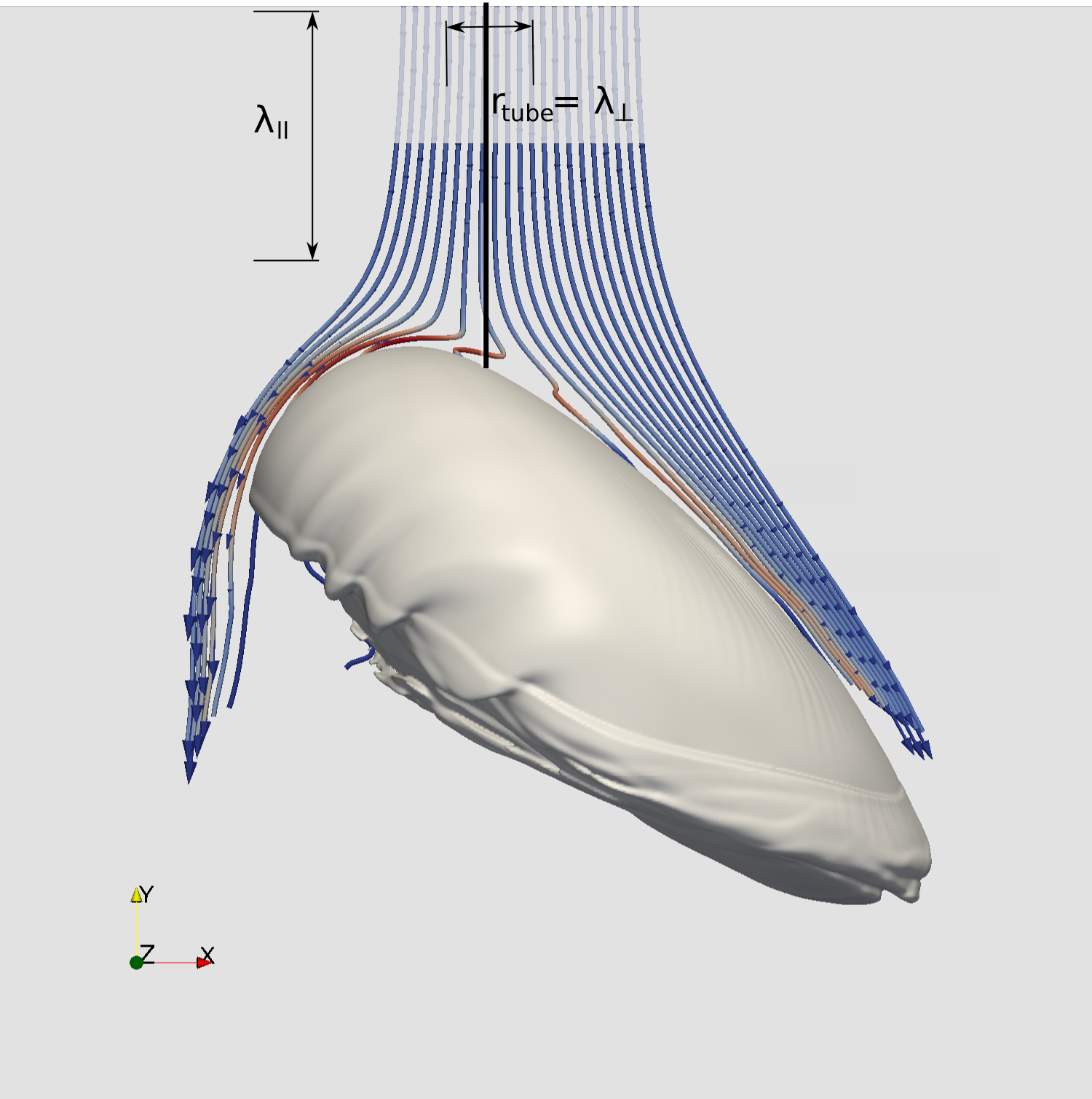
Figure 3: Streamlines in the rest frame of the galaxy. The arrows indicate the magnitude of the flow and the colours the magnetic energy density that they encounter. As the uniform flow approaches the galaxy it decelerates and gets deflected. Only those streamlines initially in a narrow tube of radius $\lambda_{\perp}$ from the stagnation line become part of the draping layer. The streamlines that do not intersect the tube get deflected away from the galaxy, become never part of the drape and eventually get accelerated as they have less volume to transport the plasma past the galaxy (known as the Bernoulli effect). As we will see in Fig. 4, magnetic field must be coherent along the direction of motion on a scale greater than $2\,\lambda_{\parallel}$ for a significant draping signal to be seen. We note that the streamlines are almost identical for our simulations with different realizations of the magnetic field. Note a visible kink feature in some draping-layer stream lines as the solution changes from the hydrodynamic potential flow solution to the draped layer, where the back reaction plays a significant role.

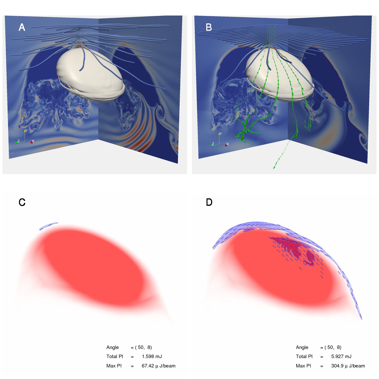
Figure 4: Simulations of spiral galaxies interacting with a non-uniform cluster magnetic field. As in Fig. 2, but with cluster magnetic fields in a force-free helical configuration with a given coherence length in the direction of motion of the galaxy. (Left) Wavelength of the helix is $14\,\mathrm{kpc}$, less than the radius of the galaxy. (Right) Wavelength is $57\,\mathrm{kpc}$, larger than the diameter of the galaxy. In (B), we also show representative streamlines in green, with arrow size indicating speed. The flow speed is greatly reduced in the draping boundary layer. The radio emission is greatly reduced for (C) because of depolarization by the superposition of different field orientations in the draping layer. In (D), note the increased complexity of the B-vectors compared to Fig. 2D which is due to the helical structure of the ambient field.

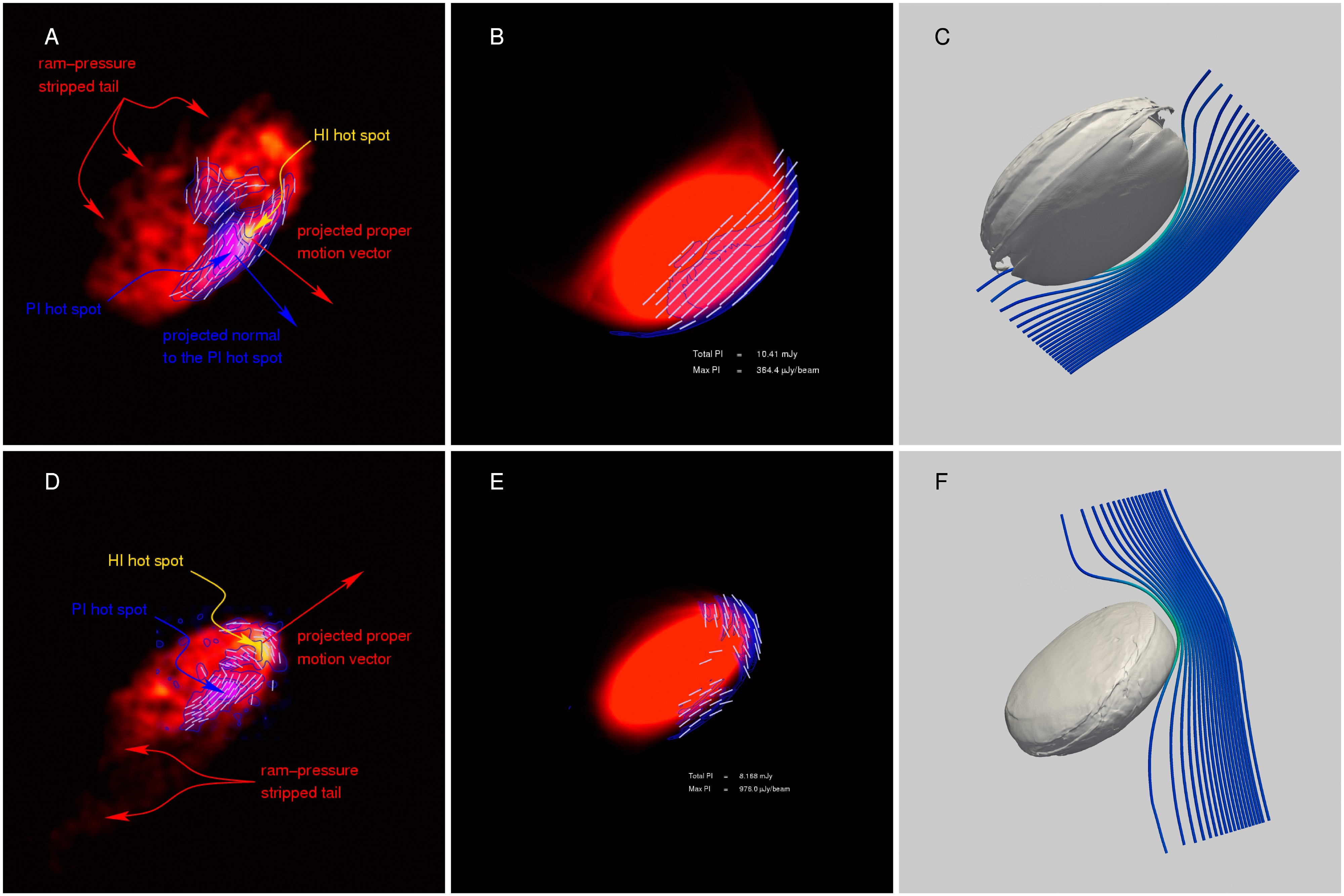
Figure 5: Polarized radio emission: observations versus simulation. (Left) H i emission[2009AJ....138.1741C] of two spirals (A: NGC 4501, and D: NGC 4654) tracing the neutral hydrogen distribution that is severely affected by the ram pressure resulting from the galaxies’ motion in the intra-cluster plasma (red-to-yellow). Over-plotted are the polarized intensity (PI) of the radio synchrotron ridges[2007A&A...464L..37V] at $6\,\mathrm{cm}$ (blue and contours) with the B-vectors indicated in white. (Middle) Simulated synchrotron maps that are selected from the uniform field models. (Right) Shown is a 3D volume rendering of our best matching galaxy model (shown with grey isosurfaces) and representative magnetic field lines (see Supplement for details). The misalignment of the H i and PI hot spots for NGC 4654 might point to a geometric bias (upstream magnetic field has a non-negligible line-of-sight component) as our numerical model suggests; hence we omitted plotting the projected normal to the PI hot spot for this galaxy.

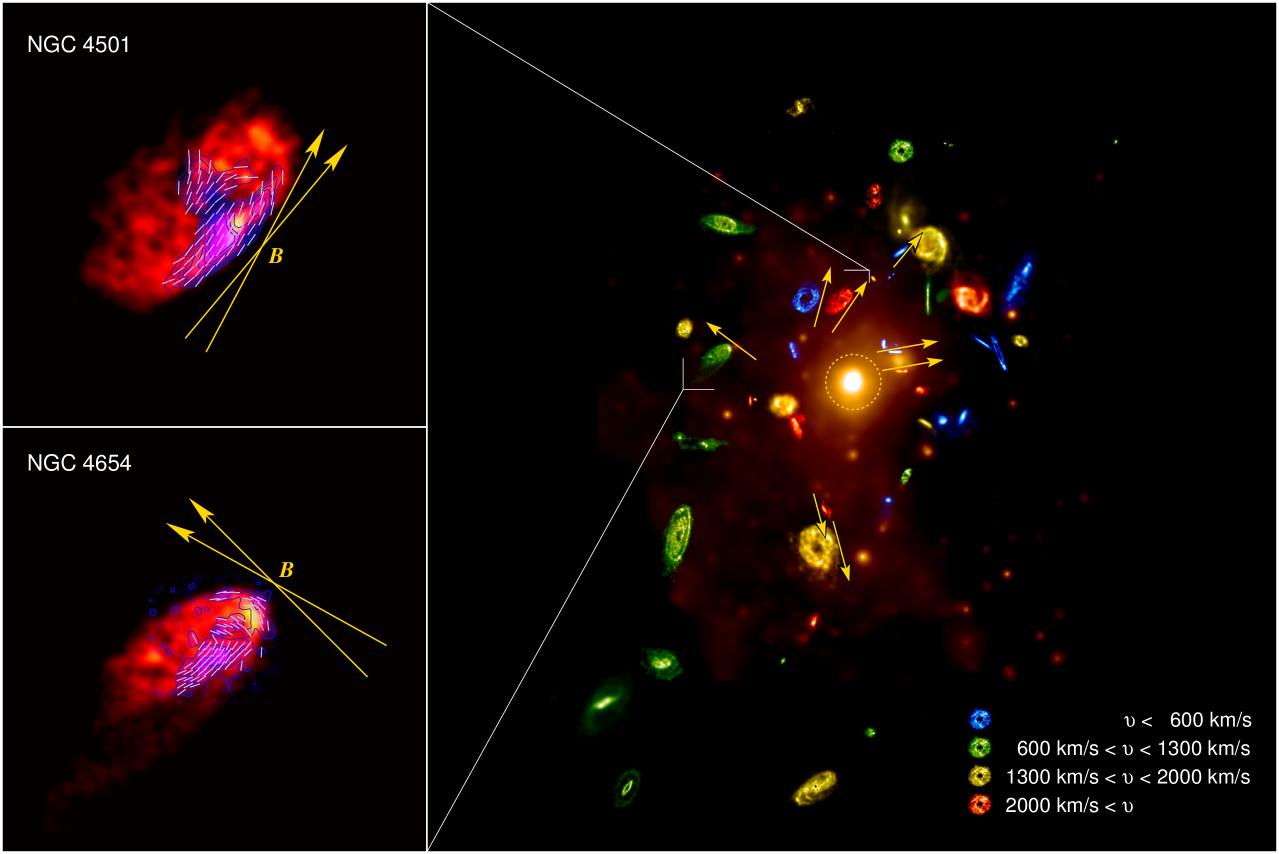
Figure 6: Mapping out the magnetic field orientations in the Virgo galaxy cluster as inferred from the polarized synchrotron emission ridges of cluster spirals. (Left) H i intensity data[2009AJ....138.1741C] (red-to-yellow) overplotted with $6\,\mathrm{cm}$ polarized intensity contours and B-vectors[2007A&A...464L..37V] (blue). The direction of the B-vectors directly measures the projected local orientation of the cluster magnetic fields B (yellow) with the range of plausible field orientations indicated by the double-arrow. (Right) ROSAT X-ray image of the Virgo cluster[1994Natur.368..828B] (orange colour scale). Over-plotted is the H i emission of Virgo spirals in the VIVA survey[2009AJ....138.1741C] that is colour coded according to their velocities, and the green colour scale coincides with the cluster’s mean heliocentric velocity of 1100 km sec^-1 (after image by Chung et al.[2009AJ....138.1741C]). Galaxies are magnified by a factor of 10. The yellow arrows indicate the projected orientation of the magnetic field in Virgo at the position of the galaxies that have high-resolution polarized radio data. Note that the arrowheads could also point in the opposite direction because of the $n\pi$-ambiguity of inferring magnetic orientations from synchrotron polarization. We find that the magnetic field is preferentially oriented radially which is very suggestive that the magneto-thermal instability is operating[2000ApJ...534..420B, 2008ApJ...688..905P] as it encounters the necessary conditions outside a spherical region with radius 200 kpc[1994Natur.368..828B] (indicated with the yellow dotted circle).

14

 
Supplementary Information for the Nature Physics Article
“Detecting the orientation of magnetic fields in galaxy clusters”

Christoph Pfrommer¹, L. Jonathan Dursi^2,1

1 Simulations

1.1 Modelling the galaxy

In our model, we deliberately choose to neglect interstellar magnetic fields, the galaxies’ rotation, winds and outflows, or even the multiphase structure of the galaxies for the following reasons: we wanted to study a clean controlled experiment without complications such as numerical reconnection and the mentioned properties do not have any immediate influence on the physics of draping. Moreover, since there is no evidence in the data of these galaxies for any outflows, we are save to neglect them. All edge-on galaxies in our sample show extraplanar polarised emission which is impossible to reconcile in a model where the polarised emission is due to interstellar magnetic fields or intracluster magnetic fields that interact with the neutral component of the interstellar medium. Similarly, the coherence of the observed polarised emission across entire galaxies requires a coherent process that works on galactic scales: the strong turbulent magnetic field on small scales found in the star forming regions is incapable of explaining this fact. Shearing motions seeded by galactic rotation do not come into questions as they fail to explain the extraplanar polarised emission as well as the fact that the polarised synchrotron emission leads the HI distribution in some cases. Hence we are forced to consider coherence of the intracluster magnetic field on scales at least as large as these galaxies under consideration. We will discuss this in more detail in Sect. 6.

The magnetohydrodynamical (MHD) simulations described in this work were performed using the Athena code[GardinerStone2005, GardinerStone2008, StoneEtAl2008], a freely-available uniform-grid dimensionally unsplit MHD solver for compressible astrophysical flows. Our earlier work[2008ApJ...677..993D] used the Flash code[flashcode, flashvalidation] which had the great advantage of having an adaptive mesh; however for these simulations with roughly sonic flow, dimensionally split solvers are susceptible to the well-known stationary shock instability and thus Flash was unsuitable.

Our simulations were of an ideal, perfectly conducting, adiabatic, $\gamma=5/3$ fluid. The simulations were in the frame of the galaxy, with an incoming wind with velocity $1000\,\mathrm{km}\,\mathrm{s}^{-1}$ of ambient fluid with $P=1.67\times 10^{-12}\,\mathrm{dyne}\,\mathrm{cm}^{-2}$ and $\rho=m_{\mathrm{p}}\,10^{-4}\,\mathrm{cm}^{-3}$ which results in a number density $n=\rho/(\mu\,m_{\mathrm{p}})=1.7\times 10^{-4}\,\mathrm{cm}^{-3}$ assuming primordial element composition with a mean molecular weight of $\mu=0.6$. Because the magnetic draping is solely an effect occurring at the wind/galaxy contact discontinuity, and does not depend on the internal structure of the galaxy at all, the spiral galaxy was simply modelled as a cold dense oblate ellipsoid of gas with an axis ratio $q=0.1$ initially centred at $(0,0,0)$ with no self-gravity. It was in pressure equilibrium with the ambient cluster medium , had a gently-peaked density profile which smoothly matches on to the ambient medium, $\rho(r_{e})=\rho_{0}(\cos(\pi r_{e}/r_{e,0})+1)/2$ where $r_{e}$ is the elliptical radius, $r_{e,0}$ is the elliptical radius of the galaxy, and $\rho_{0}$ is the central density of the ‘galaxy’.

A schematic of the geometry modelled is shown in Figure 1. The direction of motion for the galaxy was taken to be along positive $y$ direction, so that the wind seen by the galaxy moves in the negative $y$ direction. For the simulations considered here, the normal of the galaxy’s disk was inclined at a $45^{o}$ angle to the direction of motion. The disk of the galaxy was taken to have a radius of $20\,\mathrm{kpc}$. The simulation domain was generally taken to be $[-28.3\,\mathrm{kpc},28.3\,\mathrm{kpc}]$$\times$ $[-39.6\,\mathrm{kpc},28.3,\mathrm{kpc}]$$\times$ $[-28.3\,\mathrm{kpc},28.3\,\mathrm{kpc}]$. Because the draping occurs super-alfvénincally at the contact discontinuity, varying domain sizes or boundary conditions in early simulations were not seen to affect the structure of the boundary layer at all. The turbulent wake, very interesting in its own right, did show some modest reaction to domain size and boundary conditions, but is not the focus of this work. The boundary conditions used here were fixed inflow at velocity $\upsilon_{w}$ at the top ($+y$) boundary, and zero-gradient ‘outflow’ at the bottom ($-y$) and horizontal ($\pm x,z$) boundaries.

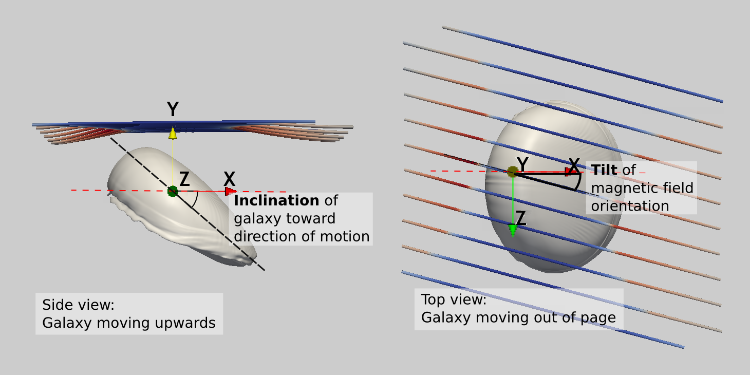
Supplementary Figure 1: Schematic of simulation geometry. Shown is the orientation of the model galaxy (grey isosurface) and the magnetic fields, with respect to the simulation coordinate system. The galaxy moves in the $y$ direction, with an inclination along the $z$-axis, and the field is generally taken to be uniform with some ‘tilt’ angle along the $y$-axis from the $x$-axis.

In initial experiments with the top boundary, rather than start the inflow at near-sonic we allowed the flow to ‘ramp up’ over some characteristic time. This had the important effect of reducing large transients in small initial high Mach number simulations, but had no effect for these runs, and was not used here. The boundary condition is also responsible for the magnetisation of the ambient medium; at time zero, there is no magnetic field anywhere in the domain; the magnetic field is advected in with the inflow from the $+y$ boundary.

1.2 Magnetic field strength and resolution study

The simulations here are scale-free and can be described solely in terms of dimensionless quantities. For modelling galaxies orbiting within a galaxy cluster, our length scale (the size of a typical spiral galaxy) is more or less a given. The velocity scale is set to be roughly sonic (we choose here $\upsilon\approx 1000\,\mathrm{km}\,\mathrm{s}^{-1}$), as the same gravitational potential sets both orbit speeds and the gas thermodynamic profiles. Our choice implies somewhat subsonic motions, ${\cal{M}}=\upsilon_{\mathrm{gal}}/c_{\mathrm{s}}=\upsilon_{\mathrm{gal}}/\sqrt{\gamma P/\rho}=\sqrt{3/5}\approx 0.77$.

With length and velocity scales given, the timescale is then set, as well. Remaining is only the magnetic field parameter describing the ambient magnetic field strength in the cluster. This can be given by the ‘plasma beta’, the ratio of ambient gas pressure to magnitude of the ambient magnetic field, $\beta=P/\sqrt{B^{2}/(8\pi)}$, or alternatively the Alfvénic Mach number, ${\cal{M}}_{A}=\upsilon_{\mathrm{gal}}/\upsilon_{A}={\mathcal{M}}\,\sqrt{\beta\gamma/2}$.

The plasma beta in the outskirts of a galaxy cluster such as Virgo is uncertain, but is expected to be in the range $300\ {\raise-1.93748pt\hbox{$\buildrel<\over{\sim}$}}\ \beta\ {\raise-1.93748pt\hbox{$\buildrel<\over{\sim}$}}\ 10^{5}$. This can be seen by taking a central magnetic field $B_{0}\simeq 8\,\mu$G of similar strength as it is inferred in other clusters[2002ARA&A..40..319C, 2002RvMP...74..775W, 2004IJMPD..13.1549G, 2005A&A...434...67V, 2009arXiv0912.3930K] and using a density of $n\simeq 10^{-4}\,\mathrm{cm}^{-3}$ which is approximately a factor of $\delta=n_{0}/n\simeq 10^{3}$ lower compared to the central value $n_{0}$[2002A&A...386...77M]. We estimate its value at a cluster radius of $\sim 600$ kpc (where we observe these galaxies) to $B\simeq B_{0}\,\delta^{-\alpha_{B}}\simeq(0.02,\ldots,0.25)\,\mu$G, with $\alpha_{B}=(0.5,\ldots,0.9)$ (see Fig. 15). The choice $\alpha_{B}=0.7$ corresponds to the flux freezing condition. We employ a plausible range for $\alpha_{B}$ as determined from cosmological cluster simulations[1999A&A...348..351D, 2001A&A...378..777D] and Faraday rotation measurements[2005A&A...434...67V]. We note, however, that these techniques are not capable of resolving or measuring small-scale turbulent dynamo processes in the cluster outskirts and potentially miss the field amplification by these processes (as long as the resulting field strength is small compared to that in the cluster centre). Hence the true plasma beta in the outskirts of galaxy clusters could be in the range $10^{2}\ {\raise-1.93748pt\hbox{$\buildrel<\over{\sim}$}}\ \beta\ {\raise-1.93748pt\hbox{$\buildrel<\over{\sim}$}}\ 10^{3}$ as suggested by recent theoretical work[2006PhPl...13e6501S].

Resolution constraints, however, mean that we aren’t completely free to choose arbitrary $\beta$. In the draping region, along the stagnation line, we expect from earlier analytic kinematic work[1980Ge&Ae..19..671B, lyutikovdraping, 2008ApJ...677..993D]

$$B\simeq B_{0}\left[1-\left(\frac{R}{R+s}\right)^{3}\right]^{-1/2},$$ (1)

where $s$ is the distance along the stagnation line from the leading edge of the (assumed spherical) projectile; for $s/R\ll 1$,

$$B(s)\simeq B_{0}\sqrt{\frac{R}{3s}}.$$ (2)

In reality, the field growth is truncated where the back reaction becomes significant, $\alpha\rho_{\mathrm{icm}}\upsilon_{\mathrm{gal}}^{2}\approx B^{2}/(8\pi)$, and so the drape thickness should be

$$l_{\mathrm{drape}}\simeq\frac{1}{6\alpha{\cal{M}}_{A}^{2}}\,R\simeq\frac{1}{3\alpha\beta\gamma{\cal M}^{2}}\,R$$ (3)

where ${\cal M}\approx 1$ for our case, and in our previous work with spherical projectiles, $\alpha\approx 2$. Imposing the constraint $l_{\mathrm{drape}}\ {\raise-1.93748pt\hbox{$\buildrel>\over{\sim}$}}\ \Delta x$ for an object of size $R=L\,\sqrt{2}/4$ where $L$ is the size of our box, we derive a resolution-based restriction on $\beta_{\mathrm{sim}}$:

$$\beta_{\mathrm{sim}}\ {\raise-1.93748pt\hbox{$\buildrel<\over{\sim}$}}\ \frac{\sqrt{2}}{12\alpha\gamma{\cal M}^{2}}N$$ (4)

where $N$ is the number of points in the domain. Computational requirements lead us to resolution of $(N_{x},N_{y},N_{z})=(640,768,640)$, meaning that the natural $\beta_{\mathrm{sim}}$ to choose is $\beta_{\mathrm{sim}}\approx 40$; smaller plasma beta parameters lead to a thicker layer. As a compromise between the resolution requirements and fidelity to the physical conditions of the intra-cluster medium (ICM), we choose $\beta_{\mathrm{sim}}=100$.

From the discussion above, then, using the parameter $\alpha\approx 2$ from our simulations of spherical projectiles, we would expect $l_{\mathrm{drape}}\approx R/600=33\,\mathrm{pc}$, or $\Delta x\approx 2.7l_{\mathrm{drape}}$. However, $\alpha$ is a geometric parameter; the thickness of the layer is set by the requirement that at the top of the layer, flow and excess magnetic pressure do enough work on the tension of the magnetic field lines to push them around the obstacle. Thus, $\alpha$ depends sensitively on the geometry of both the flow and the magnetic field. In our highly flattened geometry representing a galaxy, the layer thickness is greater than over a sphere for zero inclination. We note that the layer becomes thinner for increasing inclinations of the galaxy with respect to the direction of motion[D&P] which increases the requirements for the numerical resolution that is need to resolve the layer.

Supplementary Figure 2: Resolution study. Plotted is the magnetic energy density (in $10^{-12}\,\mathrm{erg}\,\mathrm{cm}^{-3}$) along the stagnation line for one of our fiducial models (shown in the left hand side of Fig. 2 of the main body), as points connected by a solid line, and the results for the same elapsed simulation time for a simulation with twice the number of resolution elements in each direction – $(N_{x},N_{y},N_{z})=(1280,1536,1280)$ shown with a dashed line and points. The high resolution simulation contained 2.5 billion points, required 300,000 CPU hours, and generated 1.2 TB of data. We see that the peak of the magnetic energy density - the draping layer - seems to be of order 100-150pc thick, and is resolved by two grid cells even in the lower resolution simulation. The main difference between the two is a somewhat reduced magnetic field strength in the lower-resolution case, possibly due to the increased numerical magnetic diffusion at the lower end of the layer.

The calculation of $\alpha$ for varying geometries is beyond the scope of this work, but for our geometry, we can measure the thickness of the drape layer in our simulations, and run resolution tests to ensure we correctly resolve the layer. This is done in Fig. 2, where we compare our fiducial simulations with an inclination of 45 degrees (solid line) to a simulation of double the resolution. A rendering of the high-resolution simulation is shown in Fig. 3. We see that even in our fiducial resolution case we resolve the layer thickness by two cells, although the field is somewhat reduced from its true value due to increased numerical diffusion. We also note that the stagnation line is the point of maximum field line compression and places the most stringent condition on resolution. Well off the stagnation line, the magnetic drape is clearly well resolved by four or more grid cells. However, it is the stagnation line, where the magnetic field is greatest and in the thinnest layer, which is most relevant for the synchrotron signal from the draped layer.

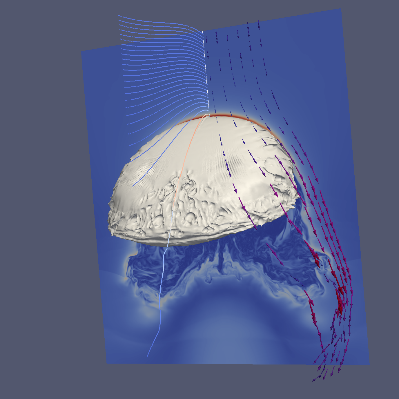
Supplementary Figure 3: Rendering of the high resolution run. Plotted are field lines along the stagnation line, and velocity vectors coloured and sized by magnitude of velocity. This is the high resolution case that is used for comparison; just the rendering of this data required 256 processors on SciNet’s GPC cluster.

1.3 Magnetic field orientations

The orientation of our galaxy model with respect to the direction of motion and the ambient magnetic field are parameters we are rather free to choose.

For the ’inclination’ of the galaxy (the angle between the normal to the galactic plane and the velocity of the galaxy), a face-on orientation (inclination of zero) is somewhat trivial due to the high degree of symmetry and closely follows our previous work[2008ApJ...677..993D], so is unnecessary to reproduce here. At the other extreme, an edge-on orientation (inclination of 90 degrees) is somewhat less symmetric, but has a small phase-space for occurrence, and is too sensitive to the differences between our galaxy model and a realistic galaxy. Thus the simulations performed for this work typically had intermediate inclinations. The simulations in Figs. 1 and 2 had an inclination of 45 degrees as a representative orientation, breaking enough symmetries to give non-obvious results.

The ’tilt’ between the magnetic field orientation and the plane defined by the galaxy velocity vector and its normal is taken to be constant in our models of a uniform magnetic field, from zero to ninety degrees. In Sects. 2.4 and 5.2 we discuss some intermediate cases in the context of determining how accurately one can infer magnetic field orientation. We also consider some cases of a time-varying orientation of magnetic field.

In addition to a homogeneous magnetic field in our initial conditions, we want to explore a field with a characteristic scale in order to address the question on how to measure the magnetic correlation length with our proposed effect. Analytic force-free magnetic field configurations with an isotropic 3D-correlation scale do not exist. There is a number of non-isotropic 3D force free solutions. Since we are most interested in variations along the direction of motion as we want to study how these imprint themselves as changes in the expected polarisation signal. Hence, we decided to maintain the homogeneous field in the plane perpendicular to the direction of motion, but to allow for variations of it along the direction of motion (that we take to be the $y$-axis). Employing the force-free conditions, namely

$$\mathbf{\nabla}\cdot\textbf{{B}} = \textbf{{0}},$$ (5)

$$(\mathbf{\nabla}\times\textbf{{B}})\times\textbf{{B}} = \textbf{{0}},$$ (6)

we arrive at one solution $\textbf{{B}}=B_{0}(\cos(ky),0,\sin(ky))^{T}$ that satisfies these equations. It represents a uniform field with an orientation that rotates along the $y$-direction (our assumed direction of motion) thereby forms a helical structure.

2 Physics of magnetic draping

Here, we are summarising the most important results regarding the physics of magnetic draping over moving objects while we refer the reader to previous work[2008ApJ...677..993D] for a more detailed study.

2.1 Magnetic energy of the draping layer

We just saw that the magnetic energy density in the draping layer, $\varepsilon_{B}\simeq\alpha\rho\upsilon^{2}$, is solely given by the ram pressure wind and completely independent of the strength of the ambient cluster fields. However, the total energy in the draping sheath is proportional to the energy density of the ambient cluster field. We demonstrate this analytically for the simple example of a sphere with radius $R$ and volume $V_{\mathrm{sph}}$, while we assume a constant thickness of the drape $l_{\mathrm{drape}}$ (see Eqn. 3). The total energy in the drape covering the half sphere with an area $A=2\pi\,R^{2}$ is given by

$$E_{B,\,\mathrm{drape}} = \frac{B_{\mathrm{drape}}^{2}}{8\pi}\,A\,l_{\mathrm{drape}}=\frac{B_{\mathrm{drape}}^{2}}{8\pi}\,\frac{A\,R}{6\alpha\,{\mathcal{M}}_{A}^{2}}$$ (7)

$$= \alpha\rho\upsilon_{\mathrm{gal}}^{2}\,\frac{A\,R}{6\alpha}\,\frac{B_{\mathrm{icm}}^{2}}{4\pi\,\rho\upsilon_{\mathrm{gal}}^{2}}=\frac{1}{2}\,\varepsilon_{B,\,\mathrm{icm}}\,V_{\mathrm{sph}}.$$

In our case of draping over a galaxy, we expect geometrical factors to enter so that our assumptions will be modified and we need to numerically simulate and study this problem in more detail[D&P].

2.2 Developing the draping layer

As suggested by Eqn. 7, the time necessary to sweep up the magnetic drape is much shorter than the orbital crossing time (the time it takes for a galaxy to cross the entire cluster; $\tau_{\mathrm{cross}}=2\,R_{\mathrm{cluster}}/\upsilon_{\mathrm{gal}}$) of the galaxies in the cluster. We have $E_{B,\,\mathrm{drape}}\simeq 0.5\,\varepsilon_{B,\,\mathrm{icm}}V_{\mathrm{gal}}\simeq 0.5\,E_{B,\,\mathrm{icm}}(<V_{\mathrm{gal}})$. Energy conservation tells us that we need at least half a galactic crossing time (the time it takes for a galaxy to travel its own size; $\tau_{\mathrm{c}}=2\,R_{\mathrm{gal}}/\upsilon_{\mathrm{gal}}$) to get the magnetic energy in the drape - and possibly a factor of a few more as not all the magnetic energy represented by field lines in the sweep-up region ahead of the galaxy ends up in the drape as the circulation flow around the galaxy establishes itself and magnetic back reaction starts to build up causing longer residency timescales of the field lines in the drape. Once the magnetised boundary layer around the galaxy is set up, the galaxy is very ‘sticky’; field lines that enter the boundary layer stay there for on order ten galactic crossing times.

Supplementary Figure 4: Time evolution of field strength. Shown here is the contribution to magnetic energy from the $x$ component of the magnetic field integrated through the domain for one of our fiducial simulations with the ambient magnetic field oriented in the $x$ direction. It is seen to level off by $t\approx 82.8\,\mathrm{Myr}$; most of our analysis in this work is based on snapshots of the simulation at time $t=85.25\,\mathrm{Myr}$. Simulations were run to $t=103.5\,\mathrm{Myr}$; when there are differences these are noted.

Exactly how long the boundary layer takes to become established, however, is a subtle question, and one we don’t address here. We note instead that empirically here and in previous work[2008ApJ...677..993D] we find that within five or so galactic crossing times the layer seems to have established a steady state. Plotted in Fig. 4 is the $x$-contribution to the magnetic energy in the simulation domain in a fiducial simulation where the field was oriented in the $x$ direction. A steady state begins to be reached by about $t=82.8\,\mathrm{Myr}$; our simulations run to $103.5\,\mathrm{Myr}$, and most of our analysis is done on snapshots from $t=85.25\,\mathrm{Myr}$.

It is important to note that the buildup of the magnetic draping layer is a boundary-layer effect, and not due to compression. The flows considered here are roughly sonic, and any resulting adiabatic compressions of fluid elements (and of the field frozen into them) is much too small to result in such a large magnetic field enhancement. Indeed, as Fig. 5 shows, the peak of magnetic field energy actually corresponds to a local drop of density. The data from this plot was taken from the high-resolution simulation shown in Fig 3.

Supplementary Figure 5: Density and magnetic field along the stagnation line. The density (in units of ambient density) along the stagnation line of a very high-resolution draping run plotted with a solid line and using the logarithmic scale on the left, overplotted with the magnetic energy density (in units of the ambient magnetic energy density) plotted with a dashed line and using the linear scale on the right. Data was taken from a snapshot in the simulation when the magnetic drape is still being established. Note that the peak of the magnetic energy density occurs where there is actually a small drop in local density, because of the influence of the now dynamically-important magnetic pressure. Crucially, the magnetic field pileup is not a compression effect.

2.3 Dissecting the draping process – draping of turbulent fields

Here we will argue that our choice of homogeneous fields in the plane perpendicular to the direction of motion is in fact representative and captures the essence of the observable draping signal in the polarised synchrotron emission even if we were to consider turbulent fields. To this end, we need to understand which region in the upstream ends up the the magnetic draping boundary layer. In other words, we want to know which scale perpendicular to the direction of motion is mapped into the drape. In our previous work, we demonstrated that outside the draping sheath in the upper hemisphere along the direction of motion, the smooth flow pattern resembles that of an almost perfect potential flow solution[2008ApJ...677..993D]. The thickness of the magnetic boundary layer $l_{\mathrm{drape}}$ is given by Eqn. 3. Hence, we want to derive the impact parameter of the streamline to the stagnation line, that is tangent to the outermost boundary layer. Fluid further away from the stagnation line than this critical impact parameter is deflected away from the galaxy and will never become part of the draping layer. Using for simplicity the spherical approximation, we previously derived in Appendix A.2 an approximate equation for the impact parameter $p$ in the region close to the sphere[2008ApJ...677..993D],

$$p=\sqrt{3sR}\,\sin\theta.$$ (8)

Here $s=r-R$ is a radial variable measured from the contact of the sphere with radius $R$, and $\theta$ denotes the the usual azimuthal angle measured from the stagnation line. Taking $s=l_{\mathrm{drape}}$, we derive a critical impact parameter

$$p_{\mathrm{cr}}=\frac{1}{\sqrt{\alpha\beta\gamma}}\frac{R\,\sin\theta}{{\mathcal{M}}}\simeq\frac{R\,\sin\theta}{\sqrt{2\beta}}\simeq\frac{R}{15}.$$ (9)

In our previous work with spherical projectiles[2008ApJ...677..993D], $\alpha\approx 2$ and we adopted numerical values used in our simulation, i.e. ${\cal M}=1/\sqrt{\gamma}$ and $\beta=100$. In the last step we adopted the condition that the streamline never intercepts the draping region, i.e. $\theta=\pi/2$. We note that most of the polarised intensity comes from a region $\theta<\pi/6$ which implies a critical impact parameter of $R/30$ for streamlines to intercept the synchrotron emitting region. The theoretically expected value of Eqn. 9, $p_{\mathrm{cr}}\simeq R/15$, agrees well with that found in our simulations (Fig. 3), where $p_{\mathrm{cr}}\simeq R/10\simeq 2$ kpc. The differences can easily be accounted by the differing geometry that might modify the effective curvature radius in the vicinity of the stagnation line (and possibly cause a different value of $\alpha$) and/or magnetic back-reaction in the draping sheath that could also offset the streamlines with respect to the simplified case of a potential flow.

These considerations suggest a criterion that the magnetic coherence scale has to meet for magnetic fields to be able to drape and modify the dynamics of the draped object. This draping criterion reads

$$\frac{\lambda_{B}}{2\,R}\ {\raise-1.93748pt\hbox{$\buildrel>\over{\sim}$}}\ \frac{1}{\sqrt{\alpha\beta\gamma\,{\mathcal{M}}^{2}}}.$$ (10)

Here $R$ denotes the curvature radius of the working surface at the stagnation line (which can be identified as its initial simulation value while it might be modified for cases of marginal stability due to hydrodynamic instabilities), $\alpha\approx 2$ (as measured for spherical objects in our earlier work[2008ApJ...677..993D] and can also be slightly modified of order unity for non-spherical cases), $\gamma=5/3$, and ${\mathcal{M}}$ is the sonic Mach number. We can test our formula with magnetohydrodynamical simulations of fossil AGN bubbles that rise buoyantly in a cluster atmosphere with tangled magnetic fields of various coherence scale[2007MNRAS.378..662R]. These simulations have a plasma beta parameter of $\beta=20$ and the bubbles have a sonic Mach number of ${\mathcal{M}}\simeq 0.25$[Ruszkowski2010]. The condition for bubble stability due to draped magnetic fields reads

$$\frac{\lambda_{B}}{R}\ {\raise-1.93748pt\hbox{$\buildrel>\over{\sim}$}}\ \frac{2}{\sqrt{2\times 20\times\frac{5}{3}\times 0.25^{2}}}\simeq 1.$$ (11)

These simulations explored two archetypal cases. (1) The ‘draping case’ had a magnetic coherence scale was much larger than the bubble radius, $\lambda_{B}/R\simeq 4.8$. It showed that draping occurs under these circumstances (just as our formula of Eqn. 10 suggested) and showed the ability of the draped magnetic fields to suppress Kelvin-Helmholtz instabilities. (2) The ‘random case’ had a magnetic coherence scale that was of order the initial bubble radius, $\lambda_{B}/R\simeq 0.96$ – hence it was at marginal stability according to Eqn. 10. In such a case, hydrodynamical instabilities start to flatten the contact surface which increases the curvature radius at the stagnation line; an effect that violates the condition for draping of Eqn. 10. Hence, in the absence of draping the interface cannot be longer stabilised against the shear so that a smoke ring develops as these simulations show! We caution the reader that the quantitative predictions stated here need to be thoroughly tested in future simulations that will help to consolidate the picture put forward.

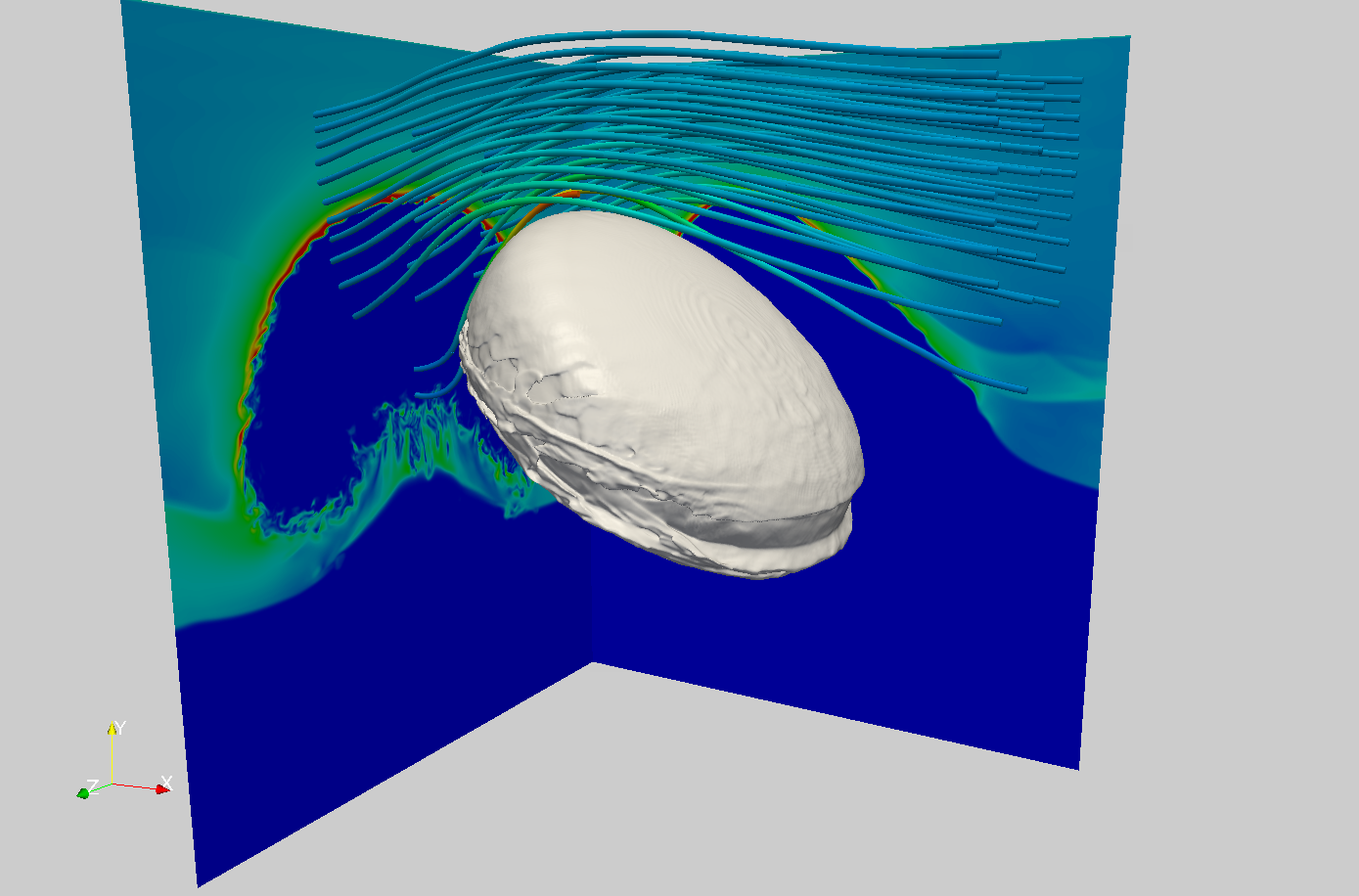
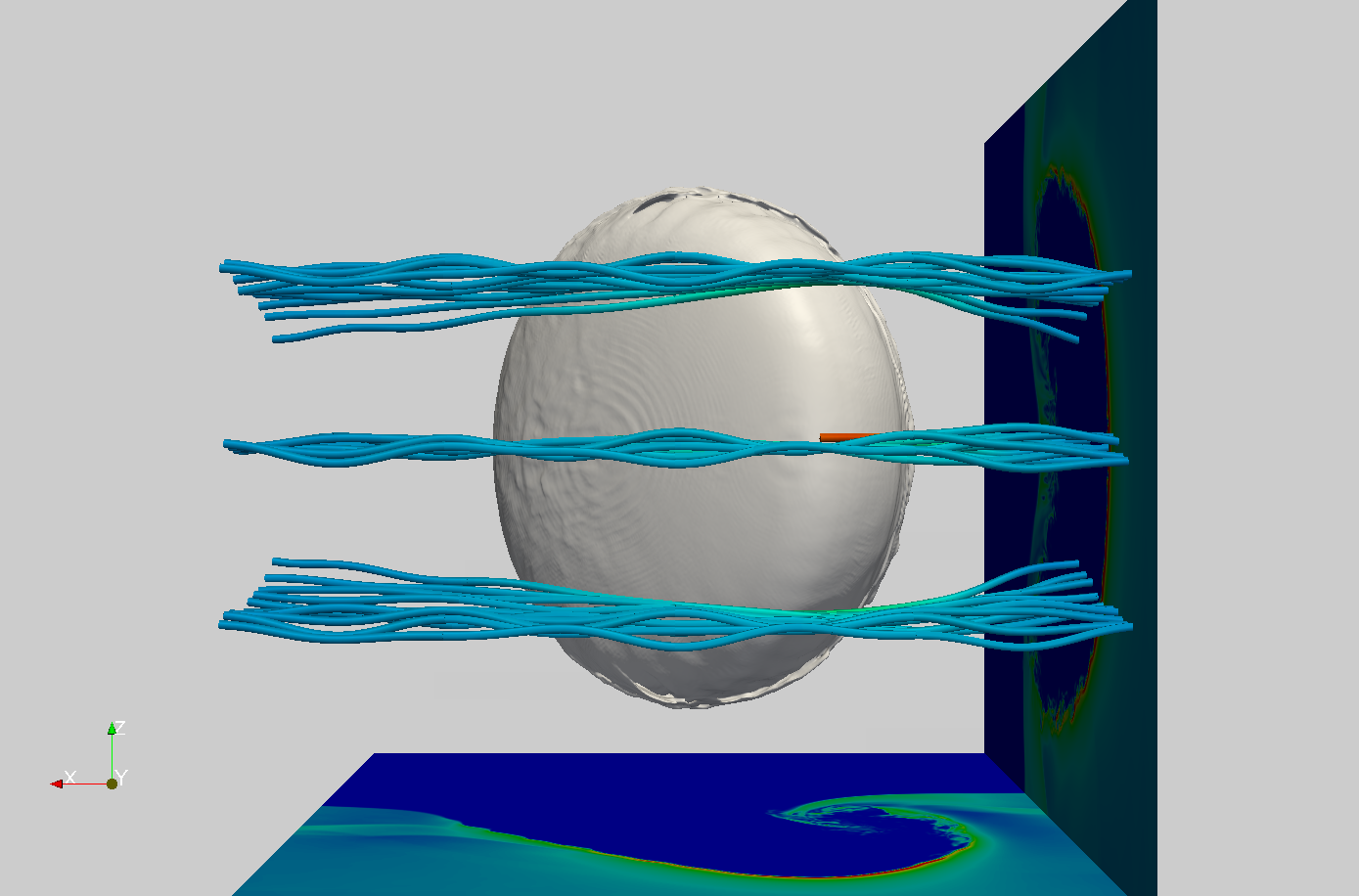
Supplementary Figure 6: Simulating magnetic draping of perturbed homogeneous fields: Shown are views from the side and top of a simulation with homogeneous guide fields (similar to those in Fig. 2A). However, we added a sinusoidal perturbation that was pointing perpendicular to the guide field and direction of motion that we also varied along the direction of motion. The energy density in the perturbation was 1/10 of that in the guide field. Note that we still form a dynamically important draping sheath.

In Figure 4 we demonstrated that the magnetic coherence length parallel to the direction of motion needs to be at least of order the galaxy’s size for polarised emission to be significant. Otherwise, the rapid change in field orientation leads to depolarisation of the emission. For the sake of the following argument, we assume that the ICM were turbulent and statistically isotropic. Assuming a Kolmogorov spectrum with a coherence scale that is larger than the galaxy’s diameter, the ratio of magnetic energy density of that large scale to the small scale that is mapped onto the polarised emission signal is given by

$$\frac{\delta B)^{2}}{(\delta B_{0})^{2}}=\left(\frac{k}{k_{0}}\right)^{-2/3}\simeq 30^{2/3}\simeq 10.$$ (12)

We simulated such a case with a homogeneous guide field with a sinusoidal perturbation with an energy density of 1/10 of that in the guide field. As a result we find still draping that is virtually indistinguishable from that of the pure homogeneous case. We conclude that the draping process is robust with respect to small perturbations and that our assumptions of homogeneous cluster fields on the scale of a galaxy are consistent with observations and sufficient to capture the essence of polarised signal due to draping. We note, that we are able to place a lower limit to the coherence scale of ${\sim 100}~{}\mathrm{kpc}$ at the position of NGC 4501 from the non-observation of the polarisation twist in its polarised ridge. This behaviour is in fact expected if the MTI is ordering fields on such large scales which are comparable to that of the temperature gradient in a galaxy cluster (see also Sect.9).

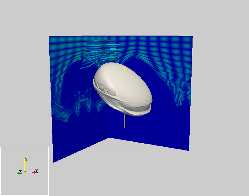
Supplementary Figure 7: Simulating magnetic draping of field loops: Shown is a side view of a draping simulation where the field consisted of loops of size $\lambda=14~{}\mathrm{kpc}$. None of the loops contain the stagnation line, so they are simply swept individually around the galaxy, experiencing only modest stretch; no significant draping occurs (field lines and cut planes are coloured by magnetic energy density using the same colour scale as in Fig 6.

It is worth noting that not every field configuration that formally meets the criterion of Eqn. 10 forms a coherent drape. The field also needs to meet certain morphological requirements. In Fig 6, we show our canonical galaxy model moving through a field of ‘loops’ of size $14\,\mathrm{kpc}$; the field configuration coming in through the top boundary is given by $\textbf{{B}}=B_{0}\cos(2\pi y/\lambda)\left(\sin(2\pi z/\lambda),0,\sin(2\pi x/\lambda)\right)$ where $B_{0}$ is chosen to give us $\beta=100$. Because the loops do not contain the stagnation line, they simply pass over the galaxy experiencing only modest shear and thus there is very little amplification and no draping layer is formed.

2.4 Does the draped field orientation reflect the ambient field?

To be able to make the claim that the draped field reflects the orientation (in that plane) of the ambient field, we must ensure that the field is not greatly changed by the process of draping, or at least is not reoriented by significantly more than existing uncertainties. This can be tested by examining our simulations, as well as in observations of draping in other environments.

In considering draping of the Solar wind over the Earth, recent work[2005AnGeo..23..885C] comparing the instantaneous ambient solar wind field to the draped field over the earth found ‘perfect draping’, that is a draped field within $10$ degrees of the solar wind field, approximately 30% of the time; the remaining time the draped field orientation remained within $30$ degrees of the ambient field. This is already promising, as the Earth’s magnetospheric system is much more complicated and rapidly changing than the system we are considering; the Earth’s tilted dipole rotates once per day, the solar wind field changes on still shorter timescales, and imperfect ionisation of the medium means that reconnection between these two very dynamic sources of field plays an important role, particularly at the bottom boundary of the drape. The upper boundary, however, we would expect to remain unchanged.

While we don’t expect such dynamics in the physical system considered here, there is however an added hydrodynamic effect; because of the reduced symmetry compared to draping over a sphere, the flow is not symmetric. At the stagnation point, flow lines separate into lines going down along the diameter of the galaxy and into lines going along the side, dragging field lines with them. This can tend to drag intermediate field lines towards alignment with the plane containing the galaxy normal and the direction of motion of the galaxy.

As shown in Fig. 8, for field twists of 45 and 60 degrees, we see only modest (at most $15$ degrees of rotation) effects; and most crucially, it is quite monotonic, and therefore predictable and can be corrected for. The difference is largest for intermediate angles; for fields nearly aligned with the direction of stretch, the effect is not important, and for field lines nearly orthogonal to the effect, the effect is extremely small. Further, because the flow follows a known pattern, the bending of the field lines has a characteristic signature with its magnitude growing then decreasing across the face of the galaxy. This pattern is transverse to the flow, so cannot be confused with a polarisation twist due to field changes in the direction of motion of the galaxy.

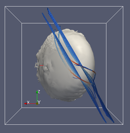
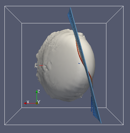
Supplementary Figure 8: Intermediate field ‘tilts’ and reorientation: Shown are views from the top (that is, from the direction of the wind felt by the galaxy) of two simulations run with field tilts intermediate to those of the field configurations shown in Fig. 2 of the main body. As shown in the streamlines of the 3D renderings in Fig. 4 of the main body, the flow over the front of the galaxy is pulled over the diameter of the galaxy; this leads to some modest field reorientation, shown here.

We also note that this field adjustment varies with galaxy orientation relative to its direction of motion. For galaxies moving face-on through the ICM, symmetry prevents any reorientation. For galaxies moving edge-on, the effect would be maximal, but measuring the magnitude of the effect will require simulations with more realistic galaxy models.

On the basis of these measurements, then, we can see that field lines nearly orthogonal to the plane connecting the galaxy normal and direction of motion (in the coordinate system used here, this means field lines near the $z$-coordinate direction) do not get significantly reoriented; neither do field lines draped over a nearly face-on galaxy. Field lines near a 45-degree angle to the plane connecting the normal to the direction of motion can be reoriented by about $15$ degrees in a predictable (and thus correctable) way; however in our current sample of galaxies we do not have any of these cases.

2.5 Magnetic field components in the direction of motion

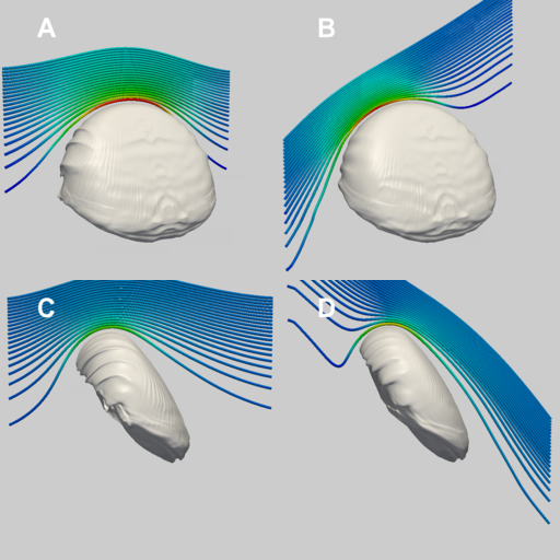
Supplementary Figure 9: Field component in direction of motion: Shown are views from four simulations of a galaxy with a 60 degree inclination towards the direction of motion moving into a uniform magnetic field. In panel A the field is oriented in the $z$-direction, and in panel B, the same magnitude field is given an equal component along the $y$ direction, the direction of motion. Similarly, in panel C, the field is oriented in the $z$ direction, whereas in D that same field now also has a component in the direction of motion. In both cases B and D, the position of the peak magnetic field strength in the drape is shifted away from the hydrodynamic stagnation point; the magnetic field ‘hot spot’ will now not be co-located with the HI ram-pressure induced hot spot. This direction-of-motion asymmetry is a sign that the field the galaxy is moving into has a significant component along the direction of motion.

Does the location of the maximum value of the magnetic energy density in the drape, $\textbf{{x}}(B_{\mathrm{max,~{}drape}})$, always coincide with the stagnation point? In contrast to $\textbf{{x}}(B_{\mathrm{max,~{}drape}})$, the stagnation point is a direct observable as the ram pressure causes the neutral gas – as traced by the HI emission – to be moderately enhanced at the stagnation point which results in an ‘HI hot spot’. Hence this question addresses a potential bias of the morphology of the polarised intensity with respect to the direction of motion.

Let’s first look at the two extreme cases: (1) a homogeneous magnetic field perpendicular to the galaxy’s direction of motion and (2) a field that is aligned with the galaxy’s proper motion. In the first case, $\textbf{{x}}(B_{\mathrm{max,~{}drape}})$ coincides with the stagnation point as this is the point of first contact with an undistorted field line. In the latter case, draping is absent as the galaxy smoothly distorts the field lines and causes a minor enhancement of the magnetic energy density around the equator with respect to the vector of proper motion. For any arbitrary field angle in between these two cases (with a field component in direction of motion), we expect $\textbf{{x}}(B_{\mathrm{max,~{}drape}})$ to be perpendicular to the local orientation of the magnetic field in the upstream as this is the point of first contact with an undistorted field line. This ‘direction-of-motion asymmetry’ is clearly demonstrated in Fig. 9 and has to be corrected for when estimating the upstream orientation of the magnetic field.

2.6 Kelvin-Helmholtz instability

We expect the contact boundary layer between these galaxies and the ICM to become unstable to shearing motions on time scales less than the orbital crossing time of these galaxies $\tau_{\mathrm{cross}}\simeq 2\,R_{\mathrm{cluster}}/\upsilon_{\mathrm{gal}}\simeq 2$ Gyr. In the absence of gravity, the growth rate of this Kelvin-Helmholtz instability is given by[chandra]

$$\omega_{\mathrm{KH}}=k\,\Delta\upsilon\,\frac{\sqrt{\rho_{\mathrm{ism}}\,\rho_{\mathrm{icm}}}}{\rho_{\mathrm{ism}}+\rho_{\mathrm{icm}}}\simeq\frac{3\pi\,\upsilon_{\mathrm{gal}}}{\lambda}\,\sqrt{\frac{\rho_{\mathrm{icm}}}{\rho_{\mathrm{ism}}}}\simeq\frac{3\pi\,c_{\mathrm{ism}}}{\lambda}.$$ (13)

Here we used the maximum shear velocity of the potential flow solution in the absence of a magnetic field[2008ApJ...677..993D], $\Delta\upsilon=1.5\,\upsilon_{\mathrm{gal}}$, and energy conservation at the interface, $\rho_{\mathrm{ism}}\,c_{\mathrm{ism}}^{2}=\rho_{\mathrm{icm}}\,\upsilon_{\mathrm{gal}}^{2}$. It turns out that the self-gravity of the disk has a negligible effect on stabilising the interface. Hence the interface becomes unstable to the shear on a timescale

$$\tau_{\mathrm{KH}}\simeq\frac{2}{3}\,\frac{\lambda}{c_{\mathrm{ism}}}\simeq 0.5~{}\mathrm{Gyr}\,\frac{\lambda}{10\mbox{ kpc}}.$$ (14)

Even though the multi-phase structure of the ISM could provide some stabilising viscosity, we still expect the small scales to become unstable on timescales much less than an orbital crossing time of the cluster in the absence of a stabilising agent such as magnetic tension in the magnetic draping layer in the direction of the field[2007ApJ...670..221D].

3 Modelling cosmic ray electrons

Our MHD simulations of a projectile moving through the intracluster magnetic field self-consistently models the magnetic field distribution in the contact boundary layer between the galaxy and the ICM. The observable synchrotron radiation, however, requires modelling a second ingredient – high energy electrons or cosmic ray electrons (CRes) which are accelerated by the field, thus emitting radiation at a characteristic frequency[RybickiLightman]

$$\nu_{\mathrm{sync}}=\frac{3eB}{2\pi\,m_{\mathrm{e}}c}\,\gamma^{2}\simeq 5\mbox{ GHz}\,\frac{B}{7\,\mu\mbox{G}}\,\left(\frac{\gamma}{10^{4}}\right)^{2},$$ (15)

where $e$ denotes the elementary charge, $c$ the speed of light, $m_{\mathrm{e}}$ the electron mass, and the particle kinetic energy $E/(m_{\mathrm{e}}c^{2})=\gamma-1$ is defined in terms of the Lorentz factor $\gamma$. In the draping layer, these electrons cool on a synchrotron timescale of

$$\tau_{\mathrm{sync}}=\frac{E}{\dot{E}}=\frac{6\pi m_{\mathrm{e}}c}{\sigma_{\mathrm{T}}B^{2}\gamma}=5\times 10^{7}\,\mathrm{yr}\,\left(\frac{\gamma}{10^{4}}\right)^{-1}\left(\frac{B}{7\,\mu\mathrm{G}}\right)^{-2}$$ (16)

where $\sigma_{\mathrm{T}}$ is the Thomson cross section. In the absence of a magnetic field, we can derive an upper limit on the cooling time by considering inverse Compton interactions of these CRes with the photons of the cosmic microwave background, yielding

$$\tau_{\mathrm{ic}}=\frac{6\pi m_{\mathrm{e}}c}{\sigma_{\mathrm{T}}B_{\mathrm{cmb}}^{2}\gamma}=2\times 10^{8}\,\mathrm{yr}\,\left(\frac{\gamma}{10^{4}}\right)^{-1},$$ (17)

where we use the equivalent magnetic field strength of the energy density of the CMB at redshift $z=0$, $B_{\mathrm{cmb}}=3.24\,\mu\mbox{G}$.

3.1 Origin of cosmic ray electrons

We now turn to the question about the source of the CRes. There are two possibilities – they could either come from the ICM, or from within the interstellar medium of the galaxy itself. We will show that the first possibility is inconsistent with the observations by discussing three detailed models, namely injection by a population of multiple active galactic nuclei, shock acceleration ahead of the galaxies, and turbulent re-acceleration of an aged population of CRes. 1) Since these electrons have very short cooling timescales they would have to be injected at a distance $L<\tau_{\mathrm{ic}}\upsilon_{\mathrm{gal}}\simeq 240$ kpc ahead of the galaxy using $\upsilon_{\mathrm{gal}}\simeq 1000\,\mathrm{km/s}$, and possibly much closer when considering non-zero magnetic fields within the ICM. However we neither observe the radio lobes of the AGN or starburst driven winds nor strong intra-cluster shocks that would be responsible for the injection of CRes. Also the published values of the radio spectral index at the stagnation point of the polarisation ridge[2004AJ....127.3375V] with $\alpha_{\nu}=0.7$ are consistent with a freshly injected CRe population similar to that observed in our Galaxy. This would be difficult to arrange with a causally unconnected process in the ICM which had to be in the immediate vicinity of all these galaxies. 2) Since these galaxies orbit trans-sonically, we can safely assume that their velocities never exceed twice the local sound speed yielding a Mach number constraint of ${\mathcal{M}}<2$. Adopting the standard theory of diffusive shock acceleration in the test particle limit[1987PhR...154....1B], we can relate the spectral index $p$ of the accelerated CR distribution to the density compression factor $R$ at the shock through $p=(R+2)/(R-1)$. Adopting the well known Rankine-Hugoniot jump conditions and using $\Gamma=5/3$, we arrive at[2007A&A...473...41E]

$$p=\frac{4+{\mathcal{M}}^{2}(3\Gamma-1)}{2({\mathcal{M}}^{2}-1)}>3.3,\mbox{ for }{\mathcal{M}}<2.$$ (18)

Hence the synchrotron spectral index $\alpha_{\nu}=(p-1)/2>1.15$ of such a shock-accelerated population of CRes would be inconsistent with the observations[2004AJ....127.3375V]. 3) Re-acceleration processes of ‘mildly’ relativistic electrons ($\gamma\simeq 100-300$) that are being injected over cosmological timescales into the ICM by sources like radio galaxies, structure formation shocks, or galactic winds can provide an efficient supply of highly-energetic CR electrons. Owing to their long lifetimes of a few times $10^{9}$ years these ‘mildly’ relativistic electrons can accumulate within the ICM[1999ApJ...520..529S], until they experience continuous in-situ acceleration either via interactions with magneto-hydrodynamic waves, or through turbulent spectra[1977ApJ...212....1J, 1987A&A...182...21S, 2001MNRAS.320..365B, 2002ApJ...577..658O, 2004MNRAS.350.1174B, 2007MNRAS.378..245B]. This acceleration process produces generically a running spectral index with a convex curvature[1987A&A...182...21S, 2001MNRAS.320..365B] which is not observed in these polarisation ridges. Secondly, this process would predict an ubiquitous CRe distribution that should light up the entire magnetic drape which is not observed. In fact, the non-observation of this emission limits the efficiency of this process! Finally, the universality of the ratio of total-to-polarised synchrotron intensity[Vollmer2009] $TI/PI\simeq 10$ in these galaxies suggests a galactic source of these CRes and would again require a fine-tuning of the available turbulent energy density everywhere in the ICM – in contrast with theoretical expectations[2006PhPl...13e6501S].

Having argued against the ICM as a source of these CRes, we now consider the possible sources of CRes within the ISM. We know that the sources of CRes in our Milky Way are supernova remnant shocks[1999ApJ...525..357S, 2006ApJ...648L..33V] as well as hadronic reactions of CR protons with ambient gas protons[2006Natur.439..695A]. Are the CRes that are injected deeply inside the gas disk able to diffuse through the galaxy and populate the entire magnetic drape? As we saw in Fig. 2, the process of magnetic draping causes the field lines to become aligned with the contact discontinuity. This implies that the CRe that enter the draping sheath from inside the galaxy gyrate the innermost field lines with a Larmor radius of

$$r_{\mathrm{L}}=\frac{p_{\bot}c}{eB}\simeq 10^{-6}\,\mathrm{pc}\,\frac{\gamma}{10^{4}}\left(\frac{B}{7\,\mu\mathrm{G}}\right)^{-1}.$$ (19)

The diffusion process in such a low-collisionality plasma perpendicular to the field lines is suppressed by a factor of order $10^{12}$ relative to the Spitzer value[2003A&A...399..409E] and makes it impossible for these CRes to efficiently populate the drape.

As explained in the text, there is a mechanism that accelerate CRes directly within the draping layer: The ram pressure that the galaxy experiences in the ICM displaces and strips some of the outermost layers of gas in the galaxy, but the stars are largely unaffected. Thus the stars lead the galactic gas at the leading edge of the galaxy at which the magnetic draping layer forms. As these stars become supernovae, they drive powerful shock waves into the ambient medium that accelerates electrons to relativistic energies. Assuming a conservative supernova rate of one per century, the number of supernova events above one galactic scale height within $\tau_{\mathrm{syn}}$ is given by

$$N_{\mathrm{sn}}=\frac{\tau_{\mathrm{syn}}}{\tau_{\mathrm{sn}}}=\frac{5\times 10^{7}\,\mathrm{yr}}{2\,e\,100\,\mathrm{yr}}\simeq 10^{5}.$$ (20)

Consider the supernova that dumps its energy $E_{\mathrm{sn}}\simeq 10^{51}$ erg explosively into the surrounding gas. After an initial phase of free expansion, there will be a second phase when the nuclear energy of the explosion drives a self-similar strong shock wave into the ambient medium (the so-called Sedov solution). We are interested in the maximum radius of such a remnant shock as it determines the homogeneity of the resulting CRe distribution when considering an ensemble of supernova explosions within a synchrotron cooling time. The condition for the shock phase is such that the energy deposited by the supernova has to be larger than the sum of internal energy and ram pressure times the shock volume of the ambient medium (neglecting radiative losses throughout this process), or

$$E_{\mathrm{sn}}\stackrel{{\scriptstyle!}}{{>}}\frac{4}{3}\pi R_{\mathrm{sn}}^{3}(\varepsilon_{\mathrm{icm}}+\rho_{\mathrm{icm}}\upsilon_{\mathrm{gal}}^{2}).$$ (21)

Using a typical velocity for the galaxy of $\upsilon_{\mathrm{gal}}\simeq 1000\,\mathrm{km/s}$, and a gas of primordial element abundance in Virgo with $n_{\mathrm{icm}}\simeq 10^{-4}\,\mathrm{cm}^{-3}$ and $kT\simeq 6.7$ keV, we compute a maximum shock radius of $R_{\mathrm{sn}}=150$ pc. It turns out that the maximum radius for supernovae exploding inside the galaxy, but in the immediate vicinity of the contact will be exactly the same as the ISM reacts to the ram pressure and slightly increases its density. It is now straight forward to calculate the filling factor of supernova remnant shocks in the region where the stellar disk intersects the magnetic draping layer, yielding

$$f_{\mathrm{sn}}=\frac{N_{\mathrm{sn}}\pi R_{\mathrm{sn}}^{2}}{\pi R_{\mathrm{gal}}^{2}}\simeq 6,$$ (22)

where we adopted $R_{\mathrm{gal}}\simeq 20$ kpc. This implies that multiple supernova remnants intersect each other which leads to a smooth distribution of CRes, consistent with what we observe in our Galactic synchrotron emission[2009ApJS..180..265G]. It follows that the CRes can maintain a smooth distribution that follows that of the star light.

3.2 Spatial distribution

As these CRes are injected in a homogeneous manner, their steady state distribution within the draping layer is governed by transport and cooling processes. Since these CRe are largely constrained to stay on any given line, and this field line is ‘flux-frozen’ into the medium, it is advected with the ambient flow over the galaxy leading to an advection length scale of $L_{\mathrm{adv}}\simeq 10\,\mathrm{kpc}$ as described in the text. The CRes interact with Alfvén waves that cause them to random walk along that field line. Hence the distribution along these field lines can be described by a diffusive process with a characteristic length scale from the injection region,

$$L_{\mathrm{diff}}=\sqrt{2\kappa\tau_{\mathrm{sync}}}=6\,\mathrm{kpc}\,\left(\frac{\kappa}{10^{29}\,\mathrm{cm}^{2}\,\mathrm{s}^{-1}}\right)^{1/2}.$$ (23)

These considerations detail the spatial extent of the CRe distribution that emits high-frequency (4.85 GHz) radio synchrotron emission. How do we normalise their number density? Simulating all-sky maps in total intensity, linear polarisation, and Faraday rotation measure for the Milky Way, the CRe distribution has been derived to be exponential both in cylindrical radius from the centre and height above the mid-plane of the galaxy[2008A&A...477..573S, 2009A&A...495..697W]

$$n_{\mathrm{cre}}=C_{0}\,e^{-(R-R_{\odot})/h_{R}}e^{-|z|/h_{z}}$$ (24)

with the radial scale ‘height’ $h_{R}\simeq 8\,\mathrm{kpc}$, the $z$ scale height corresponding to the thick disk height $h_{z}\simeq 1\,\mathrm{kpc}$, and $C_{0}$ a normalisation chosen to give representative CRe densities at the Solar position, $C_{0}\simeq 10^{-4}\,\mathrm{cm}^{-3}$. In our Galaxy, all three components, gas, magnetic fields, and CR protons are in equipartition with an energy density of about 1 eV per cm³. The energy density of CRes is a factor of 100 below that due to properties of electromagnetic acceleration processes and the fact that CRe become relativistic at much smaller energies compared to protons[2002cra..book.....S].

It is a non-trivial task to map this CRe distribution and its normalisation from our Galaxy to Virgo cluster spirals. To this end we employ the far-infrared (FIR)-radio correlation of these galaxies and compare it to typical parameters for our Galaxy in order to determine whether we would need to rescale the CRe normalisation. As already mentioned earlier, the total synchrotron intensity dominates over the polarised intensity which strongly suggests that star forming regions are the primary source of the total synchrotron emission since the turbulence – perhaps induced by supernova explosions – destroys the large scale interstellar magnetic field and causes depolarisation of the intrinsically polarised emission. Hence the star formation rate is also expected to strongly correlate with the overall spatial distribution of CRes in these galaxies. We use the surface density of gas, $\Sigma_{\mathrm{gas}}$, as a proxy of the star formation rate[1998ApJ...498..541K] and find $\Sigma_{\mathrm{gas}}\simeq 2.5\times 10^{-3}\mathrm{g\,cm}^{-2}$ in five galaxies out of our sample of eight where we had data available for this comparison. This agrees exactly with $\Sigma_{\mathrm{gas}}$ at the solar circle of our Galaxy[2006ApJ...645..186T]. Since the radio luminosity depends on the uncertain emission volume, we decided to use the minimum energy magnetic field strength[1994hea..book.....L] as a robust measure of the energy density in magnetic fields and CRes. Except for NGC 4548, we find values of $B_{\mathrm{min}}\simeq(5\ldots 8)\,\mu$G which again agrees very well with the Galaxy’s value at the solar circle of $B_{\mathrm{min}}\simeq 6\,\mu$G[2001SSRv...99..243B]. In fact, the low value of NGC 4548, $B_{\mathrm{min}}\simeq 2.3\,\mu$G could indicate a lower normalisation of the CRe distribution which would be a natural explanation of the weakness of the observed polarised emission.

For this work, we decide to use a two-step phenomenological model in the post-processing step and postpone a dynamical model of the transport of CRes to future work[D&P]. 1) We use the CRe distribution of an undisturbed galaxy of Eqn. 24 ‘inside’ our model galaxy. The centre of mass of our galaxy is found, and the orientation of the galaxy at time zero is used to determine the mid-plane. (The much more massive galactic gas is never measurably re-oriented during the course of this simulation.) Because our model galaxy is thicker for numerical reasons than the aspect ratio implied with the scale heights above (our aspect ratio for the galaxy is 10:1 rather than the 20:1 given by $R:h_{z}$) we used $h_{z}=2\,\mathrm{kpc}$; thus the cosmic ray number density has fallen off by one factor of $e$ by the top of the model galaxy.

2) In a second step, the exponential profiles are truncated at the contact discontinuity between the galaxy and the ICM – e.g., corresponding to the initial unperturbed cosmic-ray containing gas in the outer regions of the galaxy being efficiently stripped away. Instead, we attach another exponential distribution of CRes perpendicular to the 3D surface of the contact outside the galaxy while requiring a continuous transition of the CRe distribution from within the galaxy. This setup mimics the CRe acceleration by supernovae in the draping region where the stars lead the ram pressure displaced interstellar gas as well as subsequent advective and diffusive transport processes of the CRes around the galaxy. We choose the scale height to be of the characteristic size of a supernova remnant (Eqn. 21) and leave the specific value $h_{\bot}\simeq(150\ldots 250)$ pc of this exponential as a free parameter that will be explored in Sect. 4.3.

In detail, the contact discontinuity between the galaxy and the ICM is determined by a density and magnetic field cutoff; the magnetic field is zero within the galaxy and the density is low outside of the galaxy, i.e. $\rho<\rho_{c}$ or $|B|>B_{c}$, where $\rho_{c}$ and $B_{c}$ are cutoff values chosen to reproduce the contact discontinuity. Any suitably small value of the magnetic cutoff was seen to correctly separate the upper part of the galaxy from the ICM. The implied location of the contact discontinuity was much more sensitive to the density cutoff; after trial and error, this value was chosen to be approximately 40% above the ambient density, $\rho_{c}=1.4$. The ICM density is seen to drop to below the ambient value in the draping layer, increasing the contrast; and no shocks occur above the galaxy, meaning there is no compressive density enhancement to values above this to confuse galactic material with shock-compressed ICM material. A further cutoff is placed so that no cosmic rays exist at $3~{}\mathrm{kpc}$ below the galactic mid-plane or beyond; this ensures that no stripped galactic material in the wake is allowed to ‘light up’. Dense stripped material travels quite slowly (approximately 1/10th or less the speed of the ICM ‘wind’) and the flow lines around the galaxy increase the flow time of the stripped material to $\tau>5\times 10^{7}\,\mathrm{yr}$ to be advected that far below the galaxy; at this time, the cosmic rays would have already cooled to the point that they would not emit significant amounts of synchrotron radiation at high radio frequencies.

4 Modelling the synchrotron emission

4.1 Formulae and algorithms

Here we summarise the equations for calculating the maps of the polarised synchrotron emission. The synchrotron emissivity (power per unit volume, per frequency, and per solid angle) is partially linearly polarised. In the limit of ultra-high energy CRes with $\gamma\gg 1$, the synchrotron polarisation and intensity depends on the transverse component of the magnetic field, $B_{\mathrm{t}}=B_{\mathrm{t}}(\textbf{{x}})$ (perpendicular to the line-of-sight), as well as on the spatial and spectral distribution of CRes. The emissivities $j_{\bot,\|}=\mathrm{d}^{4}E_{\bot,\|}/\mathrm{d}t\,\mathrm{d}\omega\,\mathrm{d}\Omega\,\mathrm{d}V$, perpendicular and parallel to $B_{\mathrm{t}}$ are given by[RybickiLightman]

$$j_{\bot,\|} = \frac{1}{4\pi}\frac{\sqrt{3}\,e^{3}}{8\pi m_{\mathrm{e}}c^{2}}\left(\frac{2m_{\mathrm{e}}c\omega}{3e}\right)^{\frac{1-p}{2}}CB_{\mathrm{t}}^{\frac{p+1}{2}}\Gamma\left(\frac{p}{4}-\frac{1}{12}\right)$$ (25)

$$\times \left[\frac{2^{\frac{p+1}{2}}}{p+1}\Gamma\left(\frac{p}{4}+\frac{19}{12}\right)\pm 2^{\frac{p-3}{2}}\Gamma\left(\frac{p}{4}+\frac{7}{12}\right)\right].$$

Here $C=C(\textbf{{x}})$ denotes the normalisation of the CRe distribution and is defined by $N(\gamma)\mathrm{d}\gamma=C\gamma^{-p}\mathrm{d}\gamma$, $N(\gamma)$ the number density of CRes $\in[\gamma,\gamma+\mathrm{d}\gamma]$, $p=2\alpha_{\nu}+1=2.4$ is the spectral index that we fix by considering the observed synchrotron spectral index $\alpha_{\nu}=0.7$ at the stagnation point[2004AJ....127.3375V], and $\omega=2\pi\nu$, where $\nu$ is the observational frequency. Denoting the angular position on the sky by a unit vector $\hat{\textbf{{n}}}$ on the sphere, the polarised specific intensity $P=P(\omega,\hat{\textbf{{n}}})$ can be expressed as a complex variable (cf. reference[1966MNRAS.133...67B]),

$$P(\omega,\hat{\textbf{{n}}})=\int_{0}^{L}\mathrm{d}r\left[j_{\bot}(\omega,\hat{\textbf{{n}}})-j_{\|}(\omega,\hat{\textbf{{n}}})\right]\mathrm{e}^{2i\chi(r,\hat{\textbf{{n}}})}.$$ (26)

A process called Faraday rotation arises owing to the birefringent property of magnetised plasma causing the plane of polarisation to rotate for a nonzero magnetic field component along the propagation direction of the photons. The observed polarisation angle $\chi$ is related to the source intrinsic polarisation angle $\chi_{0}$ (orthogonal to the magnetic field angle in the plane of the sky) through

$$\chi(r,\hat{\textbf{{n}}}) = RM(\hat{\textbf{{n}}})\,\lambda^{2}+\chi_{0}(\hat{\textbf{{n}}})$$ (27)

$$RM(\hat{\textbf{{n}}}) = a_{0}\int_{0}^{L}B_{r}(\textbf{{x}})\,n_{\mathrm{e}}(\textbf{{x}})\,\mathrm{d}r$$ (28)

$$\simeq 812\,\frac{\mathrm{rad}}{\mathrm{m}^{2}}\,\frac{B}{\mu G}\,\frac{n_{\mathrm{e}}}{10^{-3}\mbox{ cm}}\,\frac{L}{\mbox{Mpc}},$$ (29)

where $a_{0}=e^{3}/(2\pi m_{\mathrm{e}}^{2}c^{4})$ and $n_{\mathrm{e}}$ is the number density of electrons. In the last step, we assumed constant values and a homogeneous magnetic field along the line-of-sight to give an order of magnitude estimate for $RM$ values. The Stokes $Q$ and $U$ parameters correspond to the real and imaginary components of the polarised intensity and are the integrals over solid angle,

$$Q+iU=\int\mathrm{d}\Omega\,P.$$ (30)

We discretise the equations above, rotate the simulation volume to the desired viewing angle, and sum up the individual Stokes $Q$ and $U$ parameters of each computational cell to obtain the line-of-sight projection. From the integrated Stokes parameters we obtain the magnitude of the polarisation $|P|=\sqrt{Q^{2}+U^{2}}$ and the polarisation angle $\chi=0.5\,\arctan(U/Q)$. This enables us to infer the orientation of the magnetic field in the draping layer which is identical to the direction of the polarisation vectors rotated by 90 degrees and uncorrected for Faraday rotation (hereafter referred to as ‘B-vectors’).

4.2 Faraday rotation

It turns out that Faraday rotation from within the drape can be safely ignored, since an order of magnitude estimate yields a negligible rotation of the plane of polarisation with

$$\Delta\chi\simeq 0.01\deg\,\left(\frac{\lambda}{\mathrm{6\,cm}}\right)^{2}\,\frac{B_{\mathrm{drape}}}{7\,\mu\mathrm{G}}\,\frac{n_{\mathrm{e}}}{10^{-4}\mbox{ cm}^{-3}}\,\frac{L_{\mathrm{drape}}}{100\mbox{ pc}}.$$

How does the Faraday rotation of the ICM bias the inferred magnetic field direction? Since the gradient of the ICM density and magnetic field strength across the galaxies’ solid angle is negligible, we expect a coherent rotation of all polarisation angles. Using typical values from deprojected Virgo X-ray profiles (see Fig. 15), we estimate the magnitude of the overall rotation for a line-of-sight that does not intersect the Virgo core region to

$$\Delta\chi\simeq 2\deg\,\left(\frac{\lambda}{\mathrm{6\,cm}}\right)^{2}\,\frac{B_{\mathrm{icm}}}{0.1\,\mu\mathrm{G}}\,\frac{n_{\mathrm{e}}}{10^{-4}\mbox{ cm}^{-3}}\,\frac{L_{\mathrm{cluster}}}{1\mbox{ Mpc}}.$$

This is small enough not to bias our inferred magnetic field direction. The adopted parameters for the ICM outside the dense cluster core regions imply an $RM\simeq 8~{}\mathrm{rad/m}^{2}$ which is also much smaller than the measured $RM$ values towards central radio lobes. Hence this explains why the radial field structure that we find in this work has not yet been measured in the $RM$ statistics from radio lobes. Using polarised sources with a large angular extent such as radio relics[2009MNRAS.393.1073B], future low-frequency radio interferometers (GMRT, LOFAR, MWA, LWA) should be able to detect this field geometry.

4.3 Parameter study

In Fig 10 we see the effects for one of our runs (the same simulation and orientation as shown on the right hand side of Fig. 2 in the main body) as we vary our distribution of CRe outside of the galaxy. The relevant scale for these cosmic rays from supernovae should be something of the order 300 pc, corresponding to a 150 pc radius for a typical supernova remnant under these conditions as described above. We plot the resulting polarised synchrotron radiation for cases with a cosmic ray distribution with scale heights 0.1, 150, 200, and 250 pc. Because the synchrotron intensity varies linearly with the CRe number density but roughly quadratically as the magnetic field, and the magnetic field energy density is extremely sharply peaked ($B^{2}~{}s^{-1}$, cf. Eqn. 2) at the contact discontinuity, it is the magnetic field which is most important in setting the morphology of the region of synchrotron emission, and adjusting the scale height of the cosmic ray distribution primarily changes the overall normalisation. Further, since we are modelling our distribution as an exponential tail times the nearest galactic value, we very quickly hit diminishing returns; once the draped region is fully populated (e.g., the scale height is several times the drape thickness, 88 pc in our fiducial simulation case) then further increases in scale height do little to increase the synchrotron emission.

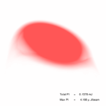
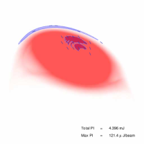
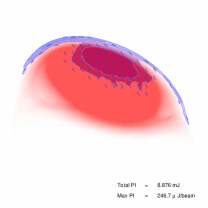
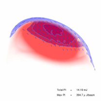
Supplementary Figure 10: Parameter study of cosmic ray distribution scale height. Parameter study on varying the cosmic ray scale height out of the galaxy. Shown is a projection through the simulation volume for our fiducial $\textbf{{B}}=B_{o}\hat{\textbf{{x}}}$ case of density (red), synchrotron polarised intensity (blue contours), and inferred magnetic field angle (lines) Compare are the cases with a tiny scale height (scale height = $0.1\,\mathrm{pc}$), top left; one with somewhat smaller height than used in this work (scale height = $150\,\mathrm{pc}$), top right; with our default value (scale height = $200\,\mathrm{pc}$, bottom left); and with a larger one (scale height = $250\,\mathrm{pc}$, bottom right. Contours are fixed to to those used in recent observational work on Virgo cluster spirals[Vollmer2008]. The extra-galactic scale height of the exponential distribution of CRes effects the overall normalisation of the observed polarised intensity but does not alter the morphology seen.

We choose 200 pc as a fiducial scale height for modelling our cosmic ray distribution through the draped region, and use it through the body of this work. It is entirely possible that the true cosmic ray distribution will fall off much more slowly than this, particularly at the leading edge of the galaxy where are large stellar population exists beyond the ICM/ISM boundary. With larger values, however, our approach of adding the distribution everywhere over the galaxy is too simplistic to fully account for the realistic modelling of the transport of these cosmic rays through the draped layer by advection and diffusion. It may even produce unphysical results by e.g., implying transport over distances by which the cosmic rays would have cooled down to invisibility in the 6 cm radio observations. On the other hand, sizes much smaller ( e.g., less than 150 pc — the radius of a single supernova remnant, a characteristic length scale for injection cf. Eqn. 21) starts to become difficult to justify.

To get more realistic spatial distribution of polarisation intensities, future work must include both realistic gas/star separation and proper cosmic ray transport; however, we emphasise again that the magnetic field geometry sets the geometry and the region where one could expect synchrotron emission, the most intense emission must be near the stagnation point on the leading end, and the remaining physics simply determines how quickly the emission falls off throughout the rest of the drape.

4.4 Spectral ageing effects

As the CRes are injected by supernovae in the draping region where the stars lead the ram pressure displaced interstellar gas, they are subsequently transported advectively around the galaxy alongside the magnetic field and their distribution is smoothed out along the field lines through diffusion. Hence we expect the freshly accelerated CRes to show a spectral index of $p\simeq 2.3$, similar to what we observe at supernova remnants in our Galaxy. As they cool radiatively, their spectrum steepens so that we expect a larger spectral index as we move towards the edges of the polarised synchrotron ridge (to be modelled in future work[D&P]). There we expect to probe either a simply ageing CRe population or observe a superposition of an aged CRe population and freshly injected CRes with a decreasing number density there as the ram pressure component normal to the gas decreases for a given inclination of the galactic disk (due to a smaller region of displacement of stars and the disk). This exact behaviour is in fact observed along the polarised ridge in NGC 4522[2004AJ....127.3375V, 2009ApJ...694.1435M]. This is a universal prediction of our model!

5 Bringing it together: magnetic draping and synchrotron polarisation

In order establish an intuition of the physics of magnetic draping at galaxies as well as the resulting radio polarisation we contrast 3D volume renderings of our simulations and the mock polarisation maps in the following. We will vary the galactic inclination, the tilt of the cluster magnetic field, and the viewing angle separately.

5.1 Varying the galactic inclination

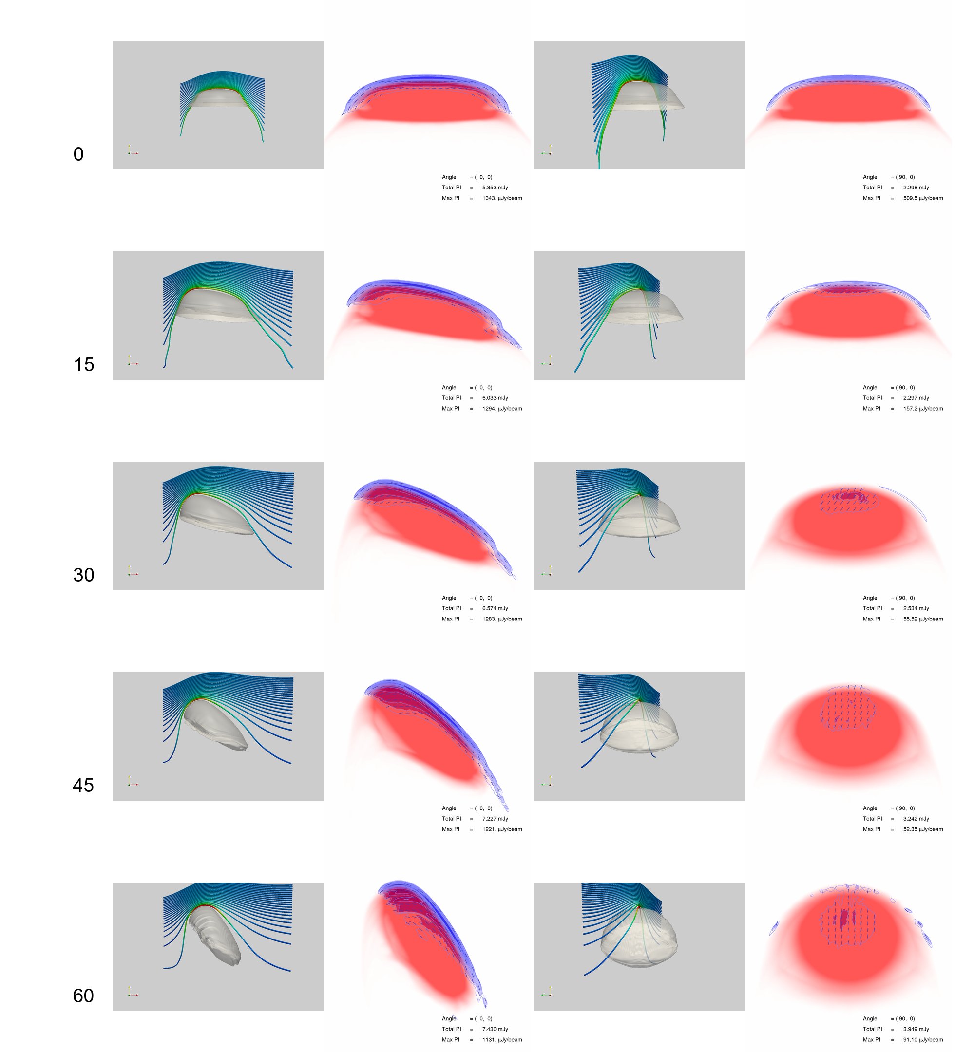
Supplementary Figure 11: 3D Renderings and polarised synchrotron radiation for models of different inclination. For five different simulations of galaxies with different inclinations moving upwards into a homogeneous magnetic field of a fixed orientation (30 degrees from the $z$-direction towards the $x$-direction), we see 3D renderings and simulated polarised synchrotron emission views from two points of view – along the $z$ axis (left) and $x$ axis (right). Note that in this case peak polarised intensity is much greater viewed ‘edge on’ than ‘face on’. The reason for this is that one observes a much greater column density of polarised synchrotron emitting material as one is seeing along the drape width, of order the galaxy size; face on, one integrates only through the drape thickness at the rim. Also note that peak magnetic energy density is higher in the higher-inclination cases; as the field gets draped over a region of smaller curvature radius, it is harder to move the field off of the stagnation point, and so the steady-state field strength is greater.

In Figure 11 we show two views (edge-on, face-on) of multiple simulations with varying the galactic inclination. For the edge-on views on the left, we observe an increase of asymmetry of the polarised intensity (PI) for increasing inclination. The face-on views on the right show a decrease in PI an the stagnation point. This is due to a combination of two effects: 1) for an increase in inclination, magnetic field lines get more effectively reoriented as they are advected with the flow over the galaxy as discussed in detail in Sect. 2.4. 2) This leads to a large line-of-sight component of the magnetic field if the galaxy is viewed face-on. As the polarised synchrotron emission only maps out the transverse magnetic field component $B_{\mathrm{t}}$ (perpendicular to the line-of-sight), this effect biases the polarised emission low relative to the total magnetic energy density in the draping sheath (causing a so-called ‘geometric bias’). Within a factor of three, the magnitude of the total PI is very similar for the face-on and edge-on view. This suggests that the geometric bias only affects the polarised intensity at the rim, but not in projection across the galaxy. This is supported by the direction of the B-vectors across the galaxy that resemble the orientation of the upstream magnetic field.

Interestingly, the overall morphology of galaxy changes due to ram pressure, in particular the contact of the galaxy and the ICM becomes more susceptible to Kelvin-Helmholtz instabilities for higher inclinations. The magnetic draping layer becomes thinner for increasing inclinations of the galaxy with respect to the direction of motion[D&P] which increases the requirements for the numerical resolution that is need to resolve the layer. Our resolution study in Fig. 2 demonstrates that our simulations with an inclination of 45 degrees were just able to resolve the draping layer with our fiducial resolution discussed in Sect. 1.2. Most likely that is to lesser extend the case for higher inclination cases causing the Kelvin-Helmholtz instability to modify the interface of the galaxy with the ICM. The enhanced instability for high-inclination cases might also partly be an artifact of our numerical modelling of the galaxy that neglects the detailed physics (multiphase ISM including its clumpiness, self-gravity) of the interface, at least for time scales of order $10^{8}$ years that we based our analysis on. We note that these enhanced Kelvin-Helmholtz troughs that are visible in the iso-density contours also facilitate the reorientation effect of the magnetic field as flux tubes can be trapped more easily within them. The accompanying filamentary behaviour of the PI also result from this artificially enhanced effect.

5.2 Varying the tilt of the magnetic field

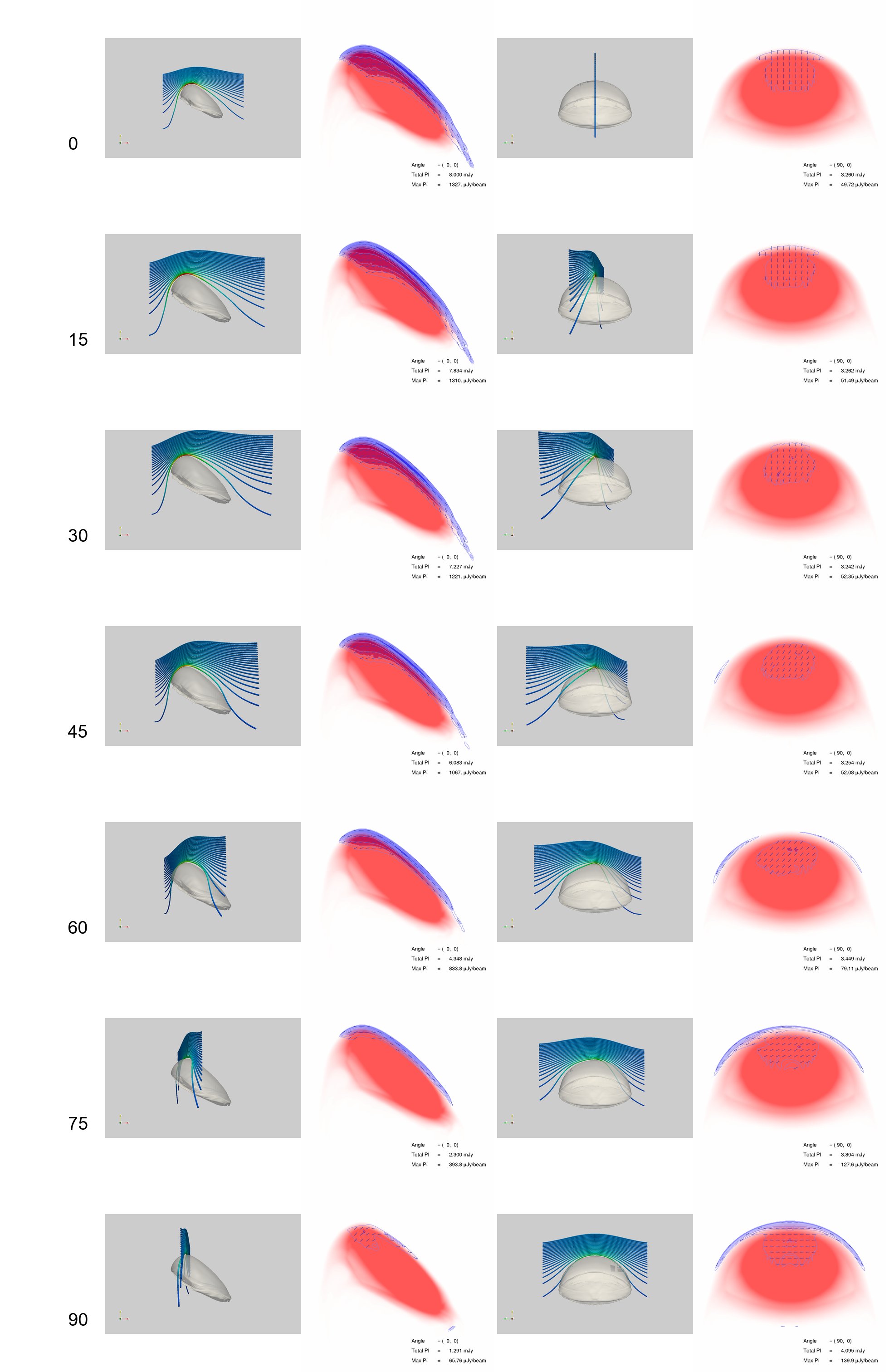
Supplementary Figure 12: 3D Renderings and polarised synchrotron radiation for models of different tilt. Shown are seven different simulations of galaxies with a fixed 45 degree inclination to the direction of motion, moving into fields with orientations ranging from along the $x$-axis (‘tilt’ of zero, top) to along the $z$ axis (‘tilt’ of ninety, bottom). On the left two columns are 3d renderings and simulated polarised synchrotron emission viewed from along the $z$ as is, and on the right, from the $x$ axis. We see the progression of polarised intensity mostly being observable when viewed from the $z$ axis to mostly being viewable when viewed from the $x$ axis.

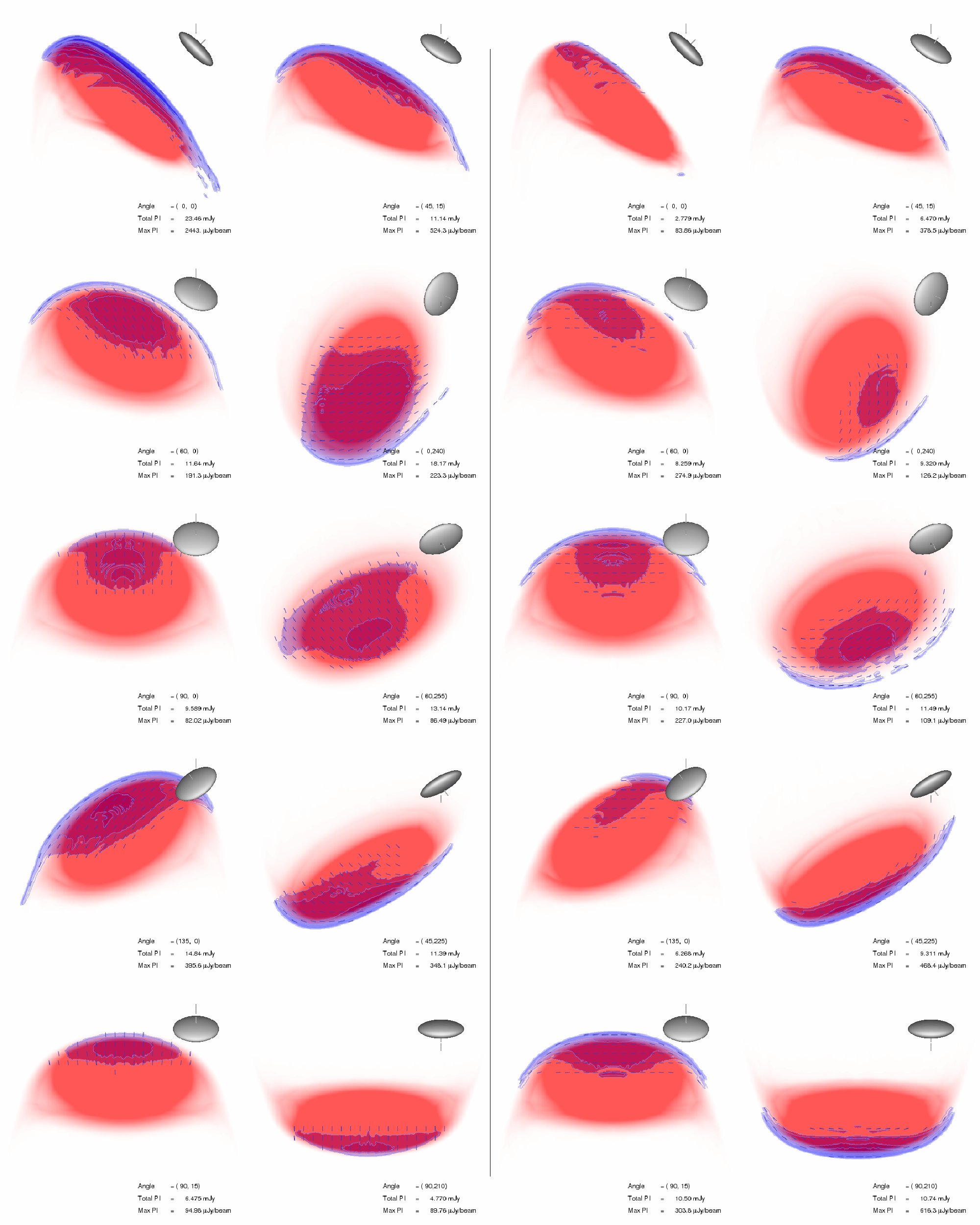
Supplementary Figure 13: Polarised synchrotron radiation of the two models shown in Fig 1 in the main paper, observed from ten different viewing angles. On the left are shown different viewpoints of the model with a homogeneous magnetic field in the $x$-direction, as in Fig 1A and 1C; on the right are the same viewpoints for the model with the magnetic field in the $z$ direction, as shown in Fig 1B and 1D. Even for a fixed model, different points of view result in a rich range of synchrotron ridge morphologies. Nonetheless, for any given viewing angle, the difference between these two very different field orientations is clearly discernable.

Figure 12 shows two views (edge-on, face-on) of multiple simulations with varying the magnetic tilt from 0 to 90 degrees. Along this sequence, the PI decreases for the edge-on view (left) and increases for the face-on view (right). The reason is again the geometric bias mentioned above. For the face-on view, this effect is accompanied with a moderate reorientation effect of intermediate tilted magnetic fields. However, the total PI remains almost unchanged - apparently it mostly impacts through the maximum value for the PI and this face-on view (which has a very small configuration space density) amplifies this effect due the high symmetry of this configuration. This makes it possible to infer ambient field orientation due to the dynamics of draping even in cases where it would be impossible to see synchrotron polarisation of an upstream B-field that is e.g., aligned with the line-of-sight. Note that there is a larger amplification of the magnetic field as well as the PI in the edge-on view due to a combination of two effects. 1) The emission region intersected by the line-of-sight is larger for the edge-on case than it is for the face-on view where it only picks up the emission from the rim. 2) The peak magnetic energy density is higher for the case of small tilts compared to the perpendicular case with a tilting angle of 90 degrees. As the field gets draped over a region of smaller curvature radius, the magnetic tension in the field is increased. More work is needed to reach steady state which results also in a higher magnetic energy density or similarly synchrotron emission. However, we caution the reader that the configuration space density is very small in both cases and particularly chosen for their high degree of symmetry that facilitates the understanding of the underlying draping physics and the resulting PI maps.

5.3 Varying the viewing angles

Figure 13 shows multiple views of two simulations of galaxies encountering a homogeneous magnetic field. It demonstrates that even in this very simple case, there is a richness of synchrotron ridge morphologies visible that clearly allows to discriminate different field geometries. In most cases, the total PI only varies within a factor of two barring very symmetric cases (that however have a small configuration space density).

6 Observational evidence and model comparison

The surprising discovery of these polarised radio synchrotron ridges poses two big questions. 1) Why does the polarised radio emission from spirals look so different from what we observe in field spiral galaxies where the polarisation is generally relatively symmetric and strongest in the inter-arm regions[2001SSRv...99..243B]? 2) What is the origin of these polarisation ridges and why are they so persistent?

The answer to the first question is straightforward as we observe the large scale magnetic field in between the dense star forming regions that constitute the spiral arms – probably caused by the strong shear in the disk. High-resolution 3D hydrodynamical simulations of the ram pressure stripping of galaxies that model the multiphase structure of the ISM self-consistently show that the lower density gas in between spiral arms is quickly stripped irrespective of its radius within the disk, while it takes more time for the higher density gas to be ablated[2009ApJ...694..789T]. Being flux-frozen into this dilute plasma, the regular large scale field will also be stripped, leaving behind the small scale field in the star forming regions. Beam depolarisation effects and superposition of causally unconnected star forming patches along the line-of-sight cause the resulting radio synchrotron emission to be effectively unpolarised.

While this work proposes a novel model to explain the second question, it is worthwhile to consider all the observational evidence[2004AJ....127.3375V, 2007A&A...464L..37V, 2007A&A...471...93W, 2009ApJ...694.1435M, 2010arXiv1001.3597V] that any model has to explain (we note that not all the characteristics in the following list have yet been studied for every galaxy in our sample).

1. The polarised radio morphology shows strongly asymmetric distributions of polarised intensity with elongated ridges located in the outer galactic disk. All edge-on galaxies with polarisation data (NGC 4388, NGC 4396, NGC 4402, NGC 4522) show extraplanar polarised emission which extends further than the HI emission.

2. The polarisation vectors are coherently aligned across the polarised ridge that often extends over entire leading edge of the galaxy over scales of $\sim 30$ kpc.

3. The distribution of stars lead the polarised emission ridge[2007A&A...464L..37V] which itself leads the HI emitting galactic gas at the leading edge of the galaxy. This is the case for all inclined galaxies (NGC 4501, NGC 4522, NGC 4654) in our sample (see Fig. 1).

4. In a few cases (most prominently at NGC 4654), we observe radio emission not just at the leading edge (as inferred from the HI morphology) but additionally at the side of the galaxy.

5. The ram pressure causes the neutral gas as traced by the HI emission to be only moderately enhanced at the stagnation point by less than a factor of two. This ‘HI hot spot’ is very localised spatially and much smaller in extent compared to the elongated polarised ridge emission.

6. The region of the ‘HI hot spot’ is almost coincident with a flat spectral index ($\alpha_{\nu}=0.7$), while $\alpha_{\nu}$ steepens towards the edges of the polarised ridge where the degree of polarisation is very large and approaching values of 40%. Most prominently this is seen in NGC 4388, NGC 4396, NGC 4402, NGC 4654[2010arXiv1001.3597V] and NGC 4522[2004AJ....127.3375V].

7. Recent work[2009ApJ...694.1435M] finds a radio-deficit region which lies just exterior to a region of high radio polarisation and flat radio spectral index, although the total 20 cm radio continuum in this region does not appear strongly enhanced. The strength of the radio deficit is inversely correlated with the time since peak pressure as inferred from stellar population studies and gas-stripping simulations, consistent with the strength of the radio deficit being a good indicator of the strength of the current ram pressure. This work also finds that galaxies having local radio deficits appear to have enhanced global radio fluxes.

8. The ratio of total-to-polarised synchrotron intensity $TI/PI\simeq 10$ in these galaxies seems to be a universal property with a maximum deviation of only 30%[Vollmer2009].

9. At the contact boundary layer between these galaxies and the ICM, there are no Kelvin-Helmholtz instabilities observed even though these interfaces should become unstable to shearing motions on time scales less than the orbital crossing time of these galaxies (Eqn. 14).

Our model of draping weak cluster magnetic fields over these galaxies is powerful enough to naturally explain all of the mentioned properties. In fact, the morphology of the polarised and total radio intensity, and the resulting degree of polarisation support the picture that the total intensity traces the star forming regions whereas the polarised intensity arises from magnetic draping of cluster fields. In particular, magnetic draping causes a thin sheath of strong fields to develop that suppresses Kelvin-Helmholtz instabilities in the direction of the field[2007ApJ...670..221D] and causes a coherent synchrotron polarisation at the leading edge of the orbiting galaxy: how exactly our model addresses points 1-5 has been explained in the main body of the paper, the issue of spectral ageing (point 6) in Sect. 4.4, and the issue of the Kelvin-Helmholtz shearing instability (point 9) in Sect. 2.6.

The flat radio spectral index indicates a freshly injected CRe population into the drape that originates from supernovae that went of just outside the drape and we do not expect to see synchrotron emission there as the magnetic field is only starting to ramp up towards the drape – hence the radio deficit relative to the stellar IR emission (point 7). The global enhanced radio flux can be understood from the additional contribution of the synchrotron emission from the magnetic drape. The universal ratio of total-to-polarised synchrotron intensity $TI/PI$ indicates that draping cluster fields over orbiting galaxies is a universal process (point 8). It is important to point out that our model also predicts galaxies with radial (with respect to the galaxies’ centre) B-field configurations. However, for galaxies on circular or low eccentric cluster orbits and a preferentially radially aligned magnetic field (with respect to the cluster centre), the toroidal field configuration where the B-field is aligned with the disk, and which is observed in most of our cases, is more likely.

In contrast, there are models that attempt to explain the highly polarised radio ridge emission as a result of compression of the interstellar magnetic field[2003A&A...402..879O, 2006A&A...458..727S, Vollmer2008] or as the result of shear as the ram pressure wind stretches the magnetic field. These models however have several theoretical and observational shortcomings. In particular, the observed extra planar emission (point 1), the coherence of the polarisation across the entire galaxy (2), the fact that the polarisation leads the galactic gas (3), and the polarised ridges at the side of some galaxies, far from the stagnation point (4) is very difficult to achieve. Another challenge are the observed small-extended ‘HI hot spots’ indicating only a very moderate compression. These would suggest a very localised (at best) polarised emission due to field compression or shearing. The fact that the total 20 cm radio continuum is not enhanced also argues against these class of models as the small scale field is expected to be also increased by these processes. In particular, models[2003A&A...402..879O, 2006A&A...458..727S, Vollmer2008] that suggest ram pressure modification of the magnetic field in the disk could play an important role are likely flawed due to their approximation of the ICM/ISM hydrodynamic interaction with ‘sticky particles’, which contains no pressure term and thus no back reaction, instead modelling all hydrodynamic interactions as inelastic collisions and omitting explicit modelling of the ICM entirely. Finally, these models do not explain the absence of Kelvin-Helmholtz instabilities that are expected to act on scales $<10$ kpc (see Eqn. 14).

7 Measuring the magnetic orientation

7.1 General considerations

We start with general remarks that were inferred from our numerical simulations and observations. (1) The distribution of the ram-pressure stripped gas in the sky points in the opposite direction of the galaxy’s proper velocity component in the sky. Additionally, the maximum of the HI emission (the ‘HI hot spot’) that is located at the opposite direction of the galaxy disk points towards the maximum value of the ram pressure and hence is an estimate of the 3D direction of motion of the galaxy. (2) The maximum value of the magnetic energy density in the drape $B_{\mathrm{max,~{}drape}}$ is the point of first contact with an undistorted field line – hence it is perpendicular to the local orientation of the magnetic field in the upstream (the ‘direction-of-motion asymmetry’, cf. Sec. 2.5). As the magnetic field orientation approaches the direction of motion, draping becomes weaker until it ceases to operate for an exactly parallel magnetic field: in this case the field lines cannot pile up anymore at the contact of the ICM to the galaxy and the field is not amplified. (3) The polarised synchrotron emission only maps out the transverse magnetic field component $B_{\mathrm{t}}$ (perpendicular to the line-of-sight). Hence, the location of the maximum polarised intensity (PI) potentially biases the location of $B_{\mathrm{max,~{}drape}}$ towards that location in the drape where the draping field which has a large component in the plane of the sky (the so-called ‘geometric bias’).

Based on these considerations, we conclude on different possibilities regarding the alignments of the hot spots of the HI emission and polarised intensity. A misalignment of these two hot spots implies either that there is a component of the magnetic field along the proper motion of the galaxy $\bupsilon_{\mathrm{gal}}$ or that the draped magnetic field at the position of the HI hot spot has only a line-of-sight component (geometric bias). Contrary, if the hot spots of the HI emission and polarised intensity are aligned, this implies either that there is no magnetic field component along $\bupsilon_{\mathrm{gal}}$ or that there is a cancellation of the effect that the magnetic field has a component along $\bupsilon_{\mathrm{gal}}$ and the mentioned geometric bias.

We now establish different archetypal cases that we base our detailed galaxy study on. (1) The proper motion of the galaxy is predominantly along the line-of-sight (LOS). The non-draping case has a magnetic field along the LOS. Any magnetic field configuration in the plane of the sky is easily distinguishable through the polarisation vectors. If the magnetic field has additionally a component along the LOS, geometric bias would cause the HI and PI hot spots to approach. Future studies are needed to characterise the asymmetry that accompanies this behaviour of geometric bias in order to correct for it. We note that this configuration would tend to underestimate the LOS component of the magnetic field due to geometric bias. (2) The proper motion of the galaxy is mainly in the plane of the sky. As a first case, we study the case of a magnetic field perpendicular to the proper motion where we do not expect a misalignment of the HI and PI hot spots along the leading edge of the galaxy. A transverse magnetic field shows a clear polarisation signature of the draping sheath. For a magnetic field along the LOS, there won’t be much of a PI signature at the leading edge due to geometric bias. However, as field lines are bend by the flow in the process of draping, the PI hot spot will be shifted slightly inwards and allow us to infer the upstream orientation of the magnetic field. Considering now the case of a component of the magnetic field along the proper motion of the galaxy. The case with a transverse magnetic field is easily distinguishable due to the misalignment of the HI and PI hot spots. In the case where the magnetic field shares components both in the direction of motion and the LOS, the LOS component is likely to be underestimated: two competing effects such as geometric bias and the direction-of-motion asymmetry can be responsible for the shift of the maximum of the polarised intensity onto the projected image of the galaxy.

7.2 Detailed discussion of our galaxy sample

We now detail our procedure of measuring the field orientations from the direction of the B-vectors (polarisation vectors rotated by 90 degrees). We obtain the LOS velocities from the ‘Third Reference Catalogue of Bright Galaxies’ (RC3). They agree fairly well with those measurements from the VIVA survey[2009AJ....138.1741C]. In general, we use the morphology of the HI and (if available) the total synchrotron emission to obtain an estimate of the galaxy’s velocity component on the sky. If the galaxy is well resolved in HI and not completely edge-on, then we determine the projected stagnation point by localising the ‘HI hot spot’ and dropping a perpendicular to the edge of the galaxy. In case this is not possible (because the galaxy is e.g., edge-on) we additionally use the location and morphology of the polarised radio emission as an independent estimate while keeping in mind the potential biases that are associated with it. We then determine the orientation of the B-vectors in a region around this stagnation point and identify this with the orientation of the ambient field before it got swept up.

In the following, we provide important information on our measurements of the magnetic field orientation at individual galaxies while we refer the reader to Fig. 1 in the main body of the paper for visual impression of the polarisation ridges. HI data is based on the VIVA survey[2009AJ....138.1741C] while we take the data for the polarisation ridges for the majority of our galaxies from the quoted references[2007A&A...464L..37V, 2010arXiv1001.3597V] except for NGC 4522[2004AJ....127.3375V] and NGC 4548[2007A&A...471...93W]. For convenience, we identify their location in the Virgo map (Fig. 6) relative to the cluster centre (M87), use the velocity colour coding of Fig. 6, and order them by catalogue number. In addition, we provide a measurement of the transverse component of the magnetic field, $B_{\mathrm{t}}$, and quote its deviation with respect to the projected radial cluster direction $\theta$ which is measured with respect to a radial line connecting M87 and the respective HI hot spot. We emphasise that $\theta$ is defined to be the difference between two projected angles on the sky.

NGC 4388

Small, red galaxy at 3 o’clock, nearly edge-on orientation ($\upsilon=2538\,\mathrm{km/s}$). There is no clear tail of stripped gas visible in HI which suggests a large LOS component of the velocity which is also consistent with the large red-shift. This galaxy shows two HI hot spots of nearly equal strength, one towards the central-eastern part, the other towards the central-western part of the disk ($\alpha_{\mathrm{e}}=12:25:48$, $\delta_{\mathrm{e}}=12:39:44$, $\alpha_{\mathrm{w}}=12:25:45$, $\delta_{\mathrm{w}}=12:39:45$). Each of these spots seem to show its own draping sheath around it which appears as a closed ridge of polarised emission with a B-field that is mostly aligned with the disk, but there are perpendicular components above and below the central regions of the disk visible. The vertical B-vectors in the north are most likely associated with a central nuclear outflow that is visible in H$\alpha$[1999ApJ...520..111V]. It has been suggested that NGC 4388 hosts a Seyfert 2 nucleus that powers a $15^{\prime\prime}$-jet to the north of the galactic disk[1991A&A...249...43H]. Judging from the morphology of OIII and H$\alpha$, the nuclear outflow is probably not responsible for the extraplanar emission towards the south(east) and the northwest which could be caused by a reoriented or even ram-pressure stripped field of the drape in the downstream (along the LOS). We estimate a radial deviation of the transverse field component to $\theta=35\deg$.

NGC 4396

Small, blue galaxy at 1 o’clock, edge-on orientation ($\upsilon=-133\,\mathrm{km/s}$). The location of the HI hot spot coincides with that of the PI and is centred on the galaxy in projection ($\alpha=12:25:58$, $\delta=15:40:27$). There is a polarised radio continuum ridge in the northwestern part of the outer disk where the B-field mostly aligned with the disk. In the southeastern part we observe weak extraplanar polarised emission with field vectors pointing perpendicular to the disk. In our interpretation, the galaxy is moving out of the plane towards southeast and draping the radial cluster field which has a non-negligible LOS component around it while the planar and extraplanar emission directly traces the magnetic drape. This picture is also consistent with the long one-sided HI-tail that is extending to the northwest of the galaxy[2007ApJ...659L.115C]. We estimate a radial deviation of the transverse magnetic field component to $\theta=20\deg$.

NGC 4402

Small, blue galaxy at 2 o’clock, edge-on orientation ($\upsilon=190\,\mathrm{km/s}$). There is no stripped gas visible in HI which suggests a large LOS component of the velocity which is also consistent with the large blue-shift. The polarised intensity shows a strong emission with a maximum in the western part of the disk which coincides the the HI hot spot that ranges from the centre to the western disk ($\alpha=12:26:06-07.5$, $\delta=13:06:45$). There is additional extraplanar polarised emission above the disk plane in the northeast of the galactic disk. This is a clean draping case with the field vectors aligned with the disk. The hydrodynamic drag that the field in the drape experiences as it is stretched and transported over the galaxy causes it to slightly bend over the galaxy. This can be seen as slight change of B-vectors of the extraplanar polarised emission which is a smoking gun for the ICM origin of magnetic fields that give rise to the polarised emission. We estimate a radial deviation of the transverse field component to $\theta=26\deg$.

NGC 4501

Medium, size red galaxy at 12 o’clock, inclined orientation ($\upsilon=2120\,\mathrm{km/s}$). The HI morphology shows stripped material towards the north-eastern part of the disk which suggests a velocity component in the plane of the sky towards the south-west. The redshift as well as the fact that the HI hot spot is not exactly at the rim but in projection slightly inwards located implies an additional LOS component into the image plane. The galaxy shows a strongly asymmetric distribution of polarised intensity with an extended global maximum in the outer southwestern part of the disk, which almost coincides with a region of high column density HI ($\alpha=12:31:57$, $\delta=14:24:55$), but not perfectly, which is one of our model predictions. The symmetric distribution of PI along the ridge with respect to the maximum of the distribution implies a negligible component of the magnetic field along the proper motion of the galaxy which yields us to the magnetic field configuration in Fig. 2B. We believe that this very beautiful case allows us to unambiguously determine the ambient field orientation as shown in Fig. 5. We observed no sign of a ‘polarisation tilt’ across the polarised emission region which allows us to obtain a lower limit on the magnetic coherence scale of $\lambda_{B}>100$ kpc. This also suggests a negligible LOS component of the magnetic field. A very symmetric local maximum of polarisation intensity at the very centre of the galaxy might be due to a core emission component. Since it does not spatially coincide with the region of the HI hot spot, it is probably unrelated to the ram pressure wind that the disk experiences. We estimate a radial deviation of the transverse field component to $\theta=39\deg$.

NGC 4522

Small, red galaxy at 6 o’clock, edge-on/sightly inclined orientation ($\upsilon=2332\,\mathrm{km/s}$). The HI morphology shows stripped material towards the north and western part of the disk which reminds at Kelvin-Helmholtz instabilities (KHI) and suggests a velocity component in the plane of the sky towards the south-east. The strong redshift as well as the fact that the HI hot spot is not at the rim of the HI emission but more centred imply an additional LOS component into the image plane. The HI and PI hot spots almost coincide ($\alpha=12:33:44$, $\delta=09:10:26$). There is a strong polarised intensity towards the north-eastern part of the galaxy with the field vectors aligned with the disk. We observe extraplanar polarised emission above the disk plane towards the northwest with the field vectors bent in the direction of extraplanar emission as expected from our draping model. The upstream magnetic field could be tilted along the LOS as this component would not be visible due to the geometric bias effect. If the stripped material shows indeed KHI this would imply a non-negligible magnetic field component along the LOS. A draped magnetic field lying purely in the plane would suppress KHI[2007ApJ...670..221D]. We see a steepening of the spectral index map[2004AJ....127.3375V] as we move away from the hot spot which is consistent with synchrotron cooling CRes that are advectively and diffusively transported with the flux frozen field lines. We estimate a radial deviation of them transverse field component to $\theta=-28\deg$.

NGC 4535

Large, yellow galaxy at 6 o’clock, face-on orientation ($\upsilon=1973\,\mathrm{km/s}$). The HI morphology shows stripped material towards the south and eastern part of the disk which suggests a velocity component in the plane of the sky towards the north-west. The modest redshift implies an additional LOS component into the image plane. This picture is consistent with an HI hot spot that is visible in the face-on view towards the north-west ($\alpha=12:34:13-14$, $\delta=08:13:21-31$). The other HI hot spot towards the south might indicate that this galaxy moves close to face-on. The galaxy shows a low emission of polarised radio continuum emission in the centre and the west of the outer galactic disk which extends further south. Notably, the maximum of PI is slightly shifted southwards compared to the HI hot spot. There is no polarisation twist visible which would hint at a considerable LOS component of the magnetic field. We are looking at a reasonably clean case of magnetic draping where the magnetic field is mostly in the plane of the sky and the HI/PI misalignment is due to the ‘direction-of-motion asymmetry’. We estimate a radial deviation of the transverse field component to $\theta=-23\deg$.

NGC 4548

Medium size, blue galaxy at 11 o’clock, face-on orientation ($\upsilon=498\,\mathrm{km/s}$). The large blue-shift implies a substantial LOS component out of the image plane and the hole in the central HI distribution of the galaxy suggests an almost face-on proper motion that is responsible for this impressive case of ram-pressure stripping. The galaxy has an overall low emission of polarised radio continuum emission with a maximum PI that corresponds to that hole in the HI distribution ($\alpha=12:35:26$, $\delta=14:30:05$). This again would be very difficult to reconcile with any ISM-based magnetic field model responsible for the PI. We note however that the detection of the polarised emission suffers from the large beam size relative to the scale of the galaxy which makes the determination of the field orientation of the draped magnetic field somewhat uncertain. However, the weakness of the observed polarised emission can be explained by the low value of the minimum energy magnetic field strength of $B_{\mathrm{min}}\simeq 2.3\,\mu$G that is inferred from the total synchrotron emission[2006ApJ...645..186T]. This possibly indicates a lower normalisation of the CRe distribution. We estimate a radial deviation of the transverse field component to $\theta=45\deg$.

NGC 4654

Medium size, green galaxy at 9 o’clock, inclined orientation ($\upsilon=1035\,\mathrm{km/s}$). This galaxy has a large velocity component in the plane of the sky as its redshift corresponds to the cluster mean. The location of the ‘HI hot spot’ in the northwest and the ram pressure stripped tail pointing in the opposite direction makes this galaxy a beautiful case for studying magnetic draping. The fact that the HI hot spot is not exactly at the rim but in projection slightly inwards located suggests an additional small LOS velocity component. Almost coincident with the HI hot spot ($\alpha=12:43:52$, $\delta=13:08:18$), we observe a ridge of polarised emission at the northwestern outer rim of the galactic disk with a maximum that is slightly shifted north due to the ‘direction-of-motion asymmetry’. This rim even shows a nose extending in the direction of motion outside of the HI disk where the exponential stellar disk got stripped of its gas and injects CRes into the magnetic drape. We note that this configuration is not sensitive to a possible B-component along the LOS due to geometric bias. Additionally, we observe another extended polarisation ridge in the southern part of the outer disk and there is a hint of correlated polarisation noise along the southeastern extended HI tail[1995ApJ...453..154P, 2007ApJ...659L.115C].

As shown in Fig. 5 of the main body, our best-fit model galaxy is inclined by 68 deg and encounters a homogeneous magnetic field that is tilted by 30 deg. Our choice of viewing angle results in an inclination of 25 deg with respect to edge-on configuration which reproduces the overall morphology of the PI as well as the separation of the two main polarisation ridges surprisingly well. However, numerical limitations force us to use a disk height-to-radius ratio of ten (which is at least a factor of ten below realistic ratios) as well as to neglect the detailed physics (multiphase ISM including its clumpiness, self-gravity) which makes a very detailed comparison difficult. Potentially, our model underestimates the inclination of the disk with respect to the line-of-sight and hence underestimates the amount of PI in the south-eastern polarisation ridge. The filamentary structure at the leading radio ridge is also an artifact of the enhanced Kelvin-Helmholtz interface instabilities for this highly inclined case that trap magnetic flux tubes and hence suppress their bending in toroidal direction in the draping process as discussed in Sec. 5.1. These instabilities, worsened by our affordable numerical resolution, grow stronger with inclination, contaminating simulations run with larger inclinations. Models with a larger inclination would have a magnetic field tilted counterclockwise as seen in Fig. 5; thus we slightly adjust the field line to compensate for limitations of the numerical models used in this work. We note however that we preserve the field line mapping from our simulated PI map to the upstream orientation of the field in our simulation. Hence, we estimate a radial deviation of the transverse field component to $\theta=21\deg$.

To summarise, we find a preferentially radial field configuration relative to the centre of Virgo, M87 (for the statistical significance of this finding, please refer to Sect. 8). In addition, we note that all three galaxy-pairs that are close-by in the sky show very correlated local B-orientations with the following relative angles in the plane of the sky: NGC 4402 and NGC 4388 have $\Delta\theta=1\deg$, NGC 4535 and NGC 4522 have $\Delta\theta=0\deg$, and NGC 4548 and NGC 4501 have $\Delta\theta=19\deg$. At the position of NGC 4501, we have evidence for a magnetic coherence scale of $\lambda_{B}>100$ kpc.

8 Statistical significance of radial fields

8.1 Uniform sum distribution

In order to assess the statistical significance of our finding we consider the probability of finding the angles so close to radially aligned in the case where the angles were uniformly distributed on the sky. The distribution of the sum of $n$ uniform variates on the interval $[0,1]$ is given by the uniform sum distribution,

$$P_{X_{1}+X_{2}+\ldots+X_{n}}(u)$$ (31)

$$= \int\idotsint\delta(x_{1}+x_{2}+\ldots+x_{n}-u)\,\mathrm{d}x_{1}\mathrm{d}x_{2}\ldots\mathrm{d}x_{n}$$

$$= \frac{1}{2(n-1)!}\,\sum_{k=0}^{n}(-1)^{k}\,\binom{n}{k}\,(u-k)^{n-1}\,\mathrm{sgn}(u-k).$$

We do a Monte-Carlo sampling of this distribution; by considering 250,000 realisations of 8 uniformly-oriented angles and summing their absolute deviation from radial alignment we find a cumulative probability that $u\leq\sum_{k=1}^{8}|\theta_{i}|/90=205.5/90=2.28$ of 1.68%. Hence we can reject the null hypothesis of the projected field being uniformly distributed in angle on the sky.

This result could be understood by assuming we were in the regime of the central limit theorem, where the distribution of the sum of the $n$ random variables $|\theta|$ of mean $\mu=45$ and variance $\sigma^{2}=675$ would then be a Gaussian distribution, with mean $n\mu$ and variance $n\sigma^{2}$. We derive that the alignment of the field in the plane of the sky is significantly more radial than expected from random chance, with a significance level of

$$\frac{\sum_{k=1}^{8}|\theta_{i}|-n\mu}{\sqrt{n\sigma_{|\theta|}^{2}}}=2.1.$$ (32)

This corresponds to a probability of $(1-\mathrm{erf}(\sigma_{|\theta|}/\sqrt{2}))/2=0.0168$, which is the same result as obtained above.

We point out a major caveat as the statistical analysis presented here does not include systematic uncertainties. In particular, line-of-sight effects could introduce a larger systematic scatter which is however impossible to address which such a small observational sample at hand.

8.2 Interpretation

We conclude with a few important remarks on how to interpret this finding. (1) If the galaxy that probes the magnetic field orientation is offset from the plane perpendicular to the LOS that contains the centre of the Virgo cluster, M87, then even a purely radial transverse magnetic field would attain an azimuthal component. On the other side, if there is a LOS-component of the magnetic field, that could counteract this effect. In this respect, our estimates of deviations from a radial field should be taken as lower limits to the true deviation from 3D radial structure. (2) Using 3D simulations of the magneto-thermal instability (MTI) that fix the temperature at the boundary of the unstable layer, the magnetic field is reoriented as a result of the MTI and saturates at an average deviation from a radial field of $\theta\simeq 35\deg$ (see reference[2007ApJ...664..135P] as well as the discussion in Sect. 9 for more detail). (3) All but two estimates for $\theta$ using our galaxy sample are smaller than the average deviation from a radial field as inferred from idealised MHD simulations of a stratified atmosphere in a box. This in principle allows some room for the LOS effect mentioned under (1) to explain for the mismatch of our average value and that of the simulations. On the other hand, the distribution of field orientations in a galaxy cluster that evolves within a cosmological framework is not known to date. It could be a function of time since the last major merger or other evolutionary parameters including the cumulative effect of non-gravitational energy injection, e.g. by AGN. We note that our findings are consistent with our current theoretical understanding of this effect.

9 Magneto-thermal instability and conduction

9.1 Physics of the instability

For a decreasing temperature profile with increasing radius, the ICM is subject to the magneto-thermal instability (MTI) as described in the text. Since the growth time of the MTI for typical cluster conditions amounts to 0.9 Gyr[2008ApJ...688..905P], we have tens of growth times during a Hubble time which potentially allows significant rearrangements of the magnetic field structure as well as the atmosphere. Depending on the boundary conditions at the maximum of the temperature profile (around $r\simeq(0.1-0.2)R_{200}$) as well as at the cluster boundary that is set by accretion shocks, the asymptotic saturated state of the MTI is different. (1) For adiabatic boundary conditions, the temperature gradient as the source of free energy of the instability relaxes in order to yield an isothermal profile[2007ApJ...664..135P]. The timescale over which this happens seems to depend on the geometry of the magnetic field in the initial conditions. The relaxation occurs over times scales of 3.5 to 7 Gyr, depending whether the field was initially turbulent or purely azimuthal[2008ApJ...688..905P]. (2) For fixed boundary conditions, the MTI grows a predominantly radial component with an average deviation from the radial direction $\theta\simeq 35\deg$. This configuration counteracts the source of instability and allows efficient heat conduction by conductively transporting the heat rather than through buoyant motions[2007ApJ...664..135P].

The immediate question which arises here is which of these two cases is indeed realised in Nature? A sample of 13 nearby, relaxed galaxy clusters and groups observed by the X-ray satellite Chandra shows a declining temperature profile in the outer parts of all of these clusters[2005ApJ...628..655V]. This strongly suggests that the second possibility of a temperature profile with approximately fixed boundary conditions is at work. MHD simulations with anisotropic heat conduction of a toy cluster that is not growing within a cosmological framework demonstrates that the temperature profile becomes eventually isothermal[2008ApJ...688..905P] – in conflict with above mentioned observations. Hence we need a heating source that preferentially heats the cluster centre so that this heat can be conductively transported outwards by means of radial fields that result from the MTI.

9.2 Consequences for cluster physics – conduction

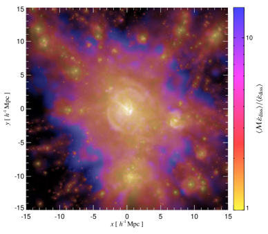
Supplementary Figure 14: Energy dissipation rate at shocks in a simulated galaxy cluster (non-cool core, $M=1.5\times 10^{15}\,\mathrm{M}_{\odot}$). Top: the Mach number of structure formation shocks weighted by the energy dissipation rate in colour (while the brightness displays the logarithm of the dissipation rate)[2007MNRAS.378..385P]. Note that most of the energy density is dissipated in weak shocks inside groups and clusters. Bottom: normalised energy density dissipation rate as a function of cluster-centric radius. The profile peaks in the centre and declines towards the periphery. On top of this average profile, there is a merging shock wave visible at $r=0.6\,R_{200}=1.4\,\mathrm{Mpc}$ as well as the accretion shock at $r=2\,R_{200}$; both of which have counterparts in the projected image at the top.

A very interesting piece of evidence arises from studies of the evolution of the temperature profile in cosmological cluster simulations that employ isotropic conduction at $1/3$ of the classical Spitzer value. They show that even hot clusters, that have very efficient heat conduction, are not able to establish an isothermal profile[2004MNRAS.351..423J, 2004ApJ...606L..97D]. This suggests that shocks driven by gravitational infall can act as a selective heating source. It is very instructive to consider the energy dissipation at structure formation shocks in cosmological simulations[2006MNRAS.367..113P, 2007MNRAS.378..385P]. Figure 14 shows a high-resolution hydrodynamic simulation of a galaxy cluster using the ‘zoomed initial conditions’ technique within a cosmological framework[2008MNRAS.385.1211P]. Using the distributed-memory parallel TreeSPH code GADGET-2, the simulations followed radiative cooling of the gas and star formation. They also identified the Mach numbers of cosmological formation shocks[2006MNRAS.367..113P] that dissipate gravitational energy in the process of hierarchical structure growth. The important point to take away is that most of the energy of these shocks is dissipated towards the cluster centres in weak flow shocks. This can be understood as the energy flux through the shock surface, $\dot{E}_{\mathrm{diss}}/R^{2}\sim\rho\upsilon^{3}$, that will be dissipated at these formation shocks, is maximised in the dense cluster cores. To order of magnitude, we expect the heating to take place on a dynamical time scale of $\tau_{\mathrm{dyn}}\simeq 1$ Gyr. This time scale is shorter or comparable to the thermal conduction time over significant cluster scales, $\tau_{\mathrm{cond}}=\lambda^{2}/\chi_{\mathrm{C}}\simeq 2.3\,\mathrm{Gyr}\,(\lambda/1\,\mathrm{Mpc})^{2}$, where $\chi_{\mathrm{C}}=8\times 10^{31}(T/10\,\mathrm{keV})^{5/2}(n/5\times 10^{-3}\,\mathrm{cm}^{-3})^{-1}\,\mathrm{cm}^{2}\,\mathrm{s}^{-1}$ is the Spitzer thermal diffusivity. Hence one would expect a stationary temperature profile that should always show a moderate temperature gradient which would be needed to power the MTI and keep the magnetic field lines preferentially radial.

Since the thermal conduction time scales with the square of the length scale in question, it will always win over the dynamical time or sound crossing time on small enough length scales and thermally stabilise these regions – provided we have a mechanism that ensures efficient conduction close to the Spitzer value. Clearly, we need detailed MHD simulations of cluster formation in a cosmological framework that include anisotropic conduction to confirm this picture. However, our result of a preferentially radial field orientation in Virgo strongly suggests that gravitational heating by accreted substructures seems to maintain the temperature gradients even in the presence of the MTI. This indirectly confirms a prediction of the hierarchical structure formation scenario in which a halo constantly undergoes mergers and accretes smaller mass objects that gravitationally heat the ICM through shock wave heating.

A note here is in order as completely randomly-oriented magnetic fields could also sustain effective conduction at $1/3$ of the Spitzer value. This however assumes that field line-wandering is in fact volume filling, i.e. a set of initially close-by field lines is not constrained to a two dimensional hyper surface. One could image idealised models that would not predict conduction at $1/3$ of Spitzer; one realisation of such a model for the growth of clusters that is able to explain the observed entropy profile in clusters is the model of smooth accretion[2005RMP...77...207V]. Suppose that mass accretes in a series of concentric shells that have negligible pressure and entropy and are initially comoving with the Hubble flow. Once these shells decelerate and reach zero velocity at the turnaround radius, they fall back under the influence of gravity of the previously collapsed shells and encounter the accretion shock at about the virial radius. There will be a higher entropy generated for later accreting shells leading to an overall stable entropy profile[2005RMP...77...207V]. Presumably each of these shells carries their flux-frozen magnetic field that in this simple picture does not intersect with the field in the other shells. Once established, the stably stratified entropy profile suppresses convective motions and prevents radial mixing (assuming for a moment that the MTI is suppressed by some mechanism). Of course within hierarchical structure formation, these idealised hyper surfaces will never be perfectly separated and there will be some degree of mixing. However, a small degree of mixing should still suppress efficient conduction and calls for an effect that actively builds up radial field components – one prime candidate would be the MTI.

10 The Virgo cluster

Supplementary Figure 15: Profiles of gas properties and the magnetic field of Virgo. Top, middle: profiles of the electron density (described by a double-beta model where we show both components with dotted lines) and entropy variable $K=kT_{\mathrm{x}}n_{\mathrm{e}}^{-2/3}$ of the Virgo cluster as inferred from X-ray data[2002A&A...386...77M]. Note the asymptotic behaviour of the entropy variable $K\propto r^{0.9}$ for large radii. Bottom: illustrative profile of a magnetic field model with a central field strength of $B_{0}=8\,\mu$G and an assumed scaling with the gas density of $B\propto n^{\alpha_{B}}$. We show plausible ranges for the scaling parameter as determined from cosmological cluster simulations[1999A&A...348..351D, 2001A&A...378..777D] and Faraday rotation measurements[2005A&A...434...67V] and note the choice $\alpha_{B}=0.7$ corresponds to the flux freezing condition.

In which category of clusters does the Virgo cluster fall into – is it a cooling core cluster (CC) or a non-cooling core (NCC)? It turns out that this question is not as simple to answer as one might think. Due to its proximity, already ROSAT and later on XMM-Newton resolved a small cooling core at radii $<14$ kpc[1994Natur.368..828B, 2002A&A...386...77M]. But how does its overall appearance compare to the clusters in the Chandra sample[2008ApJ...683L.107C], in particular if we placed it to higher redshifts?

First we note that there is a discrepancy in the literature about the virial mass and radius of the Virgo cluster. The X-ray community converged on a value for its virial mass of $M_{200}=2.1\times 10^{14}\,\mathrm{M}_{\odot}$ resulting in a virial radius of $R_{200}=0.95$ Mpc[1999A&A...343..420S]. We define the virial mass $M_{\Delta}$ and virial radius $R_{\Delta}$ as the mass and radius of a sphere enclosing a mean density that is $\Delta=200$ times the critical density of the Universe, $\rho_{\mathrm{crit}}=3H_{0}^{2}/(8\pi G)$. The corresponding virial temperature of the halo is

$$kT_{200}=\frac{G\,M_{200}\,\mu\,m_{\mathrm{p}}}{2\,R_{200}}\simeq 2.8\mbox{ keV},$$ (33)

where $\mu\simeq 0.6$ denotes the mean molecular weight. This corresponds well with the deprojected temperature profiles from X-ray observations[1994Natur.368..828B, 2002A&A...386...77M] that observed a maximum temperature of $\simeq 3$ keV at a radius of 200 kpc (corresponding to 40 arcmin). Conversely, applying a relativistic Tolman-Bondi model of the Virgo cluster to a sample of 183 galaxies with measured distances within a radius of 8 degrees from M87, Virgo’s virial mass is found to be $M_{200}=7\times 10^{14}\,\mathrm{M}_{\odot}$[2001A&A...375..770F]. A similar large mass estimate of $M_{200}=1.3\times 10^{15}\,\mathrm{M}_{\odot}$ is supported by modelling of the velocity field of the local super-cluster, assuming a mass-to-light ratio of $150~{}\mathrm{M}_{\odot}/\mathrm{L}_{\odot}$ in the field, but 1000 for the Virgo cluster[1999elss.conf..296T]. For the purpose of this section we use however the virial estimates from the X-ray measurements.

We use the deprojected density profile[2002A&A...386...77M] (described by a double-beta model) as well as a fit to the temperature profile[2004A&A...413...17P] in order to construct the entropy profile. To this end, we use the X-ray entropy variable[1999Natur.397..135P] $K=kT_{\mathrm{x}}n_{\mathrm{e}}^{-2/3}$ that is derived from the equation for the adiabatic index, $K\propto P\rho^{-5/3}$. For radii $r<2$ kpc we observe an entropy core, outside a power-law behaviour that asymptotes $K\propto r^{0.9}$. This is somewhat shallower compared to that of most clusters of the Chandra sample[2008ApJ...683L.107C], $K\propto r^{1.1-1.2}$. This discrepancy will be reinforced when adopting a declining temperature profile in the outskirts; a behaviour possibly caused by the low X-ray counts in these regions due to the large angular extent of seven degrees on the sky.

We now determine the entropy core value of Virgo if we placed it successively at higher redshifts, i.e. we address angular resolution effects. From $K\propto r^{0.9}$ outside $r=2$ kpc, we conclude any weighting (over volume or emission) will produce the same radial behaviour, i.e. the inferred value for the central entropy $\tilde{K}_{0}$ is always dominated by the value of the entropy profile at the radius corresponding to the angular resolution $\theta$ of an X-ray instrument or the binning algorithm used for the analysis[2008ApJ...683L.107C]. The physical radius $r(z)=D_{\mathrm{ang}}(z)\tan\theta$, corresponding to $\theta=5^{\prime\prime}$ increases as a function of redshift with the angular diameter distance $D_{\mathrm{ang}}$; and so does $\tilde{K}_{0}$. Adopting the entropy profile of Fig. 15, we solve the equation $\tilde{K}[r(z)]>30\,\mbox{keV cm}^{2}$ for $z$. We find that Virgo – placed at a redshift $z>0.13$ – would show a high-entropy core in agreement with NCCs. The very low H$\alpha$ luminosity[1999MNRAS.306..857C] $L_{\mathrm{H}\alpha}\simeq 10^{39}\,\mathrm{erg/s}$, being below most of the upper limits in the Chandra sample[2008ApJ...683L.107C], confirms this picture that Virgo might be on its transition to a cool core at the centre but still shows all signs of a NCC on large scales.