Neutron electric polarizability

Abstract:

We use the background field method to extract the “connected” piece of the neutron electric polarizability. We present results for quenched simulations using both clover and Wilson fermions and discuss our experience in extracting the mass shifts and the challenges we encountered when we lowered the quark mass. For the neutron we find that as the pion mass is lowered below $500\mathop{\hbox{MeV}}$, the polarizability starts rising in agreement with predictions from chiral perturbation theory. For our lowest pion mass, $m_{\pi}=320\mathop{\hbox{MeV}}$, we find that $\alpha_{n}=3.8(1.3)\times 10^{-4}\mathop{\hbox{fm}}^{3}$, which is still only one third of the experimental value. We also present results for the neutral pion; we find that its polarizability turns negative for pion masses smaller than $500\mathop{\hbox{MeV}}$ which is puzzling.

1 Introduction

Hadron polarizabilities measure the ability of the electromagnetic field to deform the hadrons. At the lowest order, the effect of the electromagnetic field on the hadrons is parametrized by the effective Hamiltonian:

$$H_{em}=-\vec{p}\cdot\vec{E}-\vec{\mu}\cdot\vec{B}-\frac{1}{2}(\alpha E^{2}+\beta E^{2})+\ldots,$$ (1)

where $\vec{p}$ and $\vec{\mu}$ are the electric and magnetic dipole moments and $\alpha$ and $\beta$ are the electric and magnetic polarizabilities. Due to the time reversal symmetry of the strong forces, the electric dipole moment of the hadrons is zero and the electric field effects are quadratic in the strength of the electric field. The electric polarizability, $\alpha$, measures the induced electric dipole and it is the most important parameter needed to describe the interaction of weak electric fields with the hadrons.

Experimentally, the electric polarizability is measured in Compton scattering off nuclear targets – the experiments allow access only to a combination of electric and magnetic polarizabilities and further modeling is required to disentangle these parameters. Extracting the polarizabilities for the neutron is especially difficult since there are no free neutron targets; the best experimental numbers come from neutron scattering off lead [1] and deuteron [2]. The experimentally determined value for the electric polarizability is $\alpha_{n}=12.5(2.5)\times 10^{-4}\mathop{\hbox{fm}}^{3}$.

Lattice QCD calculations of electromagnetic polarizabilities have a long history: the first study was published 20 years ago [3]. This study employed the background field method and used quenched staggered fermions and rather heavy quark masses; however, the results looked promising. Further studies employing quenched wilson and clover fermions found again good agreement with the experimental value [4]. Recently, the interest in the problem was renewed. A number of groups are trying to determine the polarizability in the chiral limit [5, 6, 7, 8] and new issues have surfaced. Some problems with the method used to introduced the background field were resolved [8, 9] and the new studies produce much smaller values for the neutron polarizability. The new values are no longer in good agreement with the experimental value as we can see from Fig. 1; however, chiral perturbation theory predicts that the electric polarizability diverges in the chiral limit and it is possible that the disagreement is only due to the relatively heavy quark masses used in the current lattice QCD simulations.

Our ultimate goal is to compute the electric polarizability of the neutron and other hadrons in the physical limit and to compare the lattice predictions with the experimental results. The purpose of the current study is to determine the methodology to compute electric polarizability; in particular we focus on the fitting methods used to extract the electric mass shifts and the range of quark masses needed to be able to perform the chiral extrapolation. To clarify this last point: since simulations using the physical quark masses are not yet feasible, chiral extrapolations will need to be used. We have to determine how small the quark masses need to be to observe the chiral behavior. From our previous study [8], we know the neutron polarizability is rather flat for pion masses larger than $500\mathop{\hbox{MeV}}$; in the current study we use a pion mass down to $320\mathop{\hbox{MeV}}$. Chiral perturbation theory predicts that the divergent behavior will also appear in quenched simulations [10] and since the purpose of the current study is exploratory in nature, we use quenched ensembles.

The plan of the paper is the following: we start by briefly reviewing the background field method; we then present the fitting method we used to extract the mass shifts and compare it with the method used in our previous study. We use the neutral pion as an example because the signal is cleanest in the pseudoscalar channel. We present our results for the neutron polarizability and conclude by discussing our plans for the future.

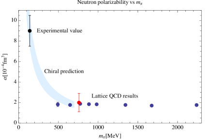
Figure 1: Neutron electric polarizability: the red and blue points are lattice QCD results [5, 8] and the black point is the experimental result [11]. The chiral prediction is a $1/m_{\pi}$ fit that is forced to go through the experimental value and asymptote to the lattice QCD values.

2 Background field method

In this section we describe the method we use to compute the electric polarizabilities: the background field method. The electromagnetic field is introduced via minimal coupling, i.e. the covariant derivative in the presence of the electromagnetic potential $A_{\mu}$ is

$$D_{\mu}=\partial_{\mu}-igG_{\mu}-iqA_{\mu},$$ (2)

where $G_{\mu}$ is the color field. On the lattice, this amounts to modifying the links:

$$U_{\mu}\rightarrow U_{\mu}e^{-iaqA_{\mu}}.$$ (3)

The polarizability is determined by measuring the change in the mass of a hadron when we turn the background field on. From Eq. 1 it can be inferred that the shift in the energy is negative for a positive electric polarizability. This is still true on the lattice if the electric field is introduced via a real factor [8, 9]. On the lattice it is convenient to work with imaginary factors; in this case the relationship between the energy shift and the polarizability needs to be adjusted. For example, if we introduce an electric field in the $x$ direction using $U_{x}\rightarrow U_{x}e^{-iaqEt}$ then

$$\Delta m=+\frac{1}{2}\alpha E^{2}.$$ (4)

The effect of the electric field on the hadron masses is very weak and the mass shifts we have to measure are minute. In fact, the mass shifts are usually much smaller than the stochastic error in the determination of the hadron masses. To extract such tiny shifts we rely on the correlation between the hadron propagators measured on the same color gauge background. Denote with $G_{0}(t)$ the hadron propagator of interest and with $G_{E}(t)$ the same propagator measured with the electric field turned on. The error of each of these propagators is larger than their difference, but they are strongly correlated. To measure the mass shift we look at their ratio which for large times is expected to be dominated by the lowest energy in the channel:

$$R(t)=\frac{G_{E}(t)}{G_{0}(t)}\xrightarrow{\mbox{\tiny$t\rightarrow\infty$}}\frac{A^{\prime}e^{-m^{\prime}t}}{Ae^{-mt}}\propto e^{-\Delta mt}.$$ (5)

We can define an “effective mass” based on this ratio, $a\Delta m_{\rm eff}\equiv-\ln R(t+1)/R(t)$, and see whether this quantity exhibits a plateau. In Fig. 2 we show such an effective mass plot for the neutral pion; for this heavy quark case, we get a very good plateau and we can use a single exponential fit in the range $t\in[20,40]$ to extract the mass shift. At lower quark masses the propagators become noisier and more sophisticated techniques are needed to extract the mass shift.

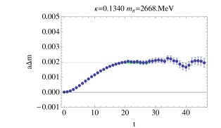
Figure 2: The effective mass shift for a heavy pion; this is based on the ratio defined in Eq. 5.

3 Extracting the mass shift

As we emphasized in the last section, the mass shift induced by the electric field is tiny and we need special methods to determine it. Ideally, we would be able to generate propagators that produced good plateaus for the effective mass shift. In our previous study [8] we used $24^{4}$ lattices with $a=0.093\mathop{\hbox{fm}}$. In Fig. 3 we present the effective mass plots for the mass shift of the neutron (note that the mass shift are negative because in that study we introduced the electric field using a real factor). We cannot detect any plateau in these figures – the reason for it is two fold: for heavier quark masses it looks like the lattice is too short to form a plateau and for lighter masses the signal gets noisy before we can detect a plateau.

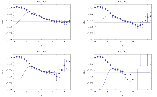
Figure 3: The effective mass shift for neutron on $24^{4}$ lattices; the solid line represents the results of the fit.

To solve this problem, we used a two exponential fit to extract the mass shift. Since we are fitting the ration of two propagators, the two exponential fit involves 6 independent parameters:

$$\frac{G_{E}(t)}{G_{0}(t)}\rightarrow\frac{W_{1}^{\prime}e^{-m_{1}^{\prime}t}+W_{2}^{\prime}e^{-m_{2}^{\prime}t}}{W_{1}e^{-m_{1}t}+W_{2}e^{-m_{2}t}}=\frac{A_{1}e^{-\delta m_{1}t}+A_{2}e^{-\delta m_{2}}}{1+A_{3}e^{-\delta m_{3}t}}.$$ (6)

Since 6 parameter fits were too unstable, we extracted $A_{3}$ and $\delta m_{3}$ from a two exponential fit for $G_{0}(t)$ and used these values as priors for the 6 parameter fit. The results of these fits are plotted with solid lines in Fig. 3.

For the new set of runs we used lattices of size $24^{3}\times 48$, so that we can observe the plateau, at least for heavy quark masses. We also used a different method to extract the mass shift. The main reason we decided to use a different method is that the double exponential method used above reuses the $G_{0}(t)$ data and this forces us to use time-consuming jackknife or bootstrap when estimating the errors. Moreover, the method proved cumbersome to use when we decided to scan the fitting range; these scans are needed to understand how robust the results are. The new method we used is faster and more stable – it allows us to scan the ranges efficiently and also it produces error estimates that are trustworthy. The method is simply based on a correlated fit that uses both $G_{0}(t)$ and $G_{E}(t)$ data simultaneously; the difference vector is defined to be:

$$\delta_{i} \equiv f(t_{i})-G_{0}(t_{i}),\quad\quad\quad{\rm for}\quad i=1,\dots,n$$

$$\delta_{i} \equiv \bar{f}(t_{i-n})-G_{E}(t_{i-n}),\quad{\rm for}\quad i=n+1,\dots,2n$$ (7)

where $f(t)=A\exp(-mt)$ and $\bar{f}(t)=A^{\prime}\exp(-(m+\Delta m)t)$ and $n$ is the number of time slices used in the fit. The fitting function then minimizes $\chi^{2}=\frac{1}{2}\delta^{T}C^{-1}\delta$, where $C$ is the $2n\times 2n$ correlation matrix. The two $n\times n$ diagonal blocks of this matrix are the usual correlation matrices for $G_{0}(t_{i})$ and $G_{E}(t_{i})$ and the off-diagonal blocks represent the cross-correlations (which are strong since these propagators are evaluated on the same configurations). The fit depends on 4 parameters and $\Delta m$ is the mass shift we want – this also allows us to get the error bars for the mass shift directly from the $\chi^{2}$ fitting analysis, a procedure that is both fast and with a solid theoretical foundation. In Fig. 4 we show the results of fitting the pion propagators using this method and compare it with the plateaus seen in the effective mass plot; the agreement is encouraging. This is the method that we employ to compute the mass shift for the results presented in this paper.

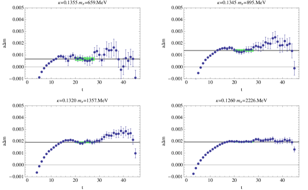
Figure 4: The effective mass shift for neutral pion compared with the result of the fit. The solid lines indicate the results of the fit and the green boxes’ height indicate the error estimate; the width of the green boxes is used to indicate the range of the fit. The fit agrees with the plateaus in the effective mass plots.

4 Simulation parameters

All our simulations are run on quenched ensembles, generated using Wilson gauge action with $\beta=6.0$; this corresponds to a lattice spacing of $a=0.093\mathop{\hbox{fm}}$. We had three sets of runs, and the relevant information is presented in Table 1.

Ensemble	fermion type	number of configurations	pion mass range ($\mathop{\hbox{MeV}}$)	exceptional
${\cal E}_{1}$	clover	1000	500 – 2200	34
${\cal E}_{2}$	Wilson	300	580 – 2700	0
${\cal E}_{3}$	Wilson	200	320 – 750	4

Table 1: The parameters for the three ensembles used in this study.

The boundary conditions are important for the background field method. It turns out that a constant field is not easy to introduce on a lattice with periodic boundary conditions without creating a discontinuity. In this study we use Dirichlet boundary conditions in both time direction and the direction of the electric field.

One problem that we had to deal with is the presence of exceptional configurations at the lower quark masses; the surprise was that we get exceptional configurations for pion masses as large as $500\mathop{\hbox{MeV}}$ for the ensemble ${\cal E}_{1}$. We detected the presence of exceptional configurations from the fact that the hadron propagators were a lot noisier on the entire ensemble than on a subset. The method we used to detect and filter these configurations out was the following: for every propagator of interest we looked at the smallest quark mass sector and for every time-slice we computed the mean and its standard deviation:

$$\bar{G}(t)=\frac{1}{N_{\rm conf}}\sum_{i}G^{(i)}(t),\quad\quad\sigma_{G(t)}=\sqrt{\frac{1}{N_{\rm conf}}\sum_{i}(G^{(i)}(t)-\bar{G}(t))^{2}}.$$ (8)

If the propagator for a configuration has at least one time-slice with $|G^{(i)}(t)-\bar{G}(t)|>10\sigma_{G(t)}$, we consider that configuration to be exceptional. For a normally distributed random variable this should happen extremely infrequently. The effect of this filtering is shown in Fig. 5: we see that the heavier quark mass propagators are unaffected while the small mass propagator is significantly improved.

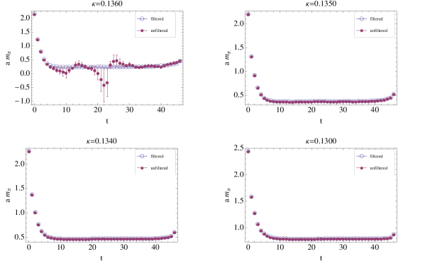
Figure 5: The pion propagator for a subset of quark masses from ensemble ${\cal E}_{1}$ – the emty symbols are the propagator after filtering out the exceptional configurations and the full symbols represent the original propagator.

The last topic we discuss is the electric field strength. In dimensionless units the value of the field is $\eta=a^{2}qE=0.00576$. In the macroscopic realm, this is a very strong field – on the other hand it is comparable with the electric field a quark feels when placed about $1\mathop{\hbox{fm}}$ away from another quark. Thus the shift induced by this field should be comparable with the electromagnetic mass shift in hadrons which is known to be small. Even better, we can determine whether the electric field is small enough by checking the scaling of the mass shift with the increase of the electric field. We have not run the simulations with different electric field, since we have already seen in our previous studies that this field is small enough [4, 8]. However, it is actually possible to check using the data that we have whether the scaling is obeyed; since the up and down quark have the same mass in the isosipin limit but different charges we can ask whether the mass shift for the $\bar{u}\gamma_{5}u$ and $\bar{d}\gamma_{5}d$ propagators scales appropriately. In Fig. 6 we plot the effective mass shift for these two propagators; we scale the $\bar{d}\gamma_{5}d$ propagator by a factor of $4$ (in the weak field limit the mass shift is proportional to the square of the charges). It is easy to see that the agreement is almost perfect for all quark masses; since the agreement is so good for the effective mass shift, any mass shift extracted from these propagators will scale perfectly. We conclude that the field we used in our simulation is weak enough.

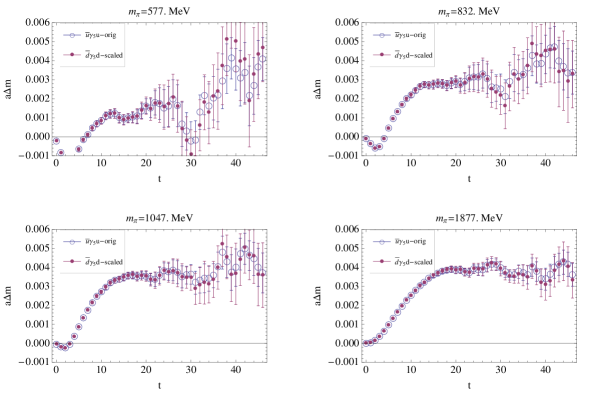
Figure 6: The effective mass shift for $\bar{u}\gamma_{5}u$, empty symbols, and scaled $\bar{d}\gamma_{5}d$, full symbols.

5 Simulation results

In this section we present our results for the neutral pion and the neutron. The results presented here do not include the dynamical effects: the quarks are treated in the quenched approximation and also, the sea quarks are not charged. We expect that these effects do not play a very important role for the masses we are simulating, but they will be important in the chiral limit.

In Fig. 7 we show our results for the neutral pion. We want to stress that the results we present for the neutral pion do not include the disconnected piece; in the isospin limit this piece should be zero. However, the presence of the electric field breaks the isospin symmetry even when the masses of the up and down quarks are zero. As such, the results we present for the pion are only an approximation. We fitted the propagators in the time window $t\in[15,33]$. The first thing to notice is that the clover and Wilson discretizations produce similar results: in the range $m_{\pi}\in[500\mathop{\hbox{MeV}},800\mathop{\hbox{MeV}}]$ they agree within error bars. This seems to indicate that the discretization errors are small and that we have a fine enough lattice spacing. For large quark masses, while qualitatively similar, the values differ more.

It is interesting to note that for low pion masses, the polarizability seems to decrease. In fact, around $m_{\pi}=500\mathop{\hbox{MeV}}$ the polarizability turns negative and it seems to diverge. This is in agreement with the results produced in dynamical simulations using clover fermions [6, 7]. We note that our values agree well with the dynamical simulations, indicating that the dynamical effects are still small at the pion masses we are studying. It should be noted that while the value for the pion polarizability is expected to be negative, this is a result of the disconnected piece that we have not included in our calculation. The expectation is that, for the propagator we compute, the polarizability should be positive [7]. The most likely culprit seems to be the finite volume effects, that are expected to be large for polarizability – we plan to investigate this issue further.

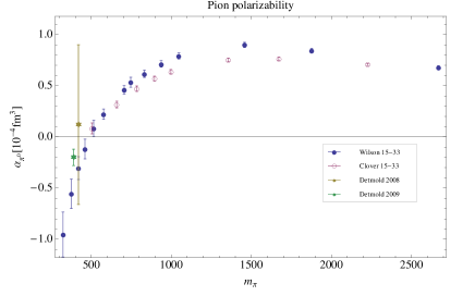
Figure 7: Pion polarizability: the blue points are our result with Wilson fermions, the empty point are the clover results and the stars are the results from [6, 7].

In Fig. 8 we plot our results for the electric polarizability of the neutron. Once again, we see that the Wilson and clover results agree nicely. The results also agree well with those produced by dynamical simulations – this again shows that the dynamical effects are relatively small at these pion masses. Finally, the most important feature is that for pion masses smaller than $500\mathop{\hbox{MeV}}$ the polarizability seems to increase rapidly. We are finally seeing the predicted increase in the polarizability as we approach the chiral limit. Moreover, looking at the right panel in Fig. 8, it is conceivable that if the trend continues we will reproduce the experimental result when we reach the physical limit. However, our result is still only about $3.8(1.3)\times 10^{-4}\mathop{\hbox{fm}}^{3}$ for $m_{\pi}=320\mathop{\hbox{MeV}}$, about a third of the experimental value – there is still quite a bit to go to reach the physical limit.

To sum up, we find that the clover and Wilson fermions produce similar results for both the pion and the neutron; this tells us that the discretization errors should be smaller than our current error bars. Our results are in good agreement with polarizabilities measured on dynamical ensembles which indicates that the dynamical effects are not very large. The pion polarizability seems to be more and more negative as we lower the quark mass, a result that is puzzling. The neutron polarizability shoots up when the pion mass is lowered below $500\mathop{\hbox{MeV}}$ – this gives us hope that we can use chiral perturbation theory to extrapolate to the physical point.

6 Outlook

The most important conclusion of our study is that the behavior predicted by chiral perturbation theory for the neutron polarizability seems to appear for pion masses in the range $300\mathop{\hbox{MeV}}$ to $500\mathop{\hbox{MeV}}$. The error bars in the current study are too large to allow us to extrapolate the result, but this is mainly due to our rather small statistics for ensemble ${\cal E}_{3}$. We are currently collecting more statistics and we plan to fit the data and extrapolate it to the physical point. We also plan to run simulations at even lower quark masses to improve the quality of our extrapolation. The exceptional configurations might be a problem – in that case we plan to use a better discretization for the fermions. As a cheap alternative, we can use nHYP fermions or, if we have to, overlap fermions since they don’t suffer from this issue.

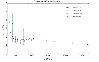
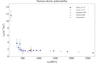
Figure 8: Neutron polarizability: the blue points are our result with Wilson fermions, the empty point are the clover results and the stars are the results from [6, 5] and the experimental result. The left panel doesn’t show the experimental point to allow a better view of the lattice results.

The study produced also a puzzle regarding the polarizability of the neutral pion. As it was pointed out [7], the most likely culprit is the finite volume effects. In our case the finite volume effects are mainly due to our choice of boundary conditions. We plan to investigate the interplay between the boundary conditions and the finite volume effects on the polarizability.

In the long run, we plan to include the dynamical effects of the sea quarks on the polarizability. At this point, we feel that the best use for our computational resources is to pin down as best as we can the method to determine the polarizability in the context of quenched approximation and to determine its value at the physical point. The strategy that we plan to use to charge the sea quarks is reweighting and we expect that this would be very resource intensive. To complete the calculation, we need to also use dynamically generated configurations; while this is an important step to finalize the calculation, we feel that its contribution is the smallest while the computational resources needed are significant. As such, this will be the last step in our program.

References

- [1] J. Schmiedmayer, P. Riehs, J. A. Harvey and N. W. Hill, Phys. Rev. Lett. 66, 1015 (1991).
- [2] K. Kossert et al., Eur. Phys. J. A 16, 259 (2003) [arXiv:nucl-ex/0210020].
- [3] H. R. Fiebig, W. Wilcox and R. M. Woloshyn, Nucl. Phys. B 324, 47 (1989).
- [4] J. C. Christensen, W. Wilcox, F. X. Lee and L. m. Zhou, Phys. Rev. D 72, 034503 (2005) [arXiv:hep-lat/0408024].
- [5] M. Engelhardt [LHPC Collaboration], Phys. Rev. D 76, 114502 (2007) [arXiv:0706.3919 [hep-lat]].
- [6] W. Detmold, B. C. Tiburzi and A. Walker-Loud, arXiv:0809.0721 [hep-lat].
- [7] W. Detmold, B. C. Tiburzi and A. Walker-Loud, Phys. Rev. D 79, 094505 (2009) [arXiv:0904.1586 [hep-lat]].
- [8] A. Alexandru and F. X. Lee, arXiv:0810.2833 [hep-lat].
- [9] E. Shintani et al., Phys. Rev. D 75, 034507 (2007) [arXiv:hep-lat/0611032].
- [10] W. Detmold, B. C. Tiburzi and A. Walker-Loud, Phys. Rev. D 73, 114505 (2006) [arXiv:hep-lat/0603026].
- [11] S. R. Beane, M. Malheiro, J. A. McGovern, D. R. Phillips and U. van Kolck, Nucl. Phys. A 747, 311 (2005) [arXiv:nucl-th/0403088].