Local Statistical Modeling via Cluster-Weighted Approach with Elliptical Distributions

Abstract

Cluster Weighted Modeling (CWM) is a mixture approach regarding the modelisation of the joint probability of data coming from a heterogeneous population. Under Gaussian assumptions, we investigate statistical properties of CWM from both the theoretical and numerical point of view; in particular, we show that CWM includes as special cases mixtures of distributions and mixtures of regressions. Further, we introduce CWM based on Student-t distributions providing more robust fitting for groups of observations with longer than normal tails or atypical observations. Theoretical results are illustrated using some empirical studies, considering both real and simulated data.

1 Introduction

Finite mixture models provide a flexible approach to statistical modeling of a wide variety of random phenomena characterized by unobserved heterogeneity. In those models, dating back to the work of Newcomb (1886) and Pearson (1894), it is assumed that the observations in a sample arise from unobserved groups in the population and the purpose is to identify the groups and estimate the parameters of the conditional-group density functions. If there are no exogenous variables explaining the means and the variances of each component, we refer to unconditional mixture models, i.e. the so-called Finite Mixtures of Distributions (FMD), developed for both normal and non-normal components, see e.g. Everitt and Hand (1981); Titterington et al. (1985); McLachlan and Basford (1988); McLachlan and Peel (2000); Frühwirth-Schnatter (2005). Otherwise, we refer to conditional mixture models, i.e. Finite Mixtures of Regression models (FMR) and Finite Mixture of Generalized Linear Models (FMGLM), see e.g. DeSarbo and Cron (1988); Jansen (1993); Wedel and De Sarbo (1995); McLachlan and Peel (2000); Frühwirth-Schnatter (2005). These models are also known as mixture-of-experts models in machine learning (Jordan and Jacobs, 1994; Peng et al., 1996; Ng and McLachlan, 2007, 2008), switching regression models in econometrics (Quand, 1972), latent class regression models in marketing (De Sarbo and Cron, 1988; Wedel and Kamakura, 2000), mixed models in biology (Wang et al., 1996). An extension of FMR are the so-called Finite Mixtures of Regression models with Concomitant variables (FMRC) (Dayton and Macready, 1988; Wedel, 2002), where the weights of the mixture functionally depend on a set of concomitant variables, which may be different from the explanatory variables and are usually modeled by a multinomial logistic distribution.

The present paper focuses on a different mixture approach, which regards the modelisation of the joint probability of a response variable and a set of explanatory variables. In the original formulation, proposed by Gershenfeld (1997), it was called Cluster-Weighted Modeling (CWM) and was developed in the context of media technology, in order to build a digital violin with traditional inputs and realistic sound (Gershenfeld et al., 1999; Schöner, 2000; Schöner and Gershenfeld, 2001). Wedel (2002) refers to such model as the saturated mixture regression model. Moreover, Wedel and De Sarbo (2002) propose an extensive testing of nested models for market segment derivation and profiling. In the literature, CWM has been developed essentially under Gaussian assumptions; here we set such models in a quite wide framework by considering both direct and indirect applications.

In this paper we reformulate CWM from a statistical point of view and first, we prove that, under suitable assumptions, FMD, FMR and FMRC are special cases of CWM. Secondly, we introduce CWM based on Student-t distributions, which have been proposed in the literature in order to provide more robust fitting for groups of observations with longer than normal tails or atypical observations (Lange et al., 1989; Bernardo and Girón, 1992; McLachlan and Peel, 2000; Peel and McLachlan, 2000; Nadarajah and Kotz, 2005). Theoretical results will be illustrated using some numerical studies based on both real and simulated data.

The rest of the paper is organized as follows. In Section 2 CWM is introduced in a statistical framework; this formulation enables, in Section 3, a comparison with FMD, FMR and FMRC under Gaussian assumptions; in Section 4 Student-$t$ CWM is introduced and the links with Finite Mixtures of Student-t distributions (FMT) are discussed; then, some empirical studies based on both real and simulated datasets are discussed in Section 5. Finally, in Section 6 we provide some conclusions and remarks for further research. In the Appendix a geometrical analysis of the decision surfaces of CWM is reported.

2 Cluster-Weighted Modeling

In the original formulation, Cluster-Weighted Modeling (CWM) was introduced under Gaussian and linear assumptions (Gershenfeld, 1997); here we present CWM in a quite general setting. Let $(\mathbf{X},Y)$ be a pair of a random vector $\mathbf{X}$ and a random variable $Y$ defined on $\Omega$ with joint probability distribution $p(\mathbf{x},y)$, where $\mathbf{X}$ is the $d$-dimensional input vector with values in some space $\mathcal{X}\subseteq\mathbb{R}^{d}$ and $Y$ is a response variable having values in $\mathcal{Y}\subseteq\mathbb{R}$. Thus $(\mathbf{x},y)\in\mathcal{X}\times\mathcal{Y}\subseteq\mathbb{R}^{d+1}$. Suppose that $\Omega$ can be partitioned into $G$ disjoint groups, say $\Omega_{1},\ldots,\Omega_{G}$, that is $\Omega=\Omega_{1}\cup\cdots\cup\Omega_{G}$. CWM decomposes the joint probability $p(\mathbf{x},y)$ as follows:

$$p(\mathbf{x},y;\mbox{\boldmath$\theta$})=\sum^{G}_{g=1}p(y|\mathbf{x},\Omega_{g})\,p(\mathbf{x}|\Omega_{g})\,\pi_{g},$$ (1)

where $p(y|\mathbf{x},\Omega_{g})$ is the conditional density of the response variable $Y$ given the predictor vector $\mathbf{x}$ and $\Omega_{g}$, $p(\mathbf{x}|\Omega_{g})$ is the probability density of $\mathbf{x}$ given $\Omega_{g}$, $\pi_{g}=p(\Omega_{g})$ is the mixing weight of $\Omega_{g}$, ($\pi_{g}>0$ and $\sum^{G}_{g=1}\pi_{g}=1$), $g=1,\ldots,G$. Vector $\theta$ denotes the set of all parameters of the model. Hence, the joint density of $(\mathbf{X},Y)$ can be viewed as a mixture of local models $p(y|\mathbf{x},\Omega_{g})$ weighted (in a broader sense) on both the local densities $p(\mathbf{x}|\Omega_{g})$ and the mixing weights $\pi_{g}$.

Generalizing some ideas given in Titterington et al. (1985), pag. 2, we can distinguish three types of application of (1):

1. Direct application of type A. We assume that each group $\Omega_{g}$ is characterized by an input-output relation which can be written as $Y|\mathbf{x}=\mu(\mathbf{x};\mbox{\boldmath$\beta$}_{g})+\varepsilon_{g}$, where $\varepsilon_{g}$ is a random variable with zero mean and finite variance $\sigma^{2}_{g}$, and $\mbox{\boldmath$\beta$}_{g}$ denotes the set of parameters of $\mu(\cdot)$ function, $g=1,\ldots,G$.

2. Direct application of type B. We assume that there is a random vector $\mathbf{Z}$ defined on $\Omega=\Omega_{1}\cup\cdots\cup\Omega_{G}$ with values in $\mathbb{R}^{d+1}$ and each $\mathbf{z}\in\mathcal{Z}\subseteq\mathbb{R}^{d+1}$ belongs to one of these groups. Further, vector $\mathbf{z}$ is partitioned as $\mathbf{z}=(\mathbf{x}^{\prime},y)^{\prime}$ and we assume that within each group we write $p(\mathbf{z};\Omega_{g})=p((\mathbf{x}^{\prime},y)^{\prime};\Omega_{g})=p(y|\mathbf{x},\Omega_{g})\,p(\mathbf{x}|\Omega_{g})$. In other words, (1) is another form of density of FMD given by:

   $$p(\mathbf{z};\mbox{\boldmath$\theta$})=\sum^{G}_{g=1}p(\mathbf{z}|\Omega_{g})\pi_{g}=\sum^{G}_{g=1}p(y|\mathbf{x},\Omega_{g})\,p(\mathbf{x}|\Omega_{g})\,\pi_{g}.$$ (2)

3. Indirect application. In this case, the density function of CWM (1) is simply used as a mathematical tool for density estimation.

Throughout this paper we concentrate on direct applications. In this case, the posterior probability $p(\Omega_{g}|\mathbf{x},y)$ of unit $(\mathbf{x},y)$ belonging to the $g$-th group $(g=1,...,G)$ is given by:

$$p(\Omega_{g}|\mathbf{x},y)=\frac{p(\mathbf{x},y,\Omega_{g})}{p(\mathbf{x},y)}=\frac{p(y|\mathbf{x},\Omega_{g})p(\mathbf{x}|\Omega_{g})\pi_{g}}{\sum^{G}_{j=1}p(y|\mathbf{x},\Omega_{j})p(\mathbf{x}|\Omega_{j})\pi_{j}},\qquad g=1,\ldots,G$$ (3)

that is the classification of each unit depends on both marginal and conditional densities. Since $p(\mathbf{x}|\Omega_{g})\pi_{g}=p(\Omega_{g}|\mathbf{x})p(\mathbf{x})$, from (3) we get:

$$p(\Omega_{g}|\mathbf{x},y) =\frac{p(y|\mathbf{x},\Omega_{g})p(\Omega_{g}|\mathbf{x})p(\mathbf{x})}{\sum^{G}_{j=1}p(y|\mathbf{x},\Omega_{j})p(\Omega_{j}|\mathbf{x})p(\mathbf{x})}=\frac{p(y|\mathbf{x},\Omega_{g})p(\Omega_{g}|\mathbf{x})}{\sum^{G}_{j=1}p(y|\mathbf{x},\Omega_{j})p(\Omega_{j}|\mathbf{x})}\>,$$ (4)

with

$$p(\Omega_{g}|\mathbf{x})=\frac{p(\mathbf{x}|\Omega_{g})\pi_{g}}{\sum_{j=1}^{G}p(\mathbf{x}|\Omega_{j})\pi_{j}}=\frac{p(\mathbf{x}|\Omega_{g})\pi_{g}}{p(\mathbf{x})}\>,$$

where we set $p(\mathbf{x})=\sum_{j=1}^{G}p(\mathbf{x}|\Omega_{j})\pi_{j}$.

2.1 The basic model: linear Gaussian CWM

In the traditional framework, both marginal densities and conditional densities are assumed to be Gaussian, with $\mathbf{X}|\Omega\sim N_{d}(\mbox{\boldmath$\mu$}_{g},\mbox{\boldmath$\Sigma$}_{g})$ and $Y|\mathbf{x},\Omega_{g}\sim N(\mu(\mathbf{x},\mbox{\boldmath$\beta$}_{g}),\sigma^{2}_{\varepsilon,g})$, so that we shall write $p(\mathbf{x}|\Omega_{g})=\phi_{d}(\mathbf{x};\mbox{\boldmath$\mu$}_{g},\mbox{\boldmath$\Sigma$}_{g})$ and $p(y|\mathbf{x},\Omega_{g})=\phi(y;\mu(\mathbf{x};\mbox{\boldmath$\beta$}_{g}),\sigma^{2}_{\varepsilon,g})$, $g=1,\ldots,G$, where the conditional densities are based on linear mappings, so that $\mu(\mathbf{x};\mbox{\boldmath$\beta$}_{g})=\mathbf{b}^{\prime}_{g}\mathbf{x}+b_{g0}$, for some $\mbox{\boldmath$\beta$}=(\mathbf{b}_{g}^{\prime},b_{g0})^{\prime}$, with $\mathbf{b}\in\mathbb{R}^{d}$ and $b_{g0}\in\mathbb{R}$ . Thus, we get:

$$p(\mathbf{x},y;\mbox{\boldmath$\theta$})=\sum^{G}_{g=1}\phi(y;\mathbf{b}_{g}^{\prime}\mathbf{x}+b_{g0},\sigma^{2}_{\varepsilon,g})\,\phi_{d}(\mathbf{x};\mbox{\boldmath$\mu$}_{g},\mbox{\boldmath$\Sigma$}_{g})\,\pi_{g}\>,$$ (5)

with $\phi(\cdot)$ denoting the probability density of Gaussian distributions. Model (5) will be referred to as linear Gaussian CWM. In particular, the posterior probability (3) specializes as:

$$p(\Omega_{g}|\mathbf{x},y)=\frac{\phi(y;\mathbf{b}_{g}^{\prime}\mathbf{x}+b_{g0},\sigma^{2}_{\varepsilon,g})\phi_{d}(\mathbf{x};\mbox{\boldmath$\mu$}_{g},\mbox{\boldmath$\Sigma$}_{g})\pi_{g}}{\sum^{G}_{j=1}\phi(y;\mathbf{b}_{j}^{\prime}\mathbf{x}+b_{j0},\sigma^{2}_{\varepsilon,j})\phi_{d}(\mathbf{x};\mbox{\boldmath$\mu$}_{j},\mbox{\boldmath$\Sigma$}_{j})\pi_{j}}\qquad g=1,\ldots,G\>.$$ (6)

3 Linear Gaussian CWM and relationships with traditional mixture models

In this section we investigate some relationships between linear Gaussian CWM and some Gaussian-based mixture models. We shall prove that, under suitable assumptions, linear Gaussian CWM in (5) leads to the same posterior probability of such mixture models. In this sense, we shall say that CWM contains Finite Mixtures of Gaussians (FMG), Finite Mixtures of Regression models (FMR) and Finite Mixtures of Regression models with Concomitant variables (FMRC).

3.1 Finite Mixtures of Distributions

Let $\mathbf{Z}$ be a random vector defined on $\Omega=\Omega_{1}\cup\cdots\cup\Omega_{G}$ with joint probability distribution $p(\mathbf{z})$, where $\mathbf{Z}$ assumes values in some space $\mathcal{Z}\subseteq\mathbb{R}^{d+1}$. Assume that density $p(\mathbf{z})$ of $\mathbf{Z}$ has the form of a Finite Mixture of Distribution, i.e. $p(\mathbf{z})=\sum^{G}_{g=1}p(\mathbf{z}|\Omega_{g})\pi_{g}$ where $p(\mathbf{z}|\Omega_{g})$ is the probability density of $\mathbf{Z}|\Omega_{g}$ and $\pi_{g}=p(\Omega_{g})$ is the mixing weight of group $\Omega_{g}$, $g=1,\ldots,G$, see e.g. McLachlan and Peel (2000). Finally, denote with $\mbox{\boldmath$\mu$}_{g}^{(\mathbf{z})}$ and $\mbox{\boldmath$\Sigma$}_{g}^{(\mathbf{z})}$ the mean vector and the covariance matrix of $\mathbf{Z}|\Omega_{g}$ respectively.

Now let us set $\mathbf{Z}=(\mathbf{X}^{\prime},Y)^{\prime}$, where $\mathbf{X}$ is a random vector with values in $\mathbb{R}^{d}$ and $Y$ is a random variable. Thus, we can write

$$\mbox{\boldmath$\mu$}_{g}^{(\mathbf{z})}=\begin{pmatrix}\mbox{\boldmath$\mu$}_{g}^{(\mathbf{x})}\\ \mu_{g}^{(y)}\end{pmatrix}\quad{\rm and}\quad\mbox{\boldmath$\Sigma$}_{g}^{(\mathbf{z})}=\begin{pmatrix}\mbox{\boldmath$\Sigma$}^{(\mathbf{x}\mathbf{x})}_{g}&\mbox{\boldmath$\Sigma$}^{(\mathbf{x}\,y)}_{g}\\ \mbox{\boldmath$\Sigma$}^{(y\,\mathbf{x})}_{g}&\sigma^{2(y)}_{g}\end{pmatrix}\>.$$ (7)

Further, the posterior probability is given by:

$$p(\Omega_{g}|\mathbf{z})=\frac{p(\mathbf{z}|\Omega_{g})\pi_{g}}{\sum^{G}_{g=1}p(\mathbf{z}|\Omega_{g})\pi_{g}}\qquad g=1,\ldots,G\>.$$ (8)

We have the following result:

Proposition 1

Let $\mathbf{Z}$ be a random vector defined on $\Omega=\Omega_{1}\cup\cdots\Omega_{G}$ with values in $\mathbb{R}^{d+1}$, and assume that $\mathbf{Z}|\Omega_{g}\sim N_{d+1}(\mbox{\boldmath$\mu$}_{g},\mbox{\boldmath$\Sigma$}_{g})$ ($g=1,\ldots,G$). In particular, the density $p(\mathbf{z})$ of $\mathbf{Z}$ is a Finite Mixture of Gaussians (FMG):

$$p(\mathbf{z})=\sum^{G}_{g=1}\phi_{d+1}(\mathbf{z};\mbox{\boldmath$\mu$}_{g},\mbox{\boldmath$\Sigma$}_{g})\pi_{g}\>.$$ (9)

Then, $p(\mathbf{z})$ can be written like (5), that is as a linear Gaussian CWM.

Proof. Let us set $\mathbf{Z}=(\mathbf{X}^{\prime},Y)^{\prime}$, where $\mathbf{X}$ is a $d$-dimensional random vector and $Y$ is a random variable. According to well known results of multivariate statistics, see e.g. Mardia et al. (1979), from (9) we get

$$p(\mathbf{z}) =\sum^{G}_{g=1}\phi_{d+1}(\mathbf{z};\mbox{\boldmath$\mu$}_{g},\mbox{\boldmath$\Sigma$}_{g})\pi_{g}=\sum^{G}_{g=1}\phi_{d+1}((\mathbf{x},y);\mbox{\boldmath$\mu$}_{g},\mbox{\boldmath$\Sigma$}_{g})\pi_{g}$$

$$=\sum^{G}_{g=1}\phi_{d}(\mathbf{x};\mbox{\boldmath$\mu$}_{g}^{(\mathbf{x})}),\mbox{\boldmath$\Sigma$}_{g}^{(\mathbf{x}\mathbf{x})})\phi(y;\mu_{g}^{(y|\mathbf{x})},\sigma_{g}^{2(y|\mathbf{x})})\pi_{g}\>.$$

where $\mu_{g}^{(y|\mathbf{x})}=\mu_{g}^{(y)}+\mbox{\boldmath$\Sigma$}_{g}^{(y\mathbf{x})}\mbox{\boldmath$\Sigma$}_{g}^{(\mathbf{x}\mathbf{x})^{-1}}(\mathbf{x}-\mbox{\boldmath$\mu$}_{g}^{(\mathbf{x})})$ and $\sigma_{g}^{2(y|\mathbf{x})}=\mbox{\boldmath$\Sigma$}_{g}^{(yy)}$. If we set $\mathbf{b}_{g}=\mbox{\boldmath$\Sigma$}_{g}^{(y\mathbf{x})}\mbox{\boldmath$\Sigma$}_{g}^{(\mathbf{x}\mathbf{x})^{-1}}$, $b_{g0}=\mu_{g}^{(y)}-\mbox{\boldmath$\Sigma$}_{g}^{(y\mathbf{x})}\mbox{\boldmath$\Sigma$}_{g}^{(\mathbf{x}\mathbf{x})^{-1}}\mbox{\boldmath$\mu$}_{g}^{(\mathbf{x})}$ and $\sigma^{2}_{\varepsilon,g}=\sigma_{g}^{2(y|\mathbf{x})}$, then (9) can be written in the form (5). ∎

Using similar arguments, it can be shown that FMG and linear Gaussian CWM lead to the same distribution of posterior probabilities and thus CWM contains FMG.

We remark that the equivalence between FMG and CWM holds only for linear mappings $\mu(\mathbf{x};\mbox{\boldmath$\beta$}_{g})=\mathbf{b}^{\prime}_{g}\mathbf{x}+b_{g0}$ ($g=1,\ldots,G$), while, generally, Gaussian CWM

$$p(\mathbf{x},y;\mbox{\boldmath$\theta$})=\sum^{G}_{g=1}\phi(y;\mu(\mathbf{x};\mbox{\boldmath$\beta$}_{g}),\sigma^{2}_{\varepsilon,g})\,\phi_{d}(\mathbf{x};\mbox{\boldmath$\mu$}_{g},\mbox{\boldmath$\Sigma$}_{g})\,\pi_{g}\>$$ (10)

includes a quite wide family of FMD. In Figure 1 we plot two examples of density (10) for both quadratic and cubic functions $\mu(\mathbf{x};\mbox{\boldmath$\beta$}_{g})$ (with $G=2$ groups).

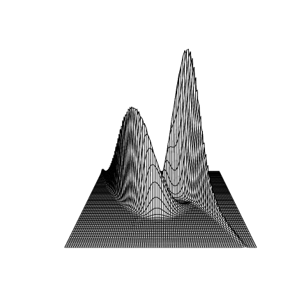
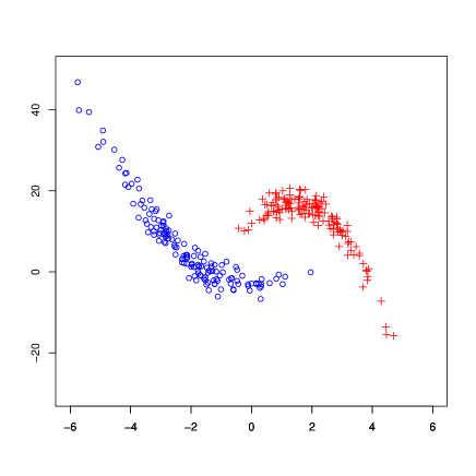
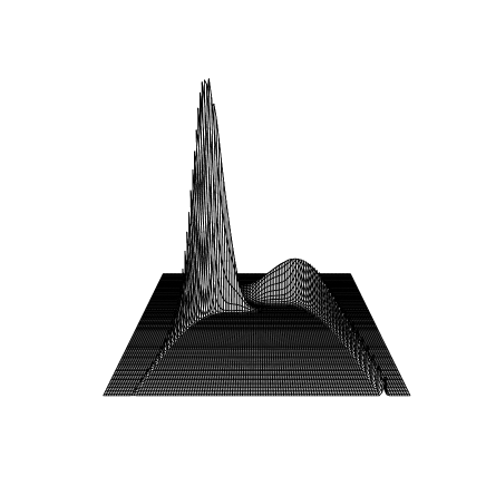
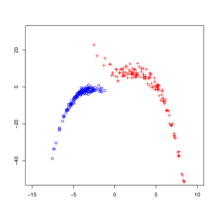
Figure 1: Two examples of Gaussian CWM densities and sample data based on quadratic (above) and cubic (below) mappings.

3.2 Finite Mixtures of Regression models

Secondly, Finite Mixtures of regression models (FMR) (DeSarbo and Cron, 1988; McLachlan and Peel, 2000; Frühwirth-Schnatter, 2005) are considered:

$$f(y|\mathbf{x};\mbox{\boldmath$\psi$})=\sum^{G}_{g=1}\phi(y;\mathbf{b}_{g}^{\prime}\mathbf{x}+b_{g0},\sigma^{2}_{\varepsilon,g})\,\pi_{g},$$ (11)

where vector $\psi$ denotes the overall parameters of the model. The posterior probability $p(\Omega_{g}|\mathbf{x},y)$ of the $g$-th group $(g=1,...,G)$ for FMR is:

$$p(\Omega_{g}|\mathbf{x},y)=\frac{f(y|\mathbf{x};\mbox{\boldmath$\psi$},\Omega_{g})}{f(y|\mathbf{x};\mbox{\boldmath$\psi$})}=\frac{\phi(y;\mathbf{b}_{g}^{\prime}\mathbf{x}+b_{g0},\sigma^{2}_{\varepsilon,g})\pi_{g}}{\sum^{G}_{j=1}\phi(y;\mathbf{b}_{j}^{\prime}\mathbf{x}+b_{j0},\sigma^{2}_{\varepsilon,j})\pi_{j}},\qquad g=1,\ldots,G\>$$ (12)

that is the classification of each observation depends on the local model and the mixing weight. We have the following result:

Proposition 2

Let us consider the linear Gaussian CWM (5), with $\mathbf{X}|\Omega_{g}\sim N_{d}(\mbox{\boldmath$\mu$}_{g},\mbox{\boldmath$\Sigma$}_{g})$ for $g=1,...,G$. If the probability density of $\mathbf{X}|\Omega_{g}$ does not depend on group $g$, i.e. $\phi_{d}(\mathbf{x};\mbox{\boldmath$\mu$}_{g},\mbox{\boldmath$\Sigma$}_{g})=\phi_{d}(\mathbf{x};\mbox{\boldmath$\mu$},\mbox{\boldmath$\Sigma$})$ for every $g=1,\ldots,G$, then it follows

$$p(\mathbf{x},y;\mbox{\boldmath$\theta$})=\phi_{d}(\mathbf{x};\mbox{\boldmath$\mu$},\mbox{\boldmath$\Sigma$})f(y|\mathbf{x};\mbox{\boldmath$\psi$})\;,$$

where $f(y|\mathbf{x};\mbox{\boldmath$\psi$})$ is the FMR model (11).

Proof. Assume that $\phi_{d}(\mathbf{x};\mbox{\boldmath$\mu$}_{g},\mbox{\boldmath$\Sigma$}_{g})=\phi_{d}(\mathbf{x};\mbox{\boldmath$\mu$},\mbox{\boldmath$\Sigma$})$, $g=1,\ldots,G$, then (5) yields:

$$p(\mathbf{x},y;\mbox{\boldmath$\theta$}) =\sum^{G}_{g=1}\phi(\mathbf{b}_{g}^{\prime}\mathbf{x}+b_{g0},\sigma^{2}_{\varepsilon,g})\,\phi_{d}(\mathbf{x};\mbox{\boldmath$\mu$},\mbox{\boldmath$\Sigma$})\,\pi_{g}$$

$$=\phi_{d}(\mathbf{x};\mbox{\boldmath$\mu$},\mbox{\boldmath$\Sigma$})\,\sum^{G}_{g=1}\phi(y;\mathbf{b}_{g}^{\prime}\mathbf{x}+b_{g0},\sigma^{2}_{\varepsilon,g})\,\pi_{g}$$

$$=\phi_{d}(\mathbf{x};\mbox{\boldmath$\mu$},\mbox{\boldmath$\Sigma$})\,\sum^{G}_{g=1}f(y|\mathbf{x};\mbox{\boldmath$\psi$})\pi_{g},$$

where $f(y|\mathbf{x};\mbox{\boldmath$\psi$})$ is FMR model (11). ∎

The second result of this section shows that, under the same hypothesis, CWM contains FMR.

Corollary 3

If the probability density of $\mathbf{X}|\Omega_{g}\sim N_{d}(\mbox{\boldmath$\mu$}_{g},\mbox{\boldmath$\Sigma$}_{g})$ in (5) does not depend on the group $g$, i.e. $\phi_{d}(\mathbf{x};\mbox{\boldmath$\mu$}_{g},\mbox{\boldmath$\Sigma$}_{g})=\phi_{d}(\mathbf{x};\mbox{\boldmath$\mu$},\mbox{\boldmath$\Sigma$})$ for every $g=1,\ldots,G$, then the posterior probability (6) coincides with (12).

Proof. Assume that $\phi_{d}(\mathbf{x};\mbox{\boldmath$\mu$}_{g},\mbox{\boldmath$\Sigma$}_{g})=\phi_{d}(\mathbf{x};\mbox{\boldmath$\mu$},\mbox{\boldmath$\Sigma$})$, $g=1,\ldots,G$, thus from (6) we get

$$p(\Omega_{g}|\mathbf{x},y) =\frac{\phi(y;\mathbf{b}_{g}^{\prime}\mathbf{x}+b_{g0},\sigma^{2}_{\varepsilon,g})\phi_{d}(\mathbf{x};\mbox{\boldmath$\mu$},\mbox{\boldmath$\Sigma$})\pi_{g}}{\sum^{G}_{j=1}\phi(y;\mathbf{b}_{j}^{\prime}\mathbf{x}+b_{j0},\sigma^{2}_{\varepsilon,j})\phi_{d}(\mathbf{x};\mbox{\boldmath$\mu$},\mbox{\boldmath$\Sigma$})\pi_{j}}=$$

$$=\frac{\phi(y;\mathbf{b}_{g}^{\prime}\mathbf{x}+b_{g0},\sigma^{2}_{\varepsilon,g})\phi_{d}(\mathbf{x};\mbox{\boldmath$\mu$},\mbox{\boldmath$\Sigma$})\pi_{g}}{\phi_{d}(\mathbf{x};\mbox{\boldmath$\mu$},\mbox{\boldmath$\Sigma$})\sum^{G}_{j=1}\phi(y;\mathbf{b}_{j}^{\prime}\mathbf{x}+b_{j0},\sigma^{2}_{\varepsilon,j})\pi_{j}}=$$

$$=\frac{\phi(y;\mathbf{b}_{g}^{\prime}\mathbf{x}+b_{g0},\sigma^{2}_{\varepsilon,g})\pi_{g}}{\sum^{G}_{j=1}\phi(y;\mathbf{b}_{j}^{\prime}\mathbf{x}+b_{j0},\sigma^{2}_{\varepsilon,j})\pi_{j}}$$

for $g=1,\ldots,G$, which coincides with (12). ∎

3.3 Finite Mixtures of Regression models with Concomitant variables

Finite Mixtures of Regression models with Concomitant variables (FMRC) (Dayton and Macready, 1988; Wedel, 2002) are an extension of FMR:

$$f^{*}(y|\mathbf{x};\mbox{\boldmath$\psi$}^{*})=\sum^{G}_{g=1}\phi(y;\mathbf{b}_{g}^{\prime}\mathbf{x}+b_{g0},\sigma^{2}_{\varepsilon,g})\,p(\Omega_{g}|\mathbf{x},\mbox{\boldmath$\xi$})\>,$$ (13)

where the mixing weight $p(\Omega_{g}|\mathbf{x},\mbox{\boldmath$\xi$})$ is a function depending on $\mathbf{x}$ through some parameters $\xi$ and $\mbox{\boldmath$\psi$}^{*}$ is the augmented set of all parameters of the model. The probability $p(\Omega_{g}|\mathbf{x},\mbox{\boldmath$\xi$})$ is usually modeled by a multinomial logistic distribution with the first component as baseline, that is:

$$p(\Omega_{g}|\mathbf{x},\mbox{\boldmath$\xi$}) =\frac{\exp(\mbox{\bf w}_{g}^{\prime}\mathbf{x}+w_{g0})}{\sum^{G}_{j=1}\exp(\mbox{\bf w}_{j}^{\prime}\mathbf{x}+w_{j0})}\,.$$ (14)

Equation (14) is satisfied by multivariate Gaussians of $\mathbf{X}$-distributions with the same covariance matrices, see e.g. Anderson (1972).

The posterior probability $p(\Omega_{g}|\mathbf{x},y)$ of the $g$-th group $(g=1,...,G)$ for FMRC is:

$$p(\Omega_{g}|\mathbf{x},y)=\frac{f^{*}(y|\mathbf{x};\mbox{\boldmath$\psi$}^{*},\Omega_{g})}{f^{*}(y|\mathbf{x};\mbox{\boldmath$\psi$}^{*})}=\frac{\phi(y;\mathbf{b}_{g}^{\prime}\mathbf{x}+b_{g0},\sigma^{2}_{\varepsilon,g}),\sigma_{\epsilon,g}^{2})p(\Omega_{g}|\mathbf{x},\mbox{\boldmath$\xi$})}{\sum_{j=1}^{G}\phi(y;\mathbf{b}_{j}^{\prime}\mathbf{x}+b_{j0},\sigma^{2}_{\varepsilon,j})p(\Omega_{j}|\mathbf{x},\mbox{\boldmath$\xi$})}.$$ (15)

Under suitable assumptions, linear Gaussian CWM leads to the same estimates of $\mathbf{b}_{g},b_{g0}$ ($g=1,\ldots,G$) in (13).

Proposition 4

Let us consider the linear Gaussian CWM (5), with $\mathbf{X}|\Omega_{g}\sim N_{d}(\mbox{\boldmath$\mu$}_{g},\mbox{\boldmath$\Sigma$}_{g})$ $(g=1,...,G)$. If $\mbox{\boldmath$\Sigma$}_{g}=\mbox{\boldmath$\Sigma$}$ and $\pi_{g}=\pi=1/G$ for every $g=1,\ldots,G$, then it follows

$$p(\mathbf{x},y;\mbox{\boldmath$\theta$})=p(\mathbf{x})f^{*}(y|\mathbf{x};\mbox{\boldmath$\psi$}^{*}),$$

where $f^{*}(y|\mathbf{x};\mbox{\boldmath$\psi$}^{*})$ is the FMRC model (13) based on the multinomial logistic (14) and $p(\mathbf{x})=\sum_{g=1}^{G}p(\mathbf{x}|\mbox{\boldmath$\Omega$}_{g})\pi_{g}$.

Proof. Assume $\mbox{\boldmath$\Sigma$}_{g}=\mbox{\boldmath$\Sigma$}$ and $\pi_{g}=\pi=1/G$ for every $g=1,\ldots,G$, thus the density (5) yields:

$$p(\mathbf{x},y;\mbox{\boldmath$\theta$}) =\sum^{G}_{g=1}\phi(\mathbf{b}_{g}^{\prime}\mathbf{x}+b_{g0},\sigma^{2}_{\varepsilon,g})\,\phi_{d}(\mathbf{x};\mbox{\boldmath$\mu$}_{g},\mbox{\boldmath$\Sigma$})\,\pi$$

$$=p(\mathbf{x})\sum^{G}_{g=1}\phi(\mathbf{b}_{g}^{\prime}\mathbf{x}+b_{g0},\sigma^{2}_{\varepsilon,g})\frac{\phi_{d}(\mathbf{x};\mbox{\boldmath$\mu$}_{g},\mbox{\boldmath$\Sigma$})\pi}{p(\mathbf{x})}$$

$$=p(\mathbf{x})\sum^{G}_{g=1}\phi(\mathbf{b}_{g}^{\prime}\mathbf{x}+b_{g0},\sigma^{2}_{\varepsilon,g})\frac{\exp\left[-\frac{1}{2}(\mathbf{x}-\mbox{\boldmath$\mu$}_{g})^{\prime}\mbox{\boldmath$\Sigma$}^{-1}(\mathbf{x}-\mbox{\boldmath$\mu$}_{g})\right]}{\sum_{j=1}^{G}\exp\left[-\frac{1}{2}(\mathbf{x}-\mbox{\boldmath$\mu$}_{j})^{\prime}\mbox{\boldmath$\Sigma$}^{-1}(\mathbf{x}-\mbox{\boldmath$\mu$}_{j})\right]}\,,$$

where

$$\frac{\exp\left[-\frac{1}{2}(\mathbf{x}-\mbox{\boldmath$\mu$}_{g})^{\prime}\mbox{\boldmath$\Sigma$}^{-1}(\mathbf{x}-\mbox{\boldmath$\mu$}_{g})\right]}{\sum_{j=1}^{G}\exp\left[-\frac{1}{2}(\mathbf{x}-\mbox{\boldmath$\mu$}_{j})^{\prime}\mbox{\boldmath$\Sigma$}^{-1}(\mathbf{x}-\mbox{\boldmath$\mu$}_{j})\right]}$$

$$\qquad=\frac{1}{1+\sum_{j\neq g}\exp\left[-\frac{1}{2}(\mathbf{x}-\mbox{\boldmath$\mu$}_{j})^{\prime}\mbox{\boldmath$\Sigma$}^{-1}(\mathbf{x}-\mbox{\boldmath$\mu$}_{j})+\frac{1}{2}(\mathbf{x}-\mbox{\boldmath$\mu$}_{g})^{\prime}\mbox{\boldmath$\Sigma$}^{-1}(\mathbf{x}-\mbox{\boldmath$\mu$}_{g})\right]}$$

$$\qquad=\frac{1}{1+\sum_{j\neq g}\exp\left[(\mbox{\boldmath$\mu$}_{j}-\mbox{\boldmath$\mu$}_{g})^{\prime}\mbox{\boldmath$\Sigma$}^{-1}\mathbf{x}-\frac{1}{2}(\mbox{\boldmath$\mu$}_{j}+\mbox{\boldmath$\mu$}_{g})^{\prime}\mbox{\boldmath$\Sigma$}^{-1}(\mbox{\boldmath$\mu$}_{j}-\mbox{\boldmath$\mu$}_{g})\right]}$$ (16)

and we recognize that (16) can be written in form (14) for suitable constants $\mbox{\bf w}_{g},w_{g0}$ ($g=1,\ldots,G$). This completes the proof. ∎

Based on similar arguments, we can immediately prove that, under the same hypotheses, CWM contains FMRC.

Corollary 5

Let us consider the linear Gaussian CWM (5). If $\mbox{\boldmath$\Sigma$}_{g}=\mbox{\boldmath$\Sigma$}$ and $\pi_{g}=\pi=1/G$ for every $g=1,\ldots,G$, then posterior probability (6) coincides with (15).

Proof. First, based on (14), let us rewrite (15) as

$$p(\Omega_{g}|\mathbf{x},y)=\frac{\phi(y;\mathbf{b}_{g}^{\prime}\mathbf{x}+b_{g0},\sigma^{2}_{\varepsilon,g})\exp(\mbox{\bf w}_{g}^{\prime}\mathbf{x}+w_{g0})}{\sum_{j=1}^{G}\phi(y;\mathbf{b}_{j}^{\prime}\mathbf{x}+b_{j0},\sigma^{2}_{\varepsilon,j})\exp(\mbox{\bf w}_{j}^{\prime}\mathbf{x}+w_{j0})}.$$ (17)

Assume $\mbox{\boldmath$\Sigma$}_{g}=\mbox{\boldmath$\Sigma$}$ and $\pi_{g}=\pi=1/G$ for every $g=1,\ldots,G$, thus from (4) and (6) we get

$$p(\Omega_{g}|\mathbf{x},y) =\frac{\phi(y;\mathbf{b}_{g}^{\prime}\mathbf{x}+b_{g0},\sigma^{2}_{\varepsilon,g})\phi_{d}(\mathbf{x};\mbox{\boldmath$\mu$}_{g},\mbox{\boldmath$\Sigma$})}{\sum^{G}_{j=1}\phi(y;\mathbf{b}_{j}^{\prime}\mathbf{x}+b_{j0},\sigma^{2}_{\varepsilon,j})\phi_{d}(\mathbf{x};\mbox{\boldmath$\mu$}_{j},\mbox{\boldmath$\Sigma$})}$$

and after some algebra we find a quantity like (17). This completes the proof. ∎

As for the relation between FMRC and linear Gaussian CWM, consider that the joint density $p(\mathbf{x},\Omega_{g})$ can be written in either form:

$$p(\mathbf{x},\Omega_{g})=p(\mathbf{x}|\Omega_{g})p(\Omega_{g})\qquad{\rm or}\qquad p(\mathbf{x},\Omega_{g})=p(\Omega_{g}|\mathbf{x})p(\mathbf{x})\>,$$ (18)

where quantity $p(\mathbf{x}|\Omega_{g})$ is involved in CWM (left-hand side), while FMRC contains conditional probability $p(\Omega_{g}|\mathbf{x})$ (right-hand side). In other words, CWM is a $\Omega_{g}$-to-$\mathbf{x}$ model, while FMRC is a $\mathbf{x}$-to-$\Omega_{g}$ model. According to Jordan (1995), in the framework of neural networks, they are called the generative direction model and the diagnostic direction model, respectively.

The results of this section are listed in Table 1, which summarizes the relationships between linear Gaussian CWM and traditional Gaussian mixture models.

model	$p(\mathbf{x}|\Omega_{g})$	$p(y|\mathbf{x},\Omega_{g})$	parameterisation of $\pi_{g}$	relationship	assumptions
FMG	Gaussian	Gaussian	none	linear
FMR	none	Gaussian	none	linear	$(\mbox{\boldmath$\mu$}_{g},\mbox{\boldmath$\Sigma$}_{g})=(\mbox{\boldmath$\mu$},\mbox{\boldmath$\Sigma$})$, g=1,…,G
FMRC	none	Gaussian	logistic	linear	$\mbox{\boldmath$\Sigma$}_{g}=\mbox{\boldmath$\Sigma$}$ and $\pi_{g}=\pi$, g=1,…,G

Table 1: Relationships between linear Gaussian CWM and traditional Gaussian mixtures.

Finally, we remark that if the conditional distributions $p(y|\mathbf{x},\Omega_{g})=\phi(y;\mathbf{b}_{g}^{\prime}\mathbf{x}+b_{g0},\sigma^{2}_{\varepsilon,g})$ ($g=1,\ldots,G$) do not depend on group $g$, that is $\phi(y;\mathbf{b}_{g}^{\prime}\mathbf{x}+b_{g0},\sigma^{2}_{\varepsilon,g})=\phi(y;\mathbf{b}^{\prime}\mathbf{x}+b_{0},\sigma^{2}_{\varepsilon})$ for $g=1,\ldots,G$, then (5) specializes as:

$$p(\mathbf{x},y;\mbox{\boldmath$\theta$}) =\sum^{G}_{g=1}\phi(y;\mathbf{b}_{g}^{\prime}\mathbf{x}+b_{g0},\sigma^{2}_{\varepsilon,g})\,\phi_{d}(\mathbf{x};\mbox{\boldmath$\mu$}_{g},\mbox{\boldmath$\Sigma$}_{g})\,\pi_{g}$$

$$=\phi(y;\mathbf{b}^{\prime}\mathbf{x}+b_{0},\sigma^{2}_{\varepsilon})\sum^{G}_{g=1}\,\phi_{d}(\mathbf{x};\mbox{\boldmath$\mu$}_{g},\mbox{\boldmath$\Sigma$}_{g})\,\pi_{g}\>,$$ (19)

and this implies that, from (11) and (13), FMR and FMRC are reduced to a single straight line:

$$f(y|\mathbf{x};\mbox{\boldmath$\psi$})=f^{*}(y|\mathbf{x};\mbox{\boldmath$\psi$}^{*})=\phi(y;\mathbf{b}^{\prime}\mathbf{x}+b_{0}),$$

since $\sum_{g=1}^{G}\pi_{g}=\sum_{g=1}^{G}p(\Omega_{g}|\mathbf{x},\mbox{\boldmath$\xi$})=1$. The results of this section will be illustrated from a numerical point of view in Section 5.1.

4 Student-$t$-CWM

In this section we introduce CWM based on Student-$t$ distributions. Data modeling according to the Student-$t$ distribution has been proposed in the literature in order to provide more robust fitting for groups of observations with longer than normal tails or atypical observations, see e.g. Zellner (1976); Lange et al. (1989); Bernardo and Girón (1992); McLachlan and Peel (1998, 2000); Peel and McLachlan (2000); Nadarajah and Kotz (2005). Recent applications include also analysis of orthodontic data via linear effect models (Pinheiro et al., 2001), marketing data analysis (Andrews et al., 2002) and asset pricing (Kan and Zhou, 2006).

To begin with, we recall that a $q$ variate random vector $\mathbf{Z}$ has a multivariate $t$ distribution with degrees of freedom $\nu\in(0,\infty)$, location parameter $\mbox{\boldmath$\mu$}\in\mathbb{R}^{q}$ and $q\times q$ positive definite inner product matrix $\Sigma$ if it has density

$$p(\mathbf{z};\mbox{\boldmath$\mu$},\mbox{\boldmath$\Sigma$},\nu)=\frac{\Gamma((\nu+q)/2)\nu^{\nu/2}}{\Gamma(\nu/2)|\pi\mbox{\boldmath$\Sigma$}|^{1/2}[\nu+\delta(\mathbf{z},\mbox{\boldmath$\mu$};\mbox{\boldmath$\Sigma$})]^{(\nu+q)/2}},$$ (20)

where $\delta(\mathbf{z},\mbox{\boldmath$\mu$};\mbox{\boldmath$\Sigma$})=(\mathbf{z}-\mbox{\boldmath$\mu$})^{\prime}\mbox{\boldmath$\Sigma$}^{-1}(\mathbf{z}-\mbox{\boldmath$\mu$})$ denotes the squared Mahalanobis distance between $\mathbf{z}$ and $\mu$, with respect to matrix $\Sigma$, and $\Gamma(\cdot)$ is the Gamma function. In this case we write $\mathbf{Z}\sim t_{q}(\mbox{\boldmath$\mu$},\mbox{\boldmath$\Sigma$},\nu)$, and it results $\mathbb{E}(\mathbf{Z})=\mbox{\boldmath$\mu$}$ (for $\nu>1$) and Cov$(\mathbf{Z})=\nu\mbox{\boldmath$\Sigma$}/(\nu-2)$ (for $\nu>2$). It is well known that, if $U$ is a random variable, independent of $\mathbf{Z}$, such that $\nu U$ has a chi-squared distribution with $\nu$ degrees of freedom, that is $\nu U\sim\chi^{2}_{\nu}$, then $\mathbf{Z}|(U=u)\sim N_{q}(\mbox{\boldmath$\mu$},\mbox{\boldmath$\Sigma$}/u)$.

Throughout this section we assume that $\mathbf{X}|\Omega_{g}$ has a multivariate $t$ distribution with location parameter $\mbox{\boldmath$\mu$}_{g}$, inner product matrix $\mbox{\boldmath$\Sigma$}_{g}$ and degrees of freedom $\nu_{g}$, that is $\mathbf{X}|\Omega_{g}\sim t_{d}(\mbox{\boldmath$\mu$}_{g},\mbox{\boldmath$\Sigma$}_{g},\nu_{g})$, and that $Y|\mathbf{x},\Omega_{g}$ has a $t$ distribution with location parameter $\mu(\mathbf{x};\mbox{\boldmath$\beta$}_{g})$, scale parameter $\sigma^{2}_{g}$ and degrees of freedom $\zeta_{g}$, that is $Y|\mathbf{x},\Omega_{g}\sim t(\mu(\mathbf{x};\mbox{\boldmath$\beta$}_{g}),\sigma^{2}_{g},\zeta_{g})$, $g=1,\ldots,G$. Thus (1) specializes as:

$$p(\mathbf{x},y;\mbox{\boldmath$\theta$})=\sum^{G}_{g=1}t(y;\mu(\mathbf{x};\mbox{\boldmath$\beta$}_{g}),\sigma^{2}_{g},\zeta_{g})\>t_{d}(\mathbf{x};\mbox{\boldmath$\mu$}_{g},\mbox{\boldmath$\Sigma$}_{g},\nu_{g})\,\pi_{g}\>,$$ (21)

and this model will be referred to as t-CWM. The special case in which $\mu(\mathbf{x};\mbox{\boldmath$\beta$}_{g})$ is a linear mapping will be called linear t-CWM:

$$p(\mathbf{x},y;\mbox{\boldmath$\theta$})=\sum^{G}_{g=1}t(y;\mathbf{b}^{\prime}_{g}\mathbf{x}+b_{g0},\sigma^{2}_{g},\zeta_{g})\,,\,\mathbf{t}_{d}(\mathbf{x};\mbox{\boldmath$\mu$}_{g},\mbox{\boldmath$\Sigma$}_{g},\nu_{g})\,\pi_{g}\>.$$ (22)

where, according to (20), $g=1,\ldots,G$, we have

$$t(y;\mathbf{b}^{\prime}_{g}\mathbf{x}+b_{g0},\sigma^{2}_{g},\zeta_{g}) =\frac{\Gamma((\nu_{g,y}+1)/2)\zeta_{g}^{\zeta_{g}/2}}{\Gamma(\nu_{g,y}/2)\sqrt{\pi\sigma_{\epsilon,g}^{2}}\{\zeta_{g}+[y-(\mathbf{b}_{g}^{\prime}\mathbf{x}+b_{g0})]^{2}/\sigma_{\epsilon,g}^{2}\}^{(\zeta_{g}+1)/2}}$$

$$t_{d}(\mathbf{x};\mbox{\boldmath$\mu$}_{g},\mbox{\boldmath$\Sigma$}_{g},\nu_{g}) =\frac{\Gamma((\nu_{g,\mathbf{x}}+q)/2))\nu_{g,\mathbf{x}}^{\nu_{g,\mathbf{x}}/2}}{\Gamma(\nu_{g,\mathbf{x}}/2)|\pi\mbox{\boldmath$\Sigma$}_{g}|^{1/2}\{\nu_{g}+\delta(\mathbf{x},\mbox{\boldmath$\mu$}_{g};\mbox{\boldmath$\Sigma$}_{g})\}^{(\nu_{g,\mathbf{x}}+q)/2}}.$$

Moreover, the posterior probability (3) specializes as:

$$p(\Omega_{g}|\mathbf{x},y)=\frac{t(y;\mathbf{b}^{\prime}_{g}\mathbf{x}+b_{g0},\sigma^{2}_{g},\zeta_{g})\mathbf{t}_{d}(\mathbf{x};\mbox{\boldmath$\mu$}_{g},\mbox{\boldmath$\Sigma$}_{g},\nu_{g})\pi_{g}}{\sum^{G}_{j=1}t(y;\mathbf{b}^{\prime}_{j}\mathbf{x}+b_{j0},\sigma^{2}_{j},\zeta_{j})\mathbf{t}_{d}(\mathbf{x};\mbox{\boldmath$\mu$}_{j},\mbox{\boldmath$\Sigma$}_{j},\nu_{j})\pi_{j}}\,,\qquad g=1,\ldots,G\>.$$

The following result implies that, differently from the Gaussian case, linear t-CWM is not a Finite Mixture of $t$-distributions (FMT).

Proposition 6

Let $\mathbf{Z}$ be a random vector defined on $\Omega=\Omega_{1}\cup\cdots\Omega_{G}$ with values in $\mathbb{R}^{d+1}$ and set $\mathbf{Z}=(\mathbf{X}^{\prime},Y)^{\prime}$ where $\mathbf{X}$ is a $d$-dimensional input vector and $Y$ is a random variable defined on $\Omega$. Assume that the density of $\mathbf{Z}=(\mathbf{X}^{\prime},Y)^{\prime}$ can be written in the form of a linear $t$-CWM (22), where $\mathbf{X}|\Omega_{g}\sim t_{d}(\mbox{\boldmath$\mu$}_{g},\mbox{\boldmath$\Sigma$}_{g},\nu_{g})$ and $Y|\mathbf{x},\Omega_{g}\sim t(\mu(\mathbf{x};\mbox{\boldmath$\beta$}_{g}),\sigma^{2}_{g},\zeta_{g})$, $g=1,\ldots,G$. If $\zeta_{g}=\nu_{g}+d$ and $\sigma^{*2}_{g}=\sigma^{2}_{g}[\nu_{g}+\delta(\mathbf{x};\mbox{\boldmath$\mu$}_{g},\mbox{\boldmath$\Sigma$}_{g})]/(\nu_{g}+d)$ then the linear t-CWM (22) coincides with a FMT for suitable parameters $\mathbf{b}_{g},b_{g0}$ and $\sigma^{2}_{g}$, $g=1,\ldots,G$.

Proof. Let $\mathbf{Z}$ be a $q$-variate random vector having multivariate $t$ distribution (20) with degrees of freedom $\nu\in(0,\infty)$, location parameter $\mu$ and positive definite inner product matrix $\Sigma$. If $\mathbf{Z}$ is partitioned as $\mathbf{Z}=(\mathbf{Z}^{\prime}_{1},\mathbf{Z}^{\prime}_{2})^{\prime}$, where $\mathbf{Z}_{1}$ takes values in $\mathbb{R}^{q_{1}}$ and $\mathbf{Z}_{2}$ in $\mathbb{R}^{q_{2}}=\mathbb{R}^{q-q_{1}}$, then $\mathbf{Z}$ can be written as

$$\mbox{\boldmath$\mu$}=\begin{pmatrix}\mbox{\boldmath$\mu$}_{1}\\ \mbox{\boldmath$\mu$}_{2}\end{pmatrix}\quad{\rm and}\quad\mbox{\boldmath$\Sigma$}=\begin{pmatrix}\mbox{\boldmath$\Sigma$}_{11}&\mbox{\boldmath$\Sigma$}_{12}\\ \mbox{\boldmath$\Sigma$}_{21}&\mbox{\boldmath$\Sigma$}_{22}\end{pmatrix}\>.$$

Hence, based on properties of the multivariate $t$ distribution, see e.g. Dickey (1967), Liu and Rubin (1995), it can be proved that:

$$\mathbf{Z}_{1}\sim t_{q_{1}}(\mbox{\boldmath$\mu$}_{1},\mbox{\boldmath$\Sigma$}_{11},\nu)\quad{\rm and}\quad\mathbf{Z}_{2}|\mathbf{z}_{1}\sim t_{q_{2}}(\mbox{\boldmath$\mu$}_{2|1},\mbox{\boldmath$\Sigma$}^{*}_{2|1},\nu+q_{1}),\>$$ (23)

where

$$\begin{split}\mbox{\boldmath$\mu$}_{2|1}&=\mbox{\boldmath$\mu$}_{2|1}(\mathbf{z}_{1})=\mbox{\boldmath$\mu$}_{2}+\mbox{\boldmath$\Sigma$}_{21}\mbox{\boldmath$\Sigma$}_{11}^{-1}(\mathbf{z}_{1}-\mbox{\boldmath$\mu$}_{1})\\ \mbox{\boldmath$\Sigma$}^{*}_{2|1}&=\mbox{\boldmath$\Sigma$}^{*}_{2|1}(\mathbf{z}_{1})=\frac{\nu+\delta(\mathbf{z}_{1};\mbox{\boldmath$\mu$}_{1},\mbox{\boldmath$\Sigma$}_{11})}{\nu+q_{1}}\mbox{\boldmath$\Sigma$}_{2|1},\>\end{split}$$ (24)

with $\mbox{\boldmath$\Sigma$}_{2|1}=\mbox{\boldmath$\Sigma$}_{22}-\mbox{\boldmath$\Sigma$}_{21}\mbox{\boldmath$\Sigma$}_{11}^{-1}\mbox{\boldmath$\Sigma$}_{12}$ and $\delta(\mathbf{z}_{1};\mbox{\boldmath$\mu$}_{1},\mbox{\boldmath$\Sigma$}_{11})=(\mathbf{z}_{1}-\mbox{\boldmath$\mu$}_{1})^{\prime}\mbox{\boldmath$\Sigma$}^{-1}_{11}(\mathbf{z}_{1}-\mbox{\boldmath$\mu$}_{1})$. In particular, if we set $\mathbf{Z}=(\mathbf{X}^{\prime},Y)^{\prime}$ then (22) coincides with a FMT if $\zeta_{g}=\nu_{g}+d$ and $\sigma^{*2}_{g}=\sigma^{2}_{g}[\nu_{g}+\delta(\mathbf{x};\mbox{\boldmath$\mu$}_{g},\mbox{\boldmath$\Sigma$}_{g})]/(\nu_{g}+d)$. ∎

In conclusion, we remark that (22) defines a wide family of densities which includes FMT and Finite Mixtures of Regression models with Student-$t$ errors (not proposed in the literature yet, as far as the authors know). A numerical analysis concerning a comparison between the classifications obtained by either FMT and linear $t$-CWM will be presented in Section 5.3.

5 Empirical studies

The statistical models introduced before have been evaluated on the grounds of many empirical studies based on both real and simulated datasets. The CWM parameters have been estimated by means of the EM algorithm according to the maximum likelihood approach; the routines have been implemented in R with different initialization strategies, in order to avoid local optima. This section is organized as follows. In Subsection 5.1 we consider a comparison among linear Gaussian CWM and FMR, FMRC; in Subsection 5.3 we consider a comparison between linear $t$-CWM and FMT; in Subsection 5.2 we present further numerical studies based on simulated data in order to evaluate model performance in the area of robust clustering; finally, in Subsection 5.4 we consider another case study concerning a real dataset in the medical area.

5.1 A comparison among linear Gaussian CWM and FMR, FMRC

To begin with, we present some simulation studies in order to verify empirically the theoretical results of Section 3, that is linear Gaussian CWM contains FMR and FMRC as special cases (in particular, data modeling via FMRC has been carried out by means of Flexmix R-package, see Leisch (2004)).

For this aim, we have considered some cases concerning classification of units $(x,y)\in\mathbb{R}^{2}$. The data have been obtained as follows: first, we have generated samples $\mathbf{x}_{1},\ldots,\mathbf{x}_{G}$ (corresponding to the $X$-variable) according to $G$ Gaussian distributions with parameters $(\mu_{g},\sigma^{2}_{g})$; each sample $\mathbf{x}_{g}$ has a size $N_{g}$, $(g=1,...,G)$. Afterwards, from $\mathbf{x}_{g}=(x_{g1},\ldots,x_{gN_{g}})^{\prime}$ we obtained vector $\mathbf{y}_{g}=(y_{g1},\ldots,y_{gN_{g}})^{\prime}$ considering realizations of the random variables $Y_{gn}=b_{g1}x_{gn}+b_{g0}+\epsilon_{g}$, for $g=1,\ldots,G$ and $n=1,\ldots,N_{g}$, where $b_{g1},b_{g0}\in\mathbb{R}$ and $\epsilon\sim N(0,\sigma^{2}_{\epsilon,g})$. Moreover, the obtained results according to CWM, FMR or FMRC have been compared by means of the following quantities :

1. The Wilks’s lambda $\Lambda$, which is used in multivariate analysis of variance, given by

   $$\Lambda=\frac{\mbox{det}\,\mathbf{W}}{\mbox{det}\,\mathbf{T}},$$ (25)

   where $\mathbf{T}$ is the total scatter matrix and $\mathbf{W}$ is the within-class scatter matrix:

   $$\mathbf{W}=\sum_{g=1}^{G}\sum_{n=1}^{N_{g}}(\mathbf{z}_{ng}-\bar{\mathbf{z}}_{g})(\mathbf{z}_{ng}-\bar{\mathbf{z}}_{g})^{\prime}\quad{\rm and}\quad\mathbf{T}=\sum_{g=1}^{G}\sum_{n=1}^{N_{g}}(\mathbf{x}_{ng}-\bar{\mathbf{z}})(\mathbf{z}_{ng}-\bar{\mathbf{z}})^{\prime},$$

   with $\mathbf{z}=(\mathbf{x},y)$ and $\bar{\mathbf{z}}_{g}=(\mathbf{\bar{x}}_{g},\bar{y}_{g})$ being the vector mean of the $g$-th group.

2. An index of weighted model fitting (IWF) $\mathcal{E}$ defined as:

   $$\mathcal{E}=\left(\frac{1}{N}\sum_{n=1}^{N}\left[y_{n}-\left(\sum_{g=1}^{G}\mu(\mathbf{x}_{n};\mbox{\boldmath$\beta$}_{g})p(\Omega_{g}|\mathbf{x}_{n},y_{n})\right)\right]^{2}\right)^{1/2}\>.$$ (26)

3. The misclassification rate $\eta$, that is the percentage of units being classified in the wrong class.

Example 1

Here we give an example in which the densities of $\mathbf{X}|\Omega_{g}$ are not the same, and we show that CWM outperforms FMR. For this aim, we considered a two groups data sample; the data have been generated according to the following parameters:

		$\phi(x;\mu_{i},\sigma^{2}_{g})$			$\phi(y;b_{g0}+b_{g1}x,\sigma^{2}_{\varepsilon,g})$
	$N_{g}$	$\mu_{g}$	$\sigma_{g}$		$b_{g0}$	$b_{g1}$	$\sigma_{\epsilon,g}$
Group 1	100	10	2		2	6	2
Group 2	200	$-10$	2		4	$-6$	2

where $\mu_{2}=-\mu_{1}$. Data are shown in Figure 2. The obtained results according to CWM and FMR are summarized in the following table:

	$\Lambda$	$\mathcal{E}$	$\eta$
CWM	0.0396	2.003	0.00%
FMR	0.2306	7.013	5.33%

The analysis shows that CWM leads to well separated groups ($\Lambda=0.0396$) where all units have been classified properly ($\eta=0.00\%$) and the local models $p(y|x,\Omega_{g})$ present a good fitting to data ($\mathcal{E}=2.003$). On the contrary, FMR presents a bad data fitting ($\mathcal{E}=7.013$) and it leads to groups being partially overlapped ($\Lambda=0.2306$), even if the misclassification rate is small ($\eta=5.33\%$). Finally, we remark that FMRC leads to the same classification of CWM. The scatter plots of data classified according to CWM and FMR are given in Figure 2.

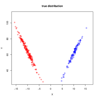
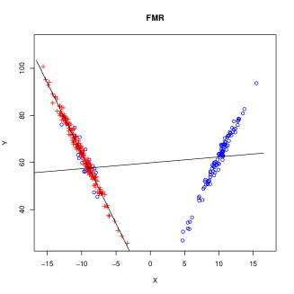
Figure 2: Example 1. True distribution, data classification and fitted lines according to CWM and FMR. The symbol $+$ denotes data classified in group 1 and $\circ$ denotes data classified in group 2.

Example 2

In order to illustrate a different situation, we consider another example in which the densities of $\mathbf{X}|\Omega_{g}$ are not the same. The data have been generated based on the following parameters:

		$\phi(x;\mu_{i},\sigma^{2}_{g})$			$\phi(y;b_{g0}+b_{g1}x,\sigma^{2}_{\varepsilon,g})$
	$N_{g}$	$\mu_{g}$	$\sigma_{g}$		$b_{g0}$	$b_{g1}$	$\sigma_{\epsilon,g}$
Group 1	100	5	1		40	6	2
Group 2	200	$10$	2		40	$-1.5$	1
Group 3	150	$20$	3		150	$7$	2

Data are shown in Figure 2. The obtained results according to CWM and FMR are summarized in the following table:

	$\Lambda$	$\mathcal{E}$	$\eta$
CWM	0.0498	1.678	0.00%
FMR	0.0909	1.647	8.67%

In this case, the analysis shows that CWM leads to well separated groups ($\Lambda=0.0498$) where all units have been classified properly ($\eta=0.00\%$) and the local models $p(y|x,\Omega_{g})$ present a good fitting to data ($\mathcal{E}=1.678$). Also FMR yields essentially the same conditional distributions ($\mathcal{E}=1.647$), but it presents a slightly worse value of the $\Lambda=0.0909$ and a misclassification rate $\eta=8.67\%$. Also in this case, we remark that FMRC attains the same classification of CWM. The scatter plots of data classified according to CWM and FMR are given in Figure 3.

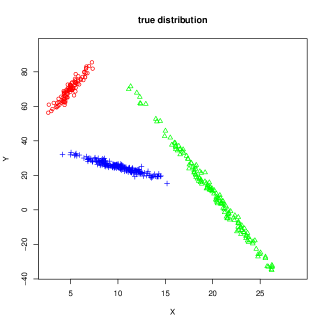
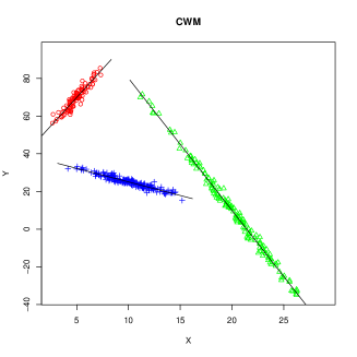
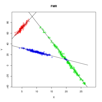
Figure 3: Example 2. Data classification and fitted lines according to CWM and FMR. The symbol $+$ denotes data classified in group 1, $\circ$ denotes data classified in group 2 and $\triangle$ denotes data classified in group 3.

Example 3

In the third example, we consider $G=3$ groups with the same conditional distributions; the data have been generated based on the following parameters:

		$\phi(x;\mu_{i},\sigma^{2}_{g})$			$\phi(y;b_{g0}+b_{g1}x,\sigma^{2}_{\varepsilon,g})$
	$N_{g}$	$\mu_{g}$	$\sigma_{g}$		$b_{g0}$	$b_{g1}$	$\sigma_{\epsilon,g}$
Group 1	100	5	2		2	6	2
Group 2	200	$20$	1		2	6	1
Group 3	150	$40$	2		2	6	2

Data are shown in Figure 4. The obtained results according to CWM, FMR and FMRC are summarized in the following table:

	$\Lambda$	$\mathcal{E}$	$\eta$
CWM	0.0146	1.678	0.00%
FMR	0.9782	2.25	51.33%
FMRC	0.9581	0.87	45.78%

As we can see, CWM perfectly identifies the three groups, while both FMR and FMRC lead to very bad results because the groups have the same conditional distributions. As a matter of fact, the reason is that the classification of CWM is based on both marginal and conditional distributions. The scatter plots of data classified according to CWM, FMR and FMRC are given in Figure 4.

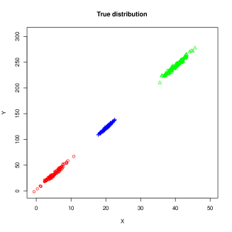
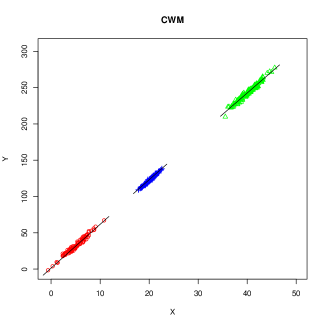
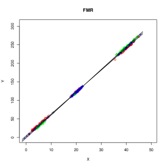
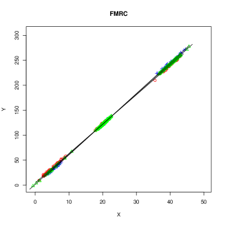
Figure 4: Example 3. True distribution and data classification and fitted lines according to CWM, FMR and FMRC. The symbol $+$ denotes data classified in group 1, $\circ$ denotes data classified in group 2 and $\triangle$ denotes data classified in group 3.

5.2 Robust clustering of noisy data

In this section we present the results of some numerical analysis concerning robust clustering from noisy simulated data. The data have been fitted according to a procedure based on three steps. First, we identify a subset $\mathcal{O}$ of units which are marked as outliers (i.e. noise data); secondly, we model the reduced dataset $\mathcal{D}^{\prime}=\mathcal{D}\setminus\mathcal{O}$ using CWM and estimate the parameters. Finally, based on such estimate, we classify the whole dataset $\mathcal{D}$ into $G$ groups plus a group of noise data.

The first step can be performed following different strategies. Once the estimates of the parameters of the $g$-th group ($g=1,\ldots,G$), have been obtained, consider the squared Mahalanobis distance between each unit and the $g$-th local estimate. In the framework of robust clustering via FMT, Peel and McLachlan (2000) proposed an approach based on the maximum likelihood; in particular, an observation $\mathbf{x}_{n}$ is treated as an outlier (and thus it will be classified as noise data) if

$$\sum_{g=1}^{G}\hat{z}_{jn}\delta(\mathbf{x}_{n};\hat{\mbox{\boldmath$\mu$}}_{g},\hat{\mbox{\boldmath$\Sigma$}}_{g})>\chi^{2}_{1-\alpha}(q)\,,$$

where $\hat{z}_{jn}=1$ if $\mathbf{x}_{n}$ unit is classified in the $j$-th group according to the maximum posterior probability and 0 otherwise, $\delta(\mathbf{x}_{n};\hat{\mbox{\boldmath$\mu$}}_{g},\hat{\mbox{\boldmath$\Sigma$}}_{g})=(\mathbf{x}_{n}-\hat{\mbox{\boldmath$\mu$}}_{g})^{\prime}\hat{\mbox{\boldmath$\Sigma$}}_{g}^{-1}(\mathbf{x}_{n}-\hat{\mbox{\boldmath$\mu$}}_{g})$ and $\chi^{2}_{1-\alpha}(q)$ denotes the quantile of order $(1-\alpha)$ of the chi-squared distribution with $q$ degrees of freedom. More recent approaches are based on the forward search, see e.g. Riani et al. (2008), Riani et al. (2009), maximum likelihood estimation with a trimmed sample, see Cuesta-Albertos et al. (2008), Gallegos and Ritter (2009), Gallegos and Ritter (2009b) and on multivariate outlier tests based on the minimum covariance determinant estimator, see Cerioli (2010).

For the scope of the present paper, we followed Peel and McLachlan (2000)’s strategy, using a Student-$t$ CWM. Cluster Weighted Modeling of noisy data according to other strategies provides ideas for further research.

As far as the second step is concerned, the parameters have been estimated once the reduced dataset $\mathcal{D}^{\prime}=\mathcal{D}\setminus\mathcal{O}$ according to either Gaussian or Student-$t$ CWM has been obtained. In the following, such strategies will be referred to as Student-Gaussian CWM (tG-CWM) and Student-Student CWM (tt-CWM), respectively. Finally the data have been classified into $G+1$ groups. A similar strategy has also been considered in Greselin and Ingrassia (2010).

Example 4 (Gaussian simulated data with noise.)

The first simulated dataset concerns a sample of 300 units generated according to (5) with $G=3$, $d=1$, $\pi_{1}=\pi_{2}=\pi_{3}=1/3$. The parameters are listed in the following table for two different values of $\sigma=\sigma_{\epsilon}=2$ and $\sigma=\sigma_{\epsilon}=4$

		$\phi(x;\mu_{i},\sigma^{2}_{g})$			$\phi(y;b_{g0}+b_{g1}x,\sigma^{2}_{\varepsilon,g})$
	$N_{g}$	$\mu_{g}$	$\sigma_{g}$		$b_{g0}$	$b_{g1}$	$\sigma_{\epsilon,g}$
Group 1	100	5	$\sigma$		40	$6$	$\sigma_{\epsilon}$
Group 2	100	$10$	$\sigma$		40	$-1.5$	$\sigma_{\epsilon}$
Group 3	100	$20$	$\sigma$		150	$-7$	$\sigma_{\epsilon}$

The sample data $\{(x_{n},y_{n})\}_{n=1,\ldots,300}$ have been obtained as follows: first, we have generated the samples $\mathbf{x}_{1},\ldots,\mathbf{x}_{N}$ according to $G=3$ Gaussian distributions with parameters $(\mu_{g},\sigma_{g})$, $g=1,...,G$. Afterwards, for each $x_{g}$ we generated the value $y_{g}$ (corresponding to the $Y$-variable) according to a Gaussian distribution with mean $b_{g0}+b_{g1}x$ and variance $\sigma^{2}_{\epsilon}$. Then, the above data set has been augmented by including a sample of 50 points generated with a uniform distribution in the rectangle $[-5,30]\times[-50,130]$ in order to simulate noise. Thus, the whole dataset $\mathcal{D}$ contains $N=350$ units, see Figure 5.

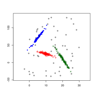
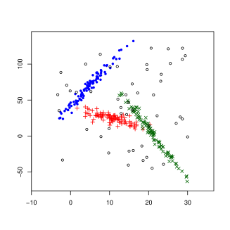
a)	b)

Figure 5: Example 4: a) data with $\sigma=2$, b) data with $\sigma=4$ (circles represent noise)

The results have been summarized in Table 2. tG-CWM and tt-CWM have in practice the same performance. In the case $\sigma=2$, tt-CWM slightly outperformed tG-CWM (the misclassification rates were $\eta=6.00\%$ and $\eta=5.71\%$, respectively); however, tt-CWM recognized a larger number of outliers than tG-CWM, viceversa in the case $\sigma=4$ we observed $\eta=4.29\%$ and $\eta=5.71\%$, respectively. We remark that the smallest misclassification error $\eta$ corresponds to the model with the smallest mean squared error $\mathcal{E}$.

a) Student-Gaussian CWM
estimated true 1 2 3 outlier 1 98 0 0 2 2 0 97 0 3 3 0 0 100 0 outlier 1 0 15 34		estimated true 1 2 3 outlier 1 99 0 0 1 2 0 98 1 1 3 0 1 99 0 outlier 5 2 4 39
case $\sigma=2$: $\mathcal{E}=7.97,\eta=6.00\%$		case $\sigma=4$: $\mathcal{E}=4.34,\eta=4.29\%$
b) Student-Student CWM
estimated true 1 2 3 outlier 1 94 0 0 6 2 0 92 0 8 3 0 0 99 1 outlier 1 0 4 45		estimated true 1 2 3 outlier 1 98 0 0 2 2 0 93 4 3 3 0 0 100 0 outlier 4 0 7 39
case $\sigma=2$: $\mathcal{E}=2.97,\eta=5.71\%$		case $\sigma=4$: $\mathcal{E}=5.8,\eta=5.71\%$

Table 2: Summary of the results concerning Example 4: confusion matrices, mean squared error and misclassification rate for data fitting using both Student-Gaussian CWM and Student-Student CWM. The smallest misclassification error has been attained in correspondence with the smallest value of $\mathcal{E}$.

Example 5 (Gaussian simulated data with noise.)

The second simulated example concerns a data set of size $150$ generated according to model (5) with $G=3$, $d=1$, $\pi_{1}=\pi_{2}=\pi_{3}=1/3$. The parameters are listed in the following table for two different values of $\sigma=\sigma_{\epsilon}=2$ and $\sigma=\sigma_{\epsilon}=4$:

		$\phi(x;\mu_{i},\sigma^{2}_{g})$			$\phi(y;b_{g0}+b_{g1}x,\sigma^{2}_{\varepsilon,g})$
	$N_{g}$	$\mu_{g}$	$\sigma_{g}$		$b_{g0}$	$b_{g1}$	$\sigma_{\epsilon,g}$
Group 1	100	5	$\sigma$		2	$6$	$\sigma_{\epsilon}$
Group 2	100	$10$	$\sigma$		2	$-1.5$	$\sigma_{\epsilon}$
Group 3	100	$40$	$\sigma$		2	$-7$	$\sigma_{\epsilon}$

i.e. the data are divided into $G=3$ groups along one straigth line. Afterwards, we added to the previous data a sample of 25 points generated by a uniform distribution in the rectangle $[-5,30]\times[-50,130]$ in order to simulate noise. Thus, $\mathcal{D}$ contains $N=175$ units, see Figure 6.

The results have been summarized in Table 3. In the case $\sigma=2$, tG-CWM slightly outperformed tt-CWM, the misclassification rates were $\eta=4.00\%$ and $\eta=5.14\%$, respectively; in the case $\sigma=4$ tG-CWM essentially identifies two groups (and thus $\eta=40\%$), while tt-CWM recognized the three groups with a misclassification rate $\eta=8.00\%$. Figure 6b) explains the reason for the relevant misclassification error in data fitting via tG-CWM: as a matter of fact two clusters are very close; in this case, tG-CWM identifies such two clusters as a whole, while tt-CWM correctly separates them. We point out that also in this case the smallest misclassification error $\eta$ corresponds to the model with the smallest mean squared error $\mathcal{E}$.

a) Student-Gaussian CWM
estimated true 1 2 3 outlier 1 47 0 0 3 2 0 50 0 1 3 0 0 49 1 outlier 0 2 1 22		estimated true 1 2 3 outlier 1 0 50 0 0 2 4 50 0 0 3 0 0 50 4 outlier 19 0 1 5
case $\sigma=2$: $\mathcal{E}=2.29,\eta=4.00\%$		case $\sigma=4$: $\mathcal{E}=71.39,\eta=40.00\%$
b) Student-Student CWM
estimated true 1 2 3 outlier 1 46 0 0 4 2 0 49 0 1 3 0 0 48 2 outlier 0 1 1 23		estimated true 1 2 3 outlier 1 49 0 0 1 2 4 46 0 0 3 0 0 46 4 outlier 0 0 5 20
case $\sigma=2$: $\mathcal{E}=7.25,\eta=5.14\%$		case $\sigma=4$: $\mathcal{E}=31.96,\eta=8.00\%$

Table 3: Summary of the results concerning Example 5: confusion matrices, mean squared error and misclassification rate for data fitting using both Student-Gaussian CWM and Student-Student CWM. The smallest misclassification error is obtained corresponding to the smallest value of $\mathcal{E}$.

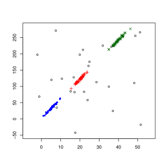
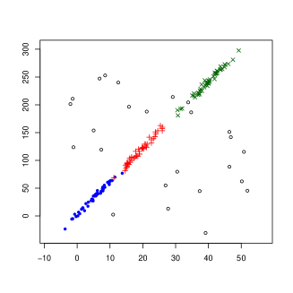
a)	b)

Figure 6: Example 5: a) data with $\sigma=2$, b) data with $\sigma=4$ (circles represent noise)

Example 6 (Bivariate Linear Gaussian simulated noisy data.)

The third example concerns a data set of size $300$ generated according again to (5) with $G=2$, $d=2$, $\pi_{1}=\pi_{2}=1/2$ with the following parameters for $p(y|\mathbf{x},\Omega_{g})$:

$$\mu(\mathbf{x},\mbox{\boldmath$\beta$}_{1})=6x_{1}+1.2x_{2}\qquad{\rm and}\qquad\mu(\mathbf{x},\mbox{\boldmath$\beta$}_{2})=-1.5x_{1}+3x_{2}$$

that is $\mbox{\boldmath$\mu$}_{1}=(6,1.2)^{\prime}$ and $\mbox{\boldmath$\mu$}_{2}=(-1.5,3)^{\prime}$, and the following parameters for $p(\mathbf{x}|\Omega_{g})=\phi_{2}(\mathbf{x};\mbox{\boldmath$\mu$}_{g},\mbox{\boldmath$\Sigma$}_{g})$, $g=1,2$, for two different values of $\sigma_{1}=\sigma_{2}=\sigma$ and $\sigma_{\epsilon,1}=\sigma_{\epsilon,2}=\sigma_{\epsilon}$, i.e. $\sigma=\sigma_{\epsilon}=2$ and $\sigma=\sigma_{\epsilon}=4$:

$$\mbox{\boldmath$\mu$}_{1}=(5,20)^{\prime}\;,\quad\mbox{\boldmath$\Sigma$}_{1}=\begin{pmatrix}4&-0.1\\ -0.1&4\end{pmatrix}\qquad{\rm and}\qquad\mbox{\boldmath$\mu$}_{2}=(2,4)\;,\quad\mbox{\boldmath$\Sigma$}_{2}=\begin{pmatrix}4&0.1\\ 0.1&4\end{pmatrix}$$

Afterwards, a sample of 50 points generated by a uniform distribution in the rectangle $[-5,40]\times[-5,40]\times[-20,170]$ has been added in order to simulate noise. Thus, the dataset $\mathcal{D}$ contains $N=350$ units. The results have been summarized in Table 4. In the case $\sigma=2$, tG-CWM slightly outperformed tt-CWM, the misclassification rates were $\eta=2.00\%$ and $\eta=2.29\%$, respectively; similar results we obtained in the case $\sigma=4$, where we got $\eta=6.57\%$ and $\eta=7.43\%$, respectively. Again the smallest misclassification error $\eta$ has been attained corresponding to the model with the smallest mean squared error $\mathcal{E}$.

a) Student-Gaussian CWM
estimated true 1 2 outlier 1 149 0 1 2 0 144 6 outlier 0 0 50		estimated true 1 2 outlier 1 149 1 0 2 0 145 5 outlier 0 2 48
case $\sigma=2$: $\mathcal{E}=2.08,\eta=2.00\%$		case $\sigma=4$: $\mathcal{E}=2.32,\eta=6.57\%$
b) Student-Student CWM
estimated true 1 2 outlier 1 139 0 11 2 0 138 12 outlier 0 0 50		estimated true 1 2 outlier 1 140 1 9 2 0 135 15 outlier 0 1 49
case $\sigma=2$: $\mathcal{E}=3.94,\eta=2.29\%$		case $\sigma=4$: $\mathcal{E}=4.64,\eta=7.43\%$

Table 4: Summary of the results concerning Example 6 (data with noise): confusion matrices, mean squared error and misclassification rate for data fitting using both Student-Gaussian CWM and Student-Student CWM. The smallest misclassification error is obtained corresponding to the smallest value of $\mathcal{E}$.

5.3 A comparison between linear $t$-CWM and FMT in robust clustering

In this section we present the results concerning robust classification via FMT and linear $t$-CWM (22) based on a real data set studied in Campbell and Mahon (1974) about rock crabs of the genus Leptograpsus (available at http://www.stats.ox.ac.uk/pub/PRNN/). Each specimen has five measurements (expressed in $mm$): width of the frontal lip (FL), rear width (RW), length along the mid line (CL) and maximum width (CW) of the carapace and body depth (BD); the data are grouped into two classes by sex, see Figure 7. According to the classes of application of CWM introduced in Section 2, this case study concerns a direct application of type B; in particular, in (22) the variable CL has been selected as the $Y$-variable. In the setting of FMT, this data set has been used in McLachlan and Peel (2000), Peel and McLachlan (2000) and in Liu et al. (2004). According to such references, here we cluster a sample of 100 units (with $n_{1}=50$ males and $n_{2}=50$ females) ignoring their true classification.

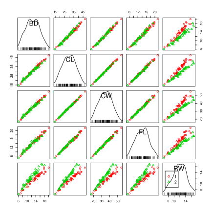
Figure 7: Scatterplot matrix of the crab data set.

The simulations have been performed along the lines of McLachlan and Peel (2000), Peel and McLachlan (2000). Outliers have been inserted in the original data set by adding a constant to the second variate of the 25th data point. In Table 5 the overall misclassification error is reported, comparing both FMT and linear $t$-CWM error rates obtained in the best case. We read Table 5 beginning from the central row, where the initial data set is considered (without any perturbation, as the constant value is null). Linear $t$-CWM outperformed FMT. Then, scanning the following rows of the table, the value of the constant raises progressively from 5 to 20 $mm$ and the error rate grows more slowly for FMT (reaching only 20%), while it remains almost unchanged for CWM.

Table 5: Comparison of error rates when fitting FMT and $t$-CWM to the crab data set with outliers. Variable CL has been selected as the $Y$-variable.

	FMT	linear $t$-CWM
Constant	Error Rate	Error Rate
$-15$	19%	13%
$-10$	19%	13%
$-5$	20%	13%
0	18%	12%
5	20%	12%
10	20%	11%
15	20%	12%
20	20%	12%

Finally, we remark that misclassification error rates obtained via linear $t$-CWM are equivalent to those obtained in Greselin and Ingrassia (2010) using suitable constraints on the eigenvalues of the covariance matrices of the two groups.

5.4 A case study in the medical area

Example 7 (Plasma Concentration of Beta-Carotene)

The last example concerns a case study based on real data about Beta-Carotene plasma levels described in Nierenberg et al. (1989). The data have been recently modeled in Schlattmann (2009) by using FMR and here we compare such approach with CWM. Our analysis concentrates on the relationship between Beta-Carotene plasma level and the amount of Beta-Carotene in the diet using a subset of $N=144$ individuals, with status ‘male’ and ‘never smoker’. Moreover, following the schema in Schlattmann (2009), we considered $G=4$ groups.

To begin with, we remark that the BIC criterion assumes a slightly smaller value for CWM (4298.6) rather than FMR (4324.5), see also Table 6 (we can compare the two values because FMR can be regarded as a nested model of CWM, see Section 3.2). Moreover, Gaussian CWM leads to better separated groups ($\Lambda=0.0934$) than FMR ($\Lambda=0.2655$); on the contrary, the index of weighted model fitting for CWM ($\mathcal{E}=70.3925$) attains a slightly worse value than FMR ($\mathcal{E}=54.1186$); however, considering the range of values of Beta-Carotene plasma level, this difference is not relevant and the fitting may be considered good in both cases. Figure 8 shows the classifications obtained by means of FMR and Gaussian CWM, respectively. Finally, the parameter estimates are reported in Table 7, where in parenthesis the standard error of the estimates are given. FMR classifies individuals into four straight lines along the dietary Beta-Carotene axis (see Figure 8). The effect of dietary Beta-Carotene is rather small in the first subpopulation ($b_{11}=0.0032$), a little greater in the second and fourth subpopulations ($b_{21}=0.0301$ and $b_{41}=0.0419$), whereas it is much larger in the third subpopulation ($b_{31}=0.2572$). Gaussian CWM produces a different classification, which takes into account the distribution of dietary Beta-Carotene (see Figure 8); in particular, a subpopulation with a negative relationship between Beta-Carotene plasma level and dietary Beta-Carotene ($b_{21}=-0.0393$) is identified.

In order to complete the data analysis, first we remark that the histogram of data concerning the amount of Beta-Carotene in the diet ($X$-variable) shows that the population is heterogeneous with respect to the independent variable, see Figure 9. This heterogeneity can be captured by CWM (which models the joint distribution) but not by FMR (which models only the conditional distribution). Secondly, we point out that group 2 in CWM exhibits a negative slope ($b_{21}=-0.0393$), while FMR leads to a model with all positive slopes. The identification of a subpopulation which negatively reacts to dietary Beta-Carotene seems to confirm the recent adverse findings about the effect of antioxidants intake on the incidence of lung cancer, see Schlattmann (2009) p.11. This might be a starting point for further investigations in the biomedical area.

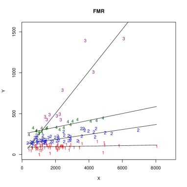
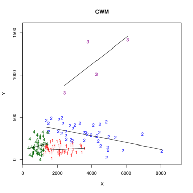
Figure 8: Betaplasma data: classification according to FMR and CWM.

Figure 9: Betaplasma data: Histogram of the amount of Beta-Carotene ($x$-variable).

	Gaussian CWM	FMR
$BIC$	4298.6	4324.5
$\Lambda$	0.0934	0.2655
$\mathcal{E}$	70.38	54.11

Table 6: Betaplasma data: values of BIC, $\Lambda$ and $\mathcal{E}$ for both Gaussian CWM and FMR.

group	parameters	Gaussian CWM	FMR
1	$\pi_{1}$	0.4036	0.3917
	$b_{10}$	103.0155 (2.2870)	89.9892 (1.0669)
	$b_{11}$	0.0087 (0.0011)	0.0032 (0.0004)
2	$\pi_{2}$	0.2789	0.3852
	$b_{20}$	436.1387 (5.1796)	125.4027 (1.4870)
	$b_{21}$	-0.0393 (0.0014)	0.0301 (0.0006)
3	$\pi_{3}$	0.0283	0.1016
	$b_{30}$	486.4574 (25.6135)	-11.9203 (9.5508)
	$b_{31}$	0.1590 (0.0058)	0.2572 (0.0033)
4	$\pi_{4}$	0.2893	0.1215
	$b_{40}$	112.1419 (5.1502)	249.8431 (1.6601)
	$b_{41}$	0.0524 (0.0051)	0.0419 (0.0006)

Table 7: Betaplasma: mixing weights and parameter estimates of the modes for both Gaussian CWM and FMR. In parenthesis the standard errors of the estimtes are given.

6 Concluding remarks

In this paper, we presented a statistical analysis of Cluster-Weighted Modeling (CWM) based on elliptical distributions. Under the Gaussian case a detailed comparison among CWM and some competitive local statistical models such mixtures of distributions and mixtures of regression models. Moreover, based on both analytical and geometrical arguments, we have shown that CWM can be regarded as a generalization of such models. We remark also that Proposition 2 could be extended to Finite Mixtures of Generalized Linear Models. Further, our numerical simulations showed that CWM provides a very flexible and powerful framework in data classification, useful to perform a suitable data fitting. Moreover, with respect to the comparison with FMR and FMRC, Wedel (2002) points out that assuming a distribution for the covariates makes inferences valid under repeated sampling and the model better suited to deal with general patterns of missing observations.

In the second part of the paper, we introduced new Cluster Weighted Modeling based on the Student-$t$ distribution for robust clustering. In this context, in fitting noisy data, we considered a procedure for removing noise and estimating the parameters of the model on the remaining data following an approach proposed in Peel and McLachlan (2000). In this framework, recent literature on robust parameter estimation provides ideas for further research.

Another important issue, which deserves attention for further research, concerns computational aspects of the parameter estimation in CWM. Parameters in CWM have been here estimated according to the maximum likelihood approach by means of the EM algorithm. In this paper, we have not presented a detailed analysis of the behaviour of the EM algorithm under different conditions. However, our numerical simulations confirmed the findings of Faria and Soromenho (2010) in fitting mixtures of linear regressions and we point out that the initialization of the algorithms is quite critical. In our simulations the initial guess has been made according to either a preliminary clustering of data using a $k$-means algorithm or a random grouping of data, but our numerical studies pointed out that there is no overwhelming strategy. Finally, we remark that, in order to reduce such critical aspects, suitable constraints on the eigenvalues of the covariance matrices could be implemented, see e.g. Ingrassia (2004), Ingrassia and Rocci (2007), Greselin and Ingrassia (2010). This provides other ideas for future work.

Appendix: Decision surfaces of CWM

The potentiality of CWM as a general framework can be illustrated also from a geometric point of view, by considering the decision surfaces which separate the clusters. In the following we will discuss the binary case, and in this case the decision surface is the set of $(\mathbf{x},y)\in\mathbb{R}^{d+1}$ such that $p(\Omega_{0}|\mathbf{x},y)=p(\Omega_{1}|\mathbf{x},y)=0.5$. Given that $p(\mathbf{x}|\Omega_{g})\pi_{g}=p(\Omega_{g}|\mathbf{x})p(\mathbf{x})$, we can rewrite $p(\Omega_{1}|\mathbf{x},y)$ as:

$$p(\Omega_{1}|\mathbf{x},y) =\frac{p(y|\mathbf{x},\Omega_{1})p(\Omega_{1}|\mathbf{x})}{p(y|\mathbf{x},\Omega_{0})p(\Omega_{0}|\mathbf{x})+p(y|\mathbf{x},\Omega_{1})p(\Omega_{1}|\mathbf{x})}=\frac{1}{1+\displaystyle{\frac{p(y|\mathbf{x},\Omega_{0})p(\Omega_{0}|\mathbf{x})}{p(y|\mathbf{x},\Omega_{1})p(\Omega_{1}|\mathbf{x})}}}$$

$$=\frac{1}{1+\exp\left\{-\ln\displaystyle{\frac{p(y|\mathbf{x},\Omega_{1})}{p(y|\mathbf{x},\Omega_{0})}}-\ln\displaystyle{\frac{p(\Omega_{1}|\mathbf{x})}{p(\Omega_{0}|\mathbf{x})}}\right\}}\>.$$ (27)

Thus it results $p(\Omega_{1}|\mathbf{x},y)=0.5$ when

$$\ln\frac{p(y|\mathbf{x},\Omega_{1})}{p(y|\mathbf{x},\Omega_{0})}+\ln\frac{p(\Omega_{1}|\mathbf{x})}{p(\Omega_{0}|\mathbf{x})}=0\>,$$

which may be rewritten as:

$$\ln\frac{p(y|\mathbf{x},\Omega_{1})}{p(y|\mathbf{x},\Omega_{0})}+\ln\frac{p(\mathbf{x}|\Omega_{1})}{p(\mathbf{x}|\Omega_{0})}+\ln\frac{\pi_{1}}{\pi_{0}}=0\>.$$ (28)

In the linear Gaussian CWM, the first and the second term in (28) are, respectively:

$$\ln\displaystyle{\frac{p(y|\mathbf{x},\Omega_{1})}{p(y|\mathbf{x},\Omega_{0})}} =\ln\frac{\sqrt{2\pi\sigma_{\epsilon,0}^{2}}}{\sqrt{2\pi\sigma_{\epsilon,1}^{2}}}+\frac{(y-\mathbf{b}_{0}^{\prime}\mathbf{x}-b_{00})^{2}}{2\sigma_{\epsilon,0}^{2}}-\frac{(y-\mathbf{b}_{1}^{\prime}\mathbf{x}-b_{10})^{2}}{2\sigma_{\epsilon,1}^{2}}\>$$

$$\ln\frac{p(\mathbf{x}|\Omega_{1})}{p(\mathbf{x}|\Omega_{0})} =\frac{1}{2}\ln\frac{|\mbox{\boldmath$\Sigma$}_{0}|}{|\mbox{\boldmath$\Sigma$}_{1}|}+\frac{1}{2}\left[(\mathbf{x}-\mbox{\boldmath$\mu$}_{0})^{\prime}\mbox{\boldmath$\Sigma$}_{0}^{-1}(\mathbf{x}-\mbox{\boldmath$\mu$}_{0})-(\mathbf{x}-\mbox{\boldmath$\mu$}_{1})^{\prime}\mbox{\boldmath$\Sigma$}_{1}^{-1}(\mathbf{x}-\mbox{\boldmath$\mu$}_{1})\right]\>.$$

Then, equation (28) is satisfied for $(\mathbf{x},y)\in\mathbb{R}^{d+1}$ such that:

$$\ln\frac{\sigma_{\epsilon,0}}{\sigma_{\epsilon,1}}+\frac{(y-\mathbf{b}_{0}^{\prime}\mathbf{x}-b_{00})^{2}}{2\sigma_{\epsilon,0}^{2}}-\frac{(y-\mathbf{b}_{1}^{\prime}\mathbf{x}-b_{10})^{2}}{2\sigma_{\epsilon,1}^{2}}+\frac{1}{2}\ln\frac{|\mbox{\boldmath$\Sigma$}_{0}|}{|\mbox{\boldmath$\Sigma$}_{1}|}+\\ \frac{1}{2}\left[(\mathbf{x}-\mbox{\boldmath$\mu$}_{0})^{\prime}\mbox{\boldmath$\Sigma$}_{0}^{-1}(\mathbf{x}-\mbox{\boldmath$\mu$}_{0})-(\mathbf{x}-\mbox{\boldmath$\mu$}_{1})^{\prime}\mbox{\boldmath$\Sigma$}_{1}^{-1}(\mathbf{x}-\mbox{\boldmath$\mu$}_{1})\right]+\ln\frac{\pi_{1}}{\pi_{0}}=0\>,$$ (29)

which defines quadratic surfaces, i.e. quadrics. Examples of quadrics are spheres, circular cylinders, and circular cones. In Figure 10, we give two examples of surfaces generated by (29).

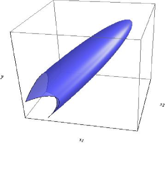
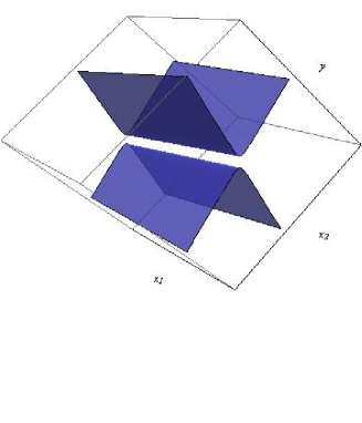
Figure 10: Examples of decision surfaces for linear Gaussian CWM (heteroscedastic case).

In the homoscedastic case $\mbox{\boldmath$\Sigma$}_{0}=\mbox{\boldmath$\Sigma$}_{1}=\mbox{\boldmath$\Sigma$}$ it is well known that:

$$\ln\frac{p(\mathbf{x}|\Omega_{1})}{p(\mathbf{x}|\Omega_{0})} =\frac{1}{2}\left[(\mathbf{x}-\mbox{\boldmath$\mu$}_{0})^{\prime}\mbox{\boldmath$\Sigma$}^{-1}(\mathbf{x}-\mbox{\boldmath$\mu$}_{0})-(\mathbf{x}-\mbox{\boldmath$\mu$}_{1})^{\prime}\mbox{\boldmath$\Sigma$}^{-1}(\mathbf{x}-\mbox{\boldmath$\mu$}_{1})\right]$$

$$=\mbox{\bf w}^{\prime}\mathbf{x}+w_{0},$$ (30)

where

$$\mbox{\bf w}=\mbox{\boldmath$\Sigma$}^{-1}(\mbox{\boldmath$\mu$}_{1}-\mbox{\boldmath$\mu$}_{0})\quad{\rm and}\quad w_{0}=\frac{1}{2}(\mbox{\boldmath$\mu$}_{0}+\mbox{\boldmath$\mu$}_{1})^{\prime}\mbox{\boldmath$\Sigma$}^{-1}(\mbox{\boldmath$\mu$}_{0}-\mbox{\boldmath$\mu$}_{1}).$$

In this case, according to (30), equation (28) yields:

$$\ln\frac{p(y|\mathbf{x},\Omega_{1})}{p(y|\mathbf{x},\Omega_{0})}+\mbox{\bf w}^{\prime}\mathbf{x}+w_{0}+\ln\frac{\pi_{1}}{\pi_{0}}=0\>,$$

see Figure 11.

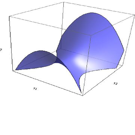
Figure 11: Examples of decision surfaces for linear Gaussian CWM (homoscedastic case).

As for the linear t-CWM, the first and the second term in (28) are, respectively:

$$\ln\frac{p(\mathbf{x}|\Omega_{1})}{p(\mathbf{x}|\Omega_{0})} =\ln\left[\frac{\Gamma((\nu_{1}+q)/2)\Gamma(\nu_{0}/2)}{\Gamma((\nu_{0}+q)/2)\Gamma(\nu_{1}/2)}\right]+\frac{1}{2}\ln\frac{|\mbox{\boldmath$\Sigma$}_{0}|}{|\mbox{\boldmath$\Sigma$}_{1}|}+$$

$$\quad+\frac{\nu_{0}+q}{2}\ln\{\nu_{0}+\delta(\mathbf{x},\mbox{\boldmath$\mu$}_{0};\mbox{\boldmath$\Sigma$}_{0})\}-\frac{\nu_{1}+q}{2}\ln\{\nu_{1}+\delta(\mathbf{x},\mbox{\boldmath$\mu$}_{1};\mbox{\boldmath$\Sigma$}_{1})\}\>$$

$$\ln\displaystyle{\frac{p(y|\mathbf{x},\Omega_{1})}{p(y|\mathbf{x},\Omega_{0})}} =\ln\left[\frac{\Gamma((\zeta_{1}+1)/2)\Gamma(\zeta_{0}/2)}{\Gamma((\zeta_{0}+1)/2)\Gamma(\zeta_{1}/2)}\right]+\ln\frac{\sigma_{\epsilon,0}}{\sigma_{\epsilon,1}}$$

$$\quad+\frac{\zeta_{0}+1}{2}\ln\left[\zeta_{0}+\left(\frac{(y-\mathbf{b}_{0}^{\prime}\mathbf{x}-b_{00}}{\sigma_{\epsilon,0}}\right)^{2}\right]-\frac{\zeta_{1}+1}{2}\ln\left[\zeta_{1}+\left(\frac{(y-\mathbf{b}_{1}^{\prime}\mathbf{x}-b_{10})}{\sigma_{\epsilon,1}}\right)^{2}\right]\>.$$

Then, equation (28) is satisfied for $(\mathbf{x},y)\in\mathbb{R}^{d+1}$ such that:

$$c(\nu_{0},\nu_{1},\zeta_{0},\zeta_{1})+\ln\frac{\sigma_{\epsilon,0}}{\sigma_{\epsilon,1}}+\frac{\zeta_{0}+1}{2}\ln\left[\zeta_{0}+\left(\frac{y-\mathbf{b}_{0}^{\prime}\mathbf{x}-b_{00}}{\sigma_{\epsilon,0}}\right)^{2}\right]+\\ -\frac{\zeta_{1}+1}{2}\ln\left[\zeta_{1}+\left(\frac{y-\mathbf{b}_{1}^{\prime}\mathbf{x}-b_{10}}{\sigma_{\epsilon,1}}\right)^{2}\right]+\frac{1}{2}\ln\frac{|\mbox{\boldmath$\Sigma$}_{0}|}{|\mbox{\boldmath$\Sigma$}_{1}|}\\ +\frac{\nu_{0}+q}{2}\ln\{\nu_{0}+\delta(\mathbf{x},\mbox{\boldmath$\mu$}_{0};\mbox{\boldmath$\Sigma$}_{0})\}-\frac{\nu_{1}+q}{2}\ln\{\nu_{1}+\delta(\mathbf{x},\mbox{\boldmath$\mu$}_{1};\mbox{\boldmath$\Sigma$}_{1})\}+\ln\frac{\pi_{1}}{\pi_{0}}=0\>,$$ (31)

where

$$c(\nu_{0},\nu_{1},\zeta_{0},\zeta_{1})=\ln\left[\frac{\Gamma((\zeta_{1}+1)/2)\Gamma(\zeta_{0}/2)}{\Gamma((\zeta_{0}+1)/2)\Gamma(\zeta_{1}/2)}\right]+\ln\left[\frac{\Gamma((\nu_{1}+q)/2)\Gamma(\nu_{0}/2)}{\Gamma((\nu_{0}+q)/2)\Gamma(\nu_{1}/2)}\right]\>.$$

We remark that, in this case, the decision surfaces are elliptical.

References

- (1)
- Anderson (1972) Anderson, J.A. (1972). Separate sample logistic discrimination, Biometrika, 59, 19-35.
- Anderson (1984) Anderson, T.W. (1984). An Introduction to Multivariate Statistical Analysis, John Wiley & Sons, New York, 2nd Edition.
- Andrews et al. (2002) Andrews, R.L., Ansari, A., Currim, I.S. (2002). Hierarchical Bayes versus finite mixture conjoint analysis models: a comparison of fit, prediction, and partworth recovery, Journal of Marketing, 39, 87-98.
- Bernardo and Girón (1992) Bernardo J.M, Girón F.J. (1992). Robust Sequential Prediction from non-random samples: the election night forecasting case. In: Bernardo J.M., Berger J.O., Dawid A.P., Smith A.F.M. (Eds.), Bayesian Statistics 5, Oxford University Press, 61-77.
- Campbell and Mahon (1974) Campbell N.A. and Mahon R.J. (1974). A multivariate study of variation in two species of rock crab of genus Letpograspus, Australian Journal of Zoology, 22, 417-455.
- Cerioli (2010) Cerioli, A. (2010). Multivariate Outlier Detection with high-breakdown estimators, Journal of the American Statistical Society, 105, n. 489, 147-156.
- Cuesta-Albertos et al. (2008) Cuesta-Albertos, J.A., Matrán, C., Mayo-Iscar, A. (2008). Trimming and likelihood: robust location and dispersion estimation in the elliptical model, The Annals of Statistics, 36, n.5, 2284-2318.
- De Sarbo and Cron (1988) De Sarbo W.S., Cron W.L. (1988). A maximum likelihood methodology for clusterwise linear regression, Journal of Classification, 5, 248-282.
- Dayton and Macready (1988) Dayton, C.M., Macready, G.B. (1988). Concomitant-Variable Latent-Class Models, Journal of the American Statistical Association, 83, 173-178.
- DeSarbo and Cron (1988) DeSarbo, W.S., Cron, W.R. (1988). A Conditional Mixture Maximum Likelihood Methodology for Clusterwise Linear Regression, Journal of Classification, 5, 249- 289.
- Dickey (1967) Dickey, J.T. (1967). Matricvariate Generalizations of the Multivariate t Distribution and the Inverted Multivariate t Distribution, The Annals of Mathematical Statistics, 38, 511-518.
- Engster and Parlitz (2006) Engster, D., Parlitz, U. (2006). Local and Cluster Weighted Modeling for Time Series Prediction. In: Schelter B., Winterhalder M., Timmer J. (Eds.), Handbook of Time Series Analysis. Recent theoretical developments and applications. Wiley, Weinheim, 39-65.
- Everitt and Hand (1981) Everitt, B.S., Hand D.J. (1981). Finite Mixture Distributions. Chapman & Hall, London.
- Faria and Soromenho (2010) Faria, S., Soromenho, G. (2010). Fitting mixtures of linear regressions, Journal of Statistical Computation and Simulation, 80, 201-225.
- Frühwirth-Schnatter (2005) Frühwirth-Schnatter, S. (2005). Finite Mixture and Markov Switching Models. Springer, Heidelberg.
- Gallegos and Ritter (2009) Gallegos M.T., Ritter G. (2009). Trimming algorithms for clustering contaminated grouped data and their robustness, Advances in Data Analysis and Classification, 3, 135-167.
- Gallegos and Ritter (2009b) Gallegos M.T., Ritter G. (2009b). Trimmed ML estimation of contaminated mixtures, Sankhya, 71-A, part 2, 164-220.
- Gershenfeld (1997) Gershenfeld, N. (1997). Non linear inference and Cluster-Weighted Modeling. Annals of the New York Academy of Sciences, 808, 18 -24.
- Gershenfeld et al. (1999) Gershenfeld, N., Schoner, B., Metois, E. (1999). Cluster-weighted modelling for time-series analysis. Nature, 397, 329-332.
- Gershenfeld (1999) Gershenfeld, N. (1999). The Nature of Mathematical Modelling. Cambridge University Press, Cambridge, 101-130.
- Greselin and Ingrassia (2010) Greselin, F., Ingrassia, S. (2010). Constrained monotone EM algorithms of multivariate distributions, Statistics & Computing, 20, 9-22.
- Greselin et al. (2011) Greselin F., Ingrassia S., Punzo A. (2011). Assessing the pattern of covariance matrices via an augmentation multiple testing procedure, Statistical Methods & Applications, 2011, to appear.
- Hurn et al. (2003) Hurn, M., Justel, A., Robert C.P. (2003). Estimating Mixtures of Regressions Journal of Computational and Graphical Statistics, 12, 55-79.
- Hurvich et al. (1998) Hurvich, C.M., Simonoff J.S., Tsai C.-L. (1998). Smoothing parameter selection in non parametric regression using an improved Akaike information criterion, Journal of the Royal Statistical Society B, 60, 271-294.
- Ingrassia (2004) Ingrassia S. (2004). A likelihood-based constrained algorithm for multivariate normal mixture models, Statistical Methods & Applications, 13, 151-166.
- Ingrassia and Rocci (2007) Ingrassia S. and Rocci R. (2007). Constrained monotone EM algorithms for finite mixture of multivariate Gaussians, Computational Statistics & Data Analysis, 51, 5339-5351.
- Jansen (1993) Jansen, R.C. (1993). Maximum likelihood in a generalized linear finite mixture model by using the EM algorithm, Biometrics, 49, 227-231.
- Jordan (1995) Jordan, M.I. (1995). Why the logistic function? A tutorial discussion on probabilities and neural networks, MIT Computational Cognitive Science Report 9503.
- Jordan and Jacobs (1994) Jordan, M.I., Jacobs, R.A. (1994). Hierarchical mixtures of experts and the EM algorithm. Neural Computation, 6, 181-224.
- Kan and Zhou (2006) Kan, R., Zhou, G. (2006). Modelling non-normality using multivariate t: Implications for asset pricing. Working paper. Washington University, St. Louis.
- Kotz and Nadarajah (2004) Kotz, S., Nadarajah, S. (2004), Multivariate Distributions and Their Applications, Cambridge University Press, New York.
- Lange et al. (1989) Lange, K.L., Little, R.J.A., Taylor, J.M.G. (1989). Robust Statistical Modeling Using the Distribution, Journal of the American Statistical Society, 84, n. 408, 881-896.
- Leisch (2004) Leisch, F. (2004). Flexmix: A general framework for finite mixture models and latent class regression in R. Journal of Statistical Software, 11(8), 1-18.
- Leisch (2008) Leisch, F. (2008). Modelling Background Noise in Finite Mixtures of Generalized Linear Regression Models, in “P. Brito (Ed.),Compstat 2008-Proceedings in Computational Statistics, Physica Verlag, Heidelberg, Germany, 385-396.
- Liesenfeld and Jung (2000) Liesenfeld, R., Jung, R.C. (2000). Stochastic volatility models: conditional normality versus heavy-tailed distributions, Journal of Applied Econometrics, 15, 137-160.
- Liu et al. (2004) Lin T.I., Lee J.C. and Ni H.F. (2004). Bayesian analysis of mixture modelling using the multivariate distribution, Statistics and Computing, 14, 119-130.
- Liu and Rubin (1995) Liu, C., Rubin D.M. (1995). ML Estimation of the Distribution using EM and its Extensions, ECM and ECME, Statistica Sinica, 5, 19-39.
- Mardia et al. (1979) Mardia, K.V., Kent, J.T., Bibby, J.M. (1979). Multivariate Analysis. Academic Press, London.
- McLachlan and Basford (1988) McLachlan, G.J., Basford, K.E. (1988). Mixture Models: Inference and Applications to Clustering. Marcel Dekker, New York.
- McLachlan and Peel (1998) McLachlan, G.J., Peel, D. (1998). Robust cluster analysis via mixtures of multivariate t-distributions. In: A. Amin, D. Dori, P. Pudil, and H. Freeman (Eds.), Lecture Notes in Computer Science, Vol. 1451. Springer-Verlag, Berlin, 658-666.
- McLachlan and Peel (2000) McLachlan, G.J., Peel, D. (2000). Finite Mixture Models. Wiley, New York.
- Nadarajah and Kotz (2005) Nadarajah, S., Kotz, S. (2005). Mathematical properties of the multivariate distributions, Acta Applicandae Mathematicae, 89, 53-84.
- Newcomb (1886) Newcomb, S. (1886). A generalized theory of the combination of observations so as to obtain the best result, American Journal of Mathematics, 8, 343-366.
- Ng and McLachlan (2007) Ng, S.K., McLachlan, G.J. (2007). Extension of mixture-of-experts networks for binary classification of hierarchical data, Artificial Intelligence in Medicine, 41, 57-67.
- Ng and McLachlan (2008) Ng, S.K., McLachlan, G.J. (2008). Expert networks with mixed continuous and categorical feature variables: a location modeling approach. In: H. Peters and M. Vogel (Eds.), Machine Learning Research Progress. Hauppauge, New York, 355-368.
- Nierenberg et al. (1989) Nierenberg D.W., Stukel T.A., Baron J., Dain B.J., Greenberg R. (1989). Determinants of plasma levels of beta-carotene and retinol, American Journal of Epidemiology, 130, n.3, 511-521.
- Pearson (1894) Pearson, K. (1894). Contributions to the mathematical theory of evolution, Philosophical Transactions of the Royal Society of London A, 185, 71-110.
- Peel and McLachlan (2000) Peel, D., McLachlan, G.J. (2000). Robust mixture modelling using the distribution, Statistics & Computing, 10, 339-348.
- Peng et al. (1996) Peng, F., Jacobs, R.A., Tanner, M.A. (1996). Bayesian inference in mixtures-of-experts and hierarchical mixtures-of-experts models with an application to speech recognition. Journal of the American Statistical Association, 91, 953-960.
- Pinheiro et al. (2001) Pinheiro J.C., Liu, C., Wu Y.N. (2001). Efficient algorithms for robust estimation in linear mixed-effects models using the multivariate distribution, Journal of Computational and Graphical Statistics, 10, 249-276.
- Quand (1972) Quandt R.E. (1972). A new approach to estimating switching regressions, Journal of the American Statistical Society, 67, 306-310.
- Riani et al. (2008) Riani, M., Cerioli, A., Atkinson, A.C., Perrotta, D., Torti F. (2008). Fitting mixtures of regression lines with the forward search, in ”Mining Massive Data Sets for Security, eds. F. Fogelman-Soulié, D. Perrotta, J. Piskorki and R. Steinberg”, IOS Press, Amsterdam, 271-286.
- Riani et al. (2009) Riani, M., Atkinson, A.C., Cerioli, A. (2009). Finding an unknown number of multivariate outliers, Journal of the Royal Statistical Society B, 71, n.2, 447-466.
- Schlattmann (2009) Schlattmann P. (2009). Medical Applications of Finite Mixture Models, Springer-Verlag, Berlin-Heidelberg.
- Schöner and Gershenfeld (2001) Schöner, B., Gershenfeld, N. (2001). Cluster Weighted Modeling: Probabilistic Time Series Prediction, Characterization, and Synthesis. In: Mees, A.I. (Ed.), Nonlinear Dynamics and Statistics. Birkhauser, Boston, 365-385.
- Schöner (2000) Schöner, B. (2000). Probabilistic Characterization and Synthesis of Complex Data Driven Systems, Ph.D. Thesis, MIT.
- Simonoff (2003) Simonoff, J.S. (2003). Analyzing Categorical Data. Springer, New York.
- Titterington et al. (1985) Titterington, D.M., Smith A.F.M., Makov, U.E. (1985). Statistical Analysis of Finite Mixture Distributions. Wiley, New York.
- Wang et al. (1996) Wang P., Puterman M.L., Cockburn I., Le N. (1996). Mixed Poisson regression models with covariate dependent rates, Biometrics, 52, 381-400.
- Wedel (2002) Wedel, M. (2002). Concomitant variables in finite mixture models. Statistica Nederlandica, 56, n.3, 362-375.
- Wedel and De Sarbo (1995) Wedel, M., De Sarbo W. (1995). A mixture likelihood approach for generalized linear models, Journal of Classification, 12, 21-55.
- Wedel and De Sarbo (2002) Wedel, M., De Sarbo W. (2002). Market segment derivation and profiling via a finite mixture model framework, Marketing Letters, 13, 17-25.
- Wedel and Kamakura (2000) Wedel, M., Kamakura, W.A. (2000). Market Segmentation. Conceptual and Methodological Foundations. Kluwer Academic Publishers, Boston.
- Zellner (1976) Zellner, A. (1976). Bayesian and Non-Bayesian Analysis of the Regression Model with Multivariate Student- Error Terms, Journal of the American Statistical Society, 71, 400-405.