A Layer Correlation Technique for Pion Energy Calibration at the 2004 ATLAS Combined Beam Test

Abstract

A new method for calibrating the hadron response of a segmented calorimeter is developed. It is based on a principal component analysis of the calorimeter layer energy deposits, exploiting longitudinal shower development information to improve the measured energy resolution. Corrections for invisible hadronic energy and energy lost in dead material in front of and between the ATLAS calorimeters were calculated with simulated Geant4 Monte Carlo events and used to reconstruct the energy of pions impinging on the calorimeters during the 2004 Barrel Combined Beam Test at the CERN H8 area. For pion beams with energies between 20 and 180 GeV, the particle energy is reconstructed within 3% and the energy resolution is improved by about 20% compared to the electromagnetic scale.

I Introduction

In general, the response of a calorimeter to hadrons will be lower than for particles which only interact electromagnetically, such as electrons and photons. This is due to energy lost in hadronic showers in forms not measurable as an ionization signal, i.e. nuclear break-up, spallation, and excitation, energy deposits arriving out of the sensitive time window (such as delayed photons), soft neutrons, and particles escaping the detector (Fig. 1). The shower has an electromagnetic and a hadronic component. The size of the former increases with energy, giving rise to a non-linear calorimeter response to impinging hadrons if the calorimeter response to the electromagnetic and hadronic parts of the shower is different. Such calorimeters are called non-compensating. Moreover, hadronic showers exhibit large even-by-event fluctuations, degrading the measured energy resolution [1].

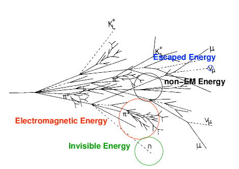
Figure 1: Components of a hadronic shower. Based on figure in [2].

The correlations between longitudinal energy deposits of the shower have been shown [3] to contain information on the electromagnetic and hadronic nature of the shower. This calibration method (called the Layer Correlation method in the following) aims to use such information to improve energy resolution and linearity. It is an alternative to the standard ATLAS hadronic calibration schemes.

II ATLAS and the 2004 Combined Beam Test

ATLAS [4] is one of the multi-purpose physics experiments at the CERN Large Hadron Collider (LHC) [5]. Physics goals include searching for the Higgs boson and looking for phenomena beyond the standard model of particle physics, such as supersymmetry. Many measurements to be performed by the LHC experiments rely on a correct reconstruction of hadronic final state particles.

In the central barrel region, the ATLAS calorimeters consist of the lead–-liquid argon (LAr) electromagnetic calorimeter and the steel-–scintillator Tile hadronic calorimeter. Both are intrinsically non-compensating.

The 2004 Combined Beam Test (Fig. 2) included a full slice of the ATLAS Barrel region, including the pixel detector, the silicon strip semiconductor tracker (SCT), the transition radiation tracker (TRT), the LAr and Tile calorimeters and the muon spectrometer. In addition, special beam-line detectors were installed to monitor the beam position and reject background events. Those include beam chambers monitoring the beam position and trigger scintillators. The pixel and SCT detectors were surrounded by a magnet capable of producing a field of 2 T, although no magnetic field was applied in the runs used for this study.

The calorimeters were placed so that the beam impact angle corresponded to a pseudorapidity of $\eta$ = 0.45 in the ATLAS detector. At this angle, the expected amount of material in front of the calorimeters is about 0.44 $\lambda_{I}$, where $\lambda_{I}$ is the nuclear interaction length. This includes the LAr presampler. The LAr calorimeter proper is longitudinally segmented in three layers that extend in total to 1.3 $\lambda_{I}$. The dead material between the Tile and LAr calorimeters spans about 0.6 $\lambda_{I}$. Finally the three longitudinal segments of the Tile calorimeter stretch in total for about 8.2 $\lambda_{I}$.

Events are selected by requiring signals in a trigger scintillator, beam chambers, and the inner detector compatible with one particle passing close to the nominal beam line. The TRT is used to reject positrons by making a cut on the detected transition radiation.

The positive pion beam is known to have a sizable proton contamination, which must be taken into account when deriving the calibration, since the calorimeter response for pions and protons is different. The fraction of protons in the beam was measured using the differing probabilities of pions and protons to emit transition radiation in the TRT. It was found to be 0% at a beam energy of 20 GeV, 45% at 50 GeV, 61% at 100 GeV, and 76% at 180 GeV.

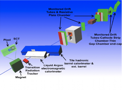
Figure 2: 2004 ATLAS Combined Beam Test set-up

III Method

The calibration scheme consists of compensation weights and dead material corrections. The former correct for the non-compensation of the calorimeters, while the latter compensate for energy lost in material with no calorimeter read-out.

$$E_{\textrm{corr}}^{\textrm{tot}}=E_{\textrm{tot}}^{\textrm{weighted}}+E_{\textrm{tot}}^{\textrm{DM}}$$ (1)

The dead material corrections (see below) have an inherent dependence on the beam energy. This dependence is removed by employing an iteration scheme, where at each step the final estimated energy of the former step is used, until the returned value is stable.

All corrections are extracted from a Geant4.7 [6, 7] Monte Carlo simulation, with an accurate description of the Combined Beam Test geometry. The QGSP_BERT physics list was used. The simulation gives access to both the true deposited energy in the detector material, as well as the signal read out from the calorimeters, including effects of the shaping electronics. The latter is calibrated at the electromagnetic scale, i.e. giving the correct deposited energy for electromagnetically showering particles, such as electrons and photons. The corrections are calculated using a Monte Carlo sample containing a scan of pion energies, from 15 to 230 GeV.

The energies of individual calorimeter cells are added up using a topological cluster algorithm [8]. The algorithm has three adjustable thresholds: Seed ($S$), Neighbor ($N$), and Boundary ($B$). First, seed cells having an energy above the $S$ threshold are found and a cluster is formed with this cell. Then, neighboring cells having an energy above the $N$ threshold are added to the cluster. This process is repeated until the cluster has no neighbors with an energy above the $N$ threshold. Finally, all neighboring cells having an energy above the $B$ threshold are added to the cluster. To avoid bias, the absolute values of the cell energies are used. The energy thresholds used for the $S$, $N$ and $B$ determination are set to, respectively, four, two, and zero times the expected noise in a given cell.

The reconstructed energy in a calorimeter layer $L$ is then obtained by considering all the topological clusters in the event and summing up the parts of the clusters that are part of that calorimeter layer.

III-A Eigenvectors of the covariance matrix

In total there are seven longitudinal calorimeter layers (the LAr presampler; the strips, middle, and back layers of the LAr calorimeter; and the A, BC, and D layers of the Tile calorimeter). The covariance matrix between these layers is calculated as

$$\textrm{Cov}(M,L)=\left<E_{M}^{\textrm{rec}}E_{L}^{\textrm{rec}}\right>-\left<E_{M}^{\textrm{rec}}\right>\left<E_{L}^{\textrm{rec}}\right>,$$ (2)

where $M$ and $L$ denote calorimeter layers and $E_{M}^{\textrm{rec}}$ is the energy reconstructed at the electromagnetic scale in calorimeter layer $M$.

An event can be regarded as a point in a seven-dimensional vector space of calorimeter layer energy deposits. Its coordinates can be expressed in a new basis of eigenvectors of the covariance matrix. These eigenvectors are ordered by decreasing eigenvalue, meaning that the projections along the first few eigenvectors contain most of the information on event-by-event longitudinal shower fluctuations. These projections are used as input to the calibration.

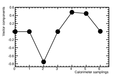
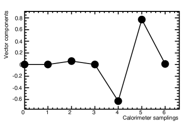
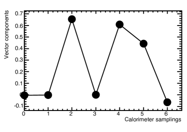
Figure 3: The first three eigenvectors of the covariance matrix in the basis of the original calorimeter layers.

Fig. 3 shows the first three eigenvectors of the covariance matrix in the basis of the original calorimeter layers.

We find that

$$E^{\textrm{rec}}_{\textrm{eig0}} \approx\frac{1}{\sqrt{6}}(-2E_{\textrm{LAr,middle}}+E_{\textrm{Tile,A}}+E_{\textrm{Tile,BC}}),$$

$$E^{\textrm{rec}}_{\textrm{eig1}} \approx\frac{1}{\sqrt{2}}(-E_{\textrm{Tile,A}}+E_{\textrm{Tile,BC}}),$$

$$E^{\textrm{rec}}_{\textrm{eig2}} \approx\frac{1}{\sqrt{3}}(E_{\textrm{LAr,middle}}+E_{\textrm{Tile,A}}+E_{\textrm{Tile,BC}}).$$

Thus, the zeroth eigenvector is essentially a difference between the Tile and LAr calorimeters, the first one a difference within the Tile calorimeter and the second one a sum of both calorimeters. The rest of the eigenvectors contain individual calorimeter layers.

III-B Compensation weights

The compensation weights account for the non-linear response of the calorimeters to hadrons. They are implemented as two-dimensional 128x128-bin lookup tables and are functions of the projections along the first two (zeroth and first) eigenvectors of the covariance matrix. Bi-linear interpolation is performed between the bins.

There is one weight table for each calorimeter layer, three for LAr and three for Tile. The LAr presampler is not weighted. Fig. 4 shows the weight table the first Tile layer. The total reconstructed energy is the sum of the weighted energies in each calorimeter layer.

$$E_{L}^{\textrm{weighted}} =w_{L}E_{L}^{\textrm{rec}}$$ (3)

$$E_{\textrm{tot}}^{\textrm{weighted}} =\sum_{L}E_{L}^{\textrm{weighted}}$$ (4)

Fig. 4 shows a weight table for the first layer of the Tile calorimeter.

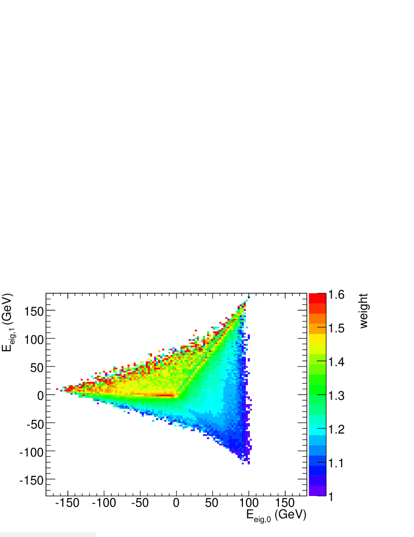
Figure 4: Compensation weights for the first Tile calorimeter layer.

III-C Dead material correction

Dead material is parts of the experiment that are neither active calorimeter read-out material (liquid argon or scintillator), nor sampling calorimeter absorbers (mostly lead or steel). Most of this material is in the LAr cryostat wall between the LAr and Tile calorimeters. There, pion showers are often fully developed, giving rise to large energy loss. To correct for these losses, the projections along the zeroth and second eigenvectors are used. When making the lookup table both the eigenvector projections and the dead material losses themselves are scaled with the true beam energy. Just as for the compensation weights, the table (Fig. 5) is two-dimensional with 128x128 bins and bi-linear interpolation is performed between the bins.

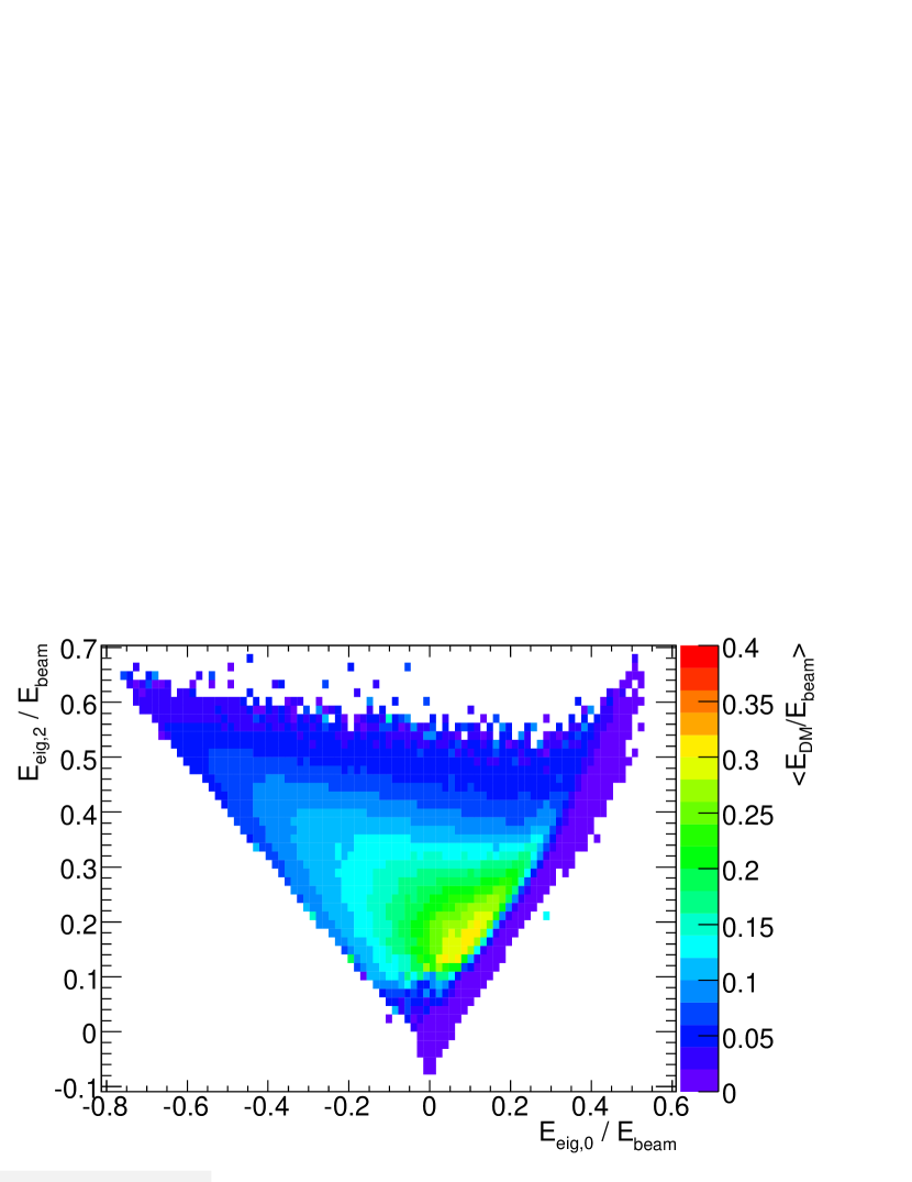
Figure 5: Lookup table for dead material correction.

In addition, there is also dead material before the LAr calorimeter (e.g. the inner detector) and leakage beyond the Tile calorimeter. These losses are small in comparison to those between the LAr and Tile calorimeters and were corrected for using a simple parameterization as a function of beam energy.

$$E^{\textrm{DM}}_{\textrm{other}}(E_{\textrm{beam}})=\left\{\begin{array}[]{rl}C_{1}+C_{2}\,\sqrt{E_{\textrm{beam}}}&\textrm{if }E_{\textrm{beam}}<E_{0}\\ C_{3}+C_{4}\,(E_{\textrm{beam}}-E_{0})&\textrm{otherwise,}\end{array}\right.$$ (5)

where $E_{0}=30000\ \mathrm{MeV}$. The resulting fitted parameters are

$$C_{1} =(-75\pm 31)\ \mathrm{MeV}$$ (6)

$$C_{2} =(5.78\pm 0.22)\ \sqrt{\mathrm{MeV}}$$ (7)

$$C_{3} =(931\pm 5)\ \mathrm{MeV}$$ (8)

$$C_{4} =0.01435\pm 0.0001$$ (9)

The final dead material correction is then the sum of these two contributions

$$E_{\textrm{tot}}^{\textrm{DM}}=E_{\textrm{LArTile}}^{\textrm{DM}}+E_{\textrm{other}}^{\textrm{DM}}$$ (10)

IV Method validation

Before applying it to beam test data, the calibration is validated on a Monte Carlo sample statistically independent of the one used for extracting the corrections. First, the performance of the compensation weights is evaluated, then the linearity and resolution of the method as a whole.

IV-A Compensation

The resulting reconstructed energy after applying compensation weights is compared to the true total deposited energy in the calorimeters as given by the Monte Carlo simulation. The event-by-event difference

$$E_{\textrm{tot}}^{weighted}-E_{\textrm{tot}}^{\textrm{true}}(\textrm{calo})$$ (11)

is considered. Fig. 6 shows the sample standard deviation of this variable as a function of beam energy. The performance of the Layer Correlation technique is compared to that of a simple calibration scheme where the energy of each event in the sample is multiplied by a single factor ($f_{\textrm{comp}}$) calculated to give the correct total deposited energy on average.

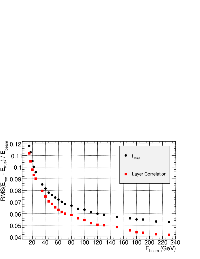
Figure 6: Sample standard deviation of the difference between the weighted calorimeter energy and the true deposited energy as given by the simulation, as a function of beam energy.

IV-B Linearity and resolution

The performance for the fully corrected energy reconstruction is assessed in terms of linearity (Fig. 7) and relative resolution (Fig. 8). The reconstructed energy distribution is fitted with a Gaussian function in an interval of two standard deviations on each side of the peak. This interval is found iteratively. Linearity and resolution are shown – first – at the electromagnetic scale – then – after successively applying the corrections: compensation weights, the LAr–Tile dead material correction, and finally after applying all corrections.

At the electromagnetic scale the calorimeter response is non-linear – as expected – and only about two thirds of the pion energy is measured. Weighting recovers about 80% to 90% of the incoming pion energy, while the LAr–Tile dead material correction accounts for an additional 8% to 10%. After all corrections the pion energy is correctly reconstructed within 1% for all beam energies. Each correction step makes the response more linear. The compensation weights give the most important contribution to linearity improvement at high energies, while the dead material effects play a more significant role at low energies.

The relative resolution improves when applying each additional correction step. At high beam energies (above 100 GeV) the contribution of the compensation weights to the improvement in energy resolution has the same magnitude as that of the LAr–Tile dead material corrections, while at lower energies the dead material corrections play a more important role.

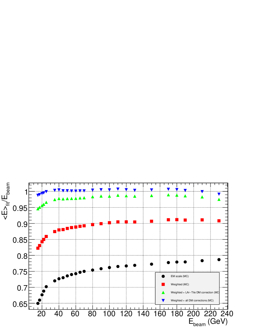
Figure 7: Linearity of reconstructed energy as a function of beam energy when successively applying the different parts of the correction. Monte Carlo simulation with pions only.

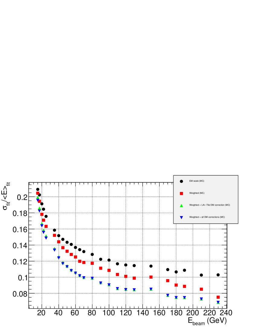
Figure 8: Resolution of reconstructed energy as a function of beam energy when successively applying the different parts of the correction. Monte Carlo simulation with pions only.

V Application to Beam Test Data

Finally, the method is applied to beam test data, which is compared with Monte Carlo samples with a weighted mixture of pions and protons to match the beam composition.

The linearity and relative resolution are shown in Fig. 9 and Fig. 10, respectively. Again, the reconstructed energy is fitted with a Gaussian function in an interval of two standard deviations on each side of the peak.

After all corrections, linearity is recovered within 2% for beam energies above 50 GeV (3% for 20 GeV).

The improvement in relative resolution when going from the electromagnetic scale to applying all corrections is about 17% to 22% in data and 17% to 29% in simulation. The relative resolution is smaller in Monte Carlo simulation than in data already at the electromagnetic scale, by about 8 to 18%, depending on beam energy. When applying the corrections, the ratio of the relative resolutions in data and simulation stays constant within 5%.

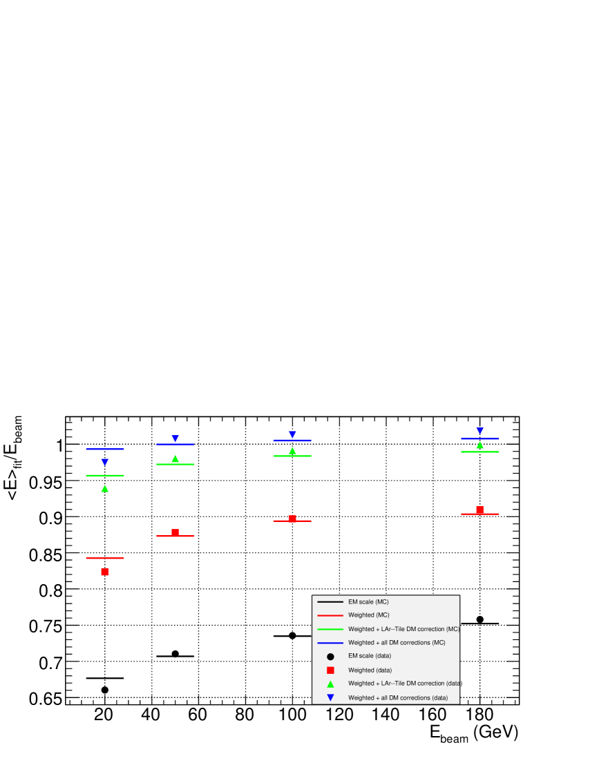
Figure 9: Linearity of reconstructed energy as a function of beam energy when successively applying the different parts of the correction. Data (markers) and Monte Carlo simulation (horizontal lines) are shown. Mixed beam of pions and protons.

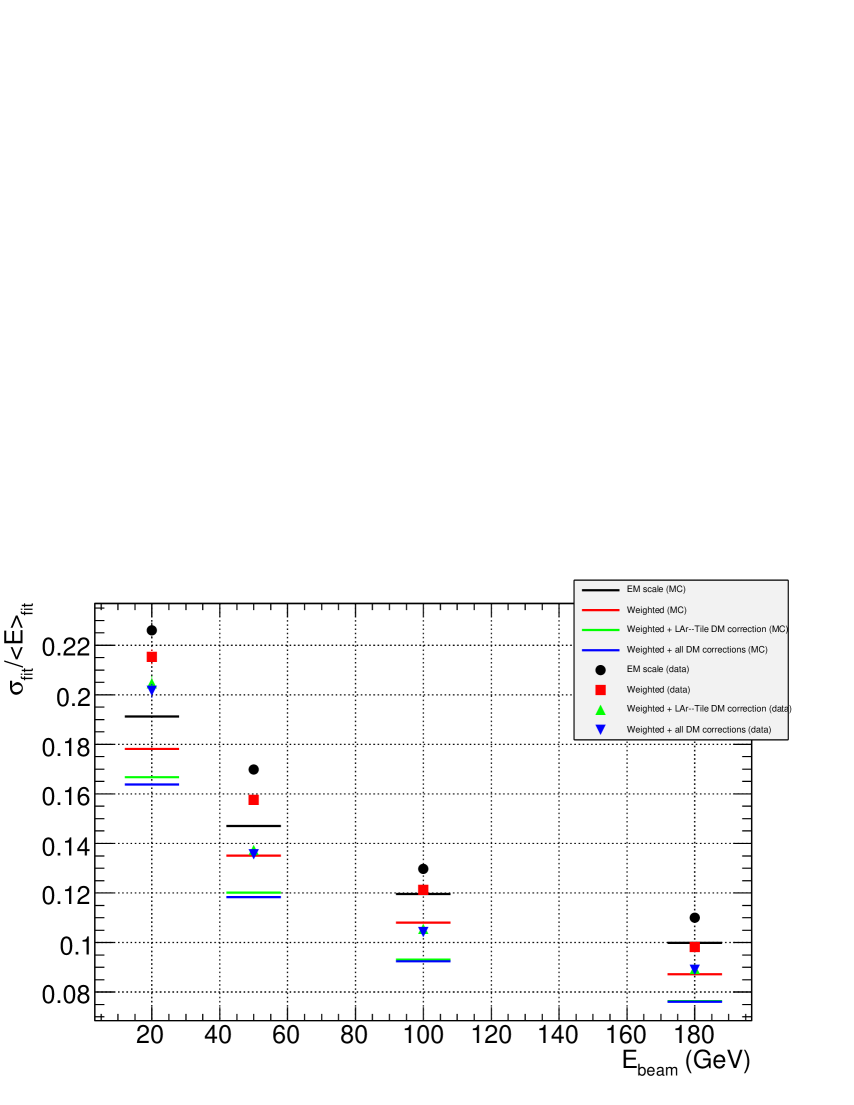
Figure 10: Resolution of reconstructed energy as a function of beam energy when successively applying the different parts of the correction. Data (markers) and Monte Carlo simulation (horizontal lines) are shown. Mixed beam of pions and protons.

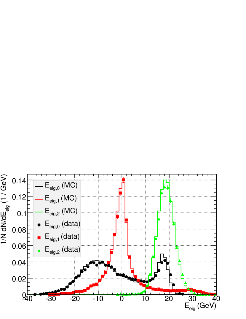
Figure 11: Distribution of the first three eigenvector projections in data and Monte Carlo simulation.

Fig. 11 shows the distribution of the first three eigenvector components for data and Monte Carlo simulation, with a beam of 50 GeV particles. Good agreement is obtained between data and simulation.

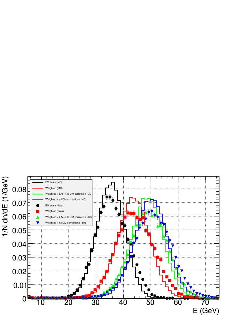
Figure 12: Distribution of reconstructed energy at the different correction steps in data and Monte Carlo simulation.

The shapes of the energy distributions for data and Monte Carlo simulation for 50 GeV particles are compared in Fig. 12. The distribution in the Monte Carlo simulation is narrower and less skewed than in the data. This is seen already at the electromagnetic scale. The effect is even larger at 20 GeV but less pronounced at higher energies.

VI Conclusions

The method was successfully applied to beam test data and is able to reconstruct the incoming pion energy within 3% in the energy range 20–180 GeV. Resolution is improved by about 20% compared to the electromagnetic scale.

The main deficiency of the Monte Carlo simulation is its inability to correctly describe the energy resolution in the beam test data. However, the relative improvement in resolution when applying the calibration is similar in data and Monte Carlo simulation.

References

- [1] R. Wigmans, Calorimetry – Energy Measurement in Particle Physics. Clarendon Press, Oxford, 2000.
- [2] C. Grupen and B. Shwartz, Particle Detectors, 2nd ed. Cambridge University Press, 2008.
- [3] N. Nakajima et al., “Correlation matrix method for Pb/Scint sampling calorimeter,” in Proceedings of the 2005 International Linear Collider Workshop, Mar. 2005.
- [4] G. Aad et al., “The ATLAS experiment at the CERN Large Hadron Collider,” J. Inst., vol. 3, no. 08, p. S08003, 2008.
- [5] L. Evans et al., “LHC machine,” J. Inst., vol. 3, no. 08, p. S08001, 2008.
- [6] S. Agostinelli et al., “Geant4: A simulation toolkit,” Nucl. Instrum. Meth. A, vol. 506, no. 3, pp. 250–303, 2003.
- [7] J. Allison et al., “Geant4 developments and applications,” IEEE Trans. Nucl. Sci., vol. 53, pp. 270–278, 2006.
- [8] W. Lampl et al., “Calorimeter clustering algorithms: Description and performance,” ATLAS Public Note ATL-LARG-PUB-2008-002, May 2008.