Non-parametric Deprojection of Surface Brightness Profiles of Galaxies in Generalised Geometries

Abstract

Aims. We present a new Bayesian non-parametric deprojection algorithm DOPING (Deprojection of Observed Photometry using and INverse Gambit), that is designed to extract 3-D luminosity density distributions $\rho$ from observed surface brightness maps $I$, in generalised geometries, while taking into account changes in intrinsic shape with radius, using a penalised likelihood approach and an MCMC optimiser.

Methods. We provide the most likely solution to the integral equation that represents deprojection of the measured $I$ to $\rho$. In order to keep the solution modular, we choose to express $\rho$ as a function of the line-of-sight (LOS) coordinate $z$. We calculate the extent of the system along the ${\bf z}$-axis, for a given point on the image that lies within an identified isophotal annulus. The extent along the LOS is binned and density is held a constant over each such $z$-bin. The code begins with a seed density and at the beginning of an iterative step, the trial $\rho$ is updated. Comparison of the projection of the current choice of $\rho$ and the observed $I$ defines the likelihood function (which is supplemented by Laplacian regularisation), the maximal region of which is sought by the optimiser (Metropolis Hastings).

Results. The algorithm is successfully tested on a set of test galaxies, the morphology of which ranges from an elliptical galaxy with varying eccentricity to an infinitesimally thin disk galaxy marked by an abruptly varying eccentricity profile. Applications are made to faint dwarf elliptical galaxy Ic 3019 and another dwarf elliptical that is characterised by a central spheroidal nuclear component superimposed upon a more extended flattened component. The result of deprojection of the X-ray image of cluster A1413 - assumed triaxial - the axial ratios and inclination of which are taken from the literature, is also presented.

1 Introduction

An integral step in the construction of dynamical models of galaxies is the recovery of the intrinsic luminosity density from the surface brightness that is observed projected on the plane of the sky (Magorrian et al. 1998; Kronawitter et al. 2000; Krajnovic et al. 2004). Such deprojection is non-trivial and indeed offers no unique solutions except for very specific configurations of geometry and inclination. As demonstrated by Rybicki (1987), the deprojection is degenerate for axisymmetric systems viewed at inclination angles, $i$, other than edge-on ($i=90$^∘). This is a consequence of the fact that the observed surface brightness cannot yield any information on a density term whose Fourier transform is non-zero only within a cone of half angle $90^{\circ}-i$ (the “cone of ignorance”). Gerhard & Binney (1996) report a family of analytical konus densities. Kochanek & Rybicki (1996) found a family of konus densities that have arbitrary densities in the equatorial plane. van den Bosch (1997) finds that konus densities contribute at most a few percent of the total galactic mass to the centre of elliptical galaxies with nuclear cusps, implying that their dynamical influence is minimal. Magorrian (1999) suggests that nearly face-on disk-like konus densities can be recognised via the unique signature they imprint on the line-of-sight (LOS) velocity profiles.

These problems notwithstanding, a great deal of effort has been put into the development of methodologies aimed at deprojecting two-dimensional photometric information. These include parametric formalisms designed by Palmer (1994), Bendinelli (1991) and Cappellari (2002), as well as non-parametric methods, such as the Richardson-Lucy Inversion scheme (Richardson 1972; Lucy 1974) and a method by Romanowsky & Kochanek (1997) (hereafter, RK).

The parametric methods work by making series expansions of the density (or brightness) and fit the brightness (or density) to the coefficient of the expansions; convergence is defined at a preset accuracy level. In Bendinelli (1991), the density is derived via a Gaussian expansion of the surface brightness profile, an idea further developed by Cappellari (2002). In Palmer (1994), the density is expanded in terms of angular polynomials and the projections of these are then fit to the surface brightness. These methods suffer from the basic drawback that the answer depends on the choice of the basis functions. Thus, the solution is forced to conform to a subset of all possible solutions. Even more worrisome is the fact that the validity of the goodness of fit measures, or “$\chi^{2}$ quantities” that are employed in these schemes to identify acceptable fits, is questionable, particularly in the presence of inhomogeneous noise (Bissantz & Munk 2001). On the whole, the fitting of non-linear functions, to what is usually noise-ridden incomplete data, over large dynamical ranges, is worrisome.

Deprojection of surface brightness profiles has also been attempted with the Abel integral equation, under the assumption of sphericity or axisymmetry with an edge-on inclination (Merritt, Meylan & Mayor 1997; Merritt & Tremblay 1993; Gebhardt et al. 1996).

An example of a non-parametric inversion scheme is the Richardson-Lucy algorithm (Richardson 1972; Lucy 1974), which has been widely used in the stellar dynamical context. It is a simple deprojection scheme that works by iterating toward increasingly better approximations to the density that fits the data. However, absolute convergence is not sought in this framework — rather, the iterations are stopped when the density is judged to be a good fit to the observations. In lieu of this imposed clause in the code, progressive iterations would produce increasingly more unphysical densities. This lack of a robust convergence criterion is cause for dissatisfaction with the Richardson Lucy scheme. Moreover, implementations of the same, within Astronomy, have not incorporated either radial variations of intrinsic shape or deviations from sphericity.

The shortcomings of Lucy’s algorithm are overcome by the analysis of RK in their incorporation of monotonicity and positivity into the sought solution and by their more satisfying convergence criterion. RK construct their density profile as a series of stacked blocks in the space of one quadrant of the meridional plane of their axisymmetric (by assumption) galaxy. The density values at radially adjacent locations are connected through linear interpolation. The summation of the projections of each of the density blocks along the LOS, give the surface brightness at a given location in the plane of the sky (where a brightness measurement is reported). This estimated brightness is then compared to the observed brightness; the algorithm attempts to minimise this statistic while imposing the smoothing condition through a bias function, thus providing a more satisfying convergence criterion than included in Lucy’s algorithm. However, this scheme too fails to allow for deprojection in general triaxial geometries; specifically, it is designed to reproduce axisymmetric systems. Moreover, the validity of interpolation, in systems where local gradients can be steep, is also worrisome.

Magorrian (1999) also advances a scheme similar to RK’s expect that he implements a penalty function in his definition of likelihood. The imposed penalty is achieves nearest-neighbour smoothing. The fundamental shortcomings of this scheme are the same as what plagues RK’s method. There is no apriori reason to belive that the galaxy under consideration is axisymmetric; triaxiality is a much more general model. Moreover, the requirement in this work, for density to behave like a power-law on local scales, implies that the method will fail in the presence of even moderate gradients in density; in this sense, the recovered answer could be sensitive to the binning details of the 2D grid on which the density structure is placed.

In this paper, we present a new, Bayesian non-parametric algorithm that implements an MCMC optimiser, in order to tackle the deprojection of observed photometry of galaxies. Completely free-form solutions for the 3D density are provided with the constraint of positivity imposed by hand. The scheme is a penalised likelihood procedure. We refer to this algorithm as DOPING - an acronym for Deprojection of Observed Photometry using an INverse Gambit. The algorithm is easy to implement and each run typically takes about a a couple of minutes on a state-of-the art personal computer.

The most distinguishing feature of DOPING is that it can tackle deprojection in virtually any geometry, as long as we can express the intrinsic shape parameters (such as eccentricities) in analytical relations with the projected shape parameters. DOPING can be applied to deproject surface brightness maps of elliptical as well as disk galaxies. This is possible, while taking intrinsic shape variation into account.

The first major application of this algorithm to galaxies (Chakrabarty $\&$ McCall, 2009) is the study of the deprojected luminosity profiles of 100 early type galaxies observed as part of the ACS Virgo Cluster Survey (Côté et al. 2004). As these systems do not exhibit significant variations in position angle, the preliminary version of DOPING that is presented here, considers position angle to be a constant. However the code can account for changes in position angle and the skeletal scheme for the inclusion of a radially varying position angle is presented later in §5.6.

The following section begins with a discussion of the broad framework of our algorithm DOPING, a moves to an exposition of the technical details of the code in §2. In §3, we talk about the application of DOPING to a test case and corroborate the robustness of the algorithm. Application to the real ACS photometry of the galaxy vcc9 is also discussed in §4. §3 explores the effects of varying ambient conditions such as inclination and the assumed geometry. §5 is devoted to discussions and conclusions that are to be drawn from the work. In the appendix, a discussion of the details of various aspects of DOPING is presented.

2 Overview of the Algorithm

DOPING is a code designed to perform 3-D modelling of systems, given 2-D images, in a variety of spatial geometries. We iterate over trial 3-D luminosity density structures till the best match between the projection of the same and the measured 2-D surface brightness is obtained. Since deprojection is non-unique unless the intrinsic spatial geometry of the system is pinned down, we begin this section with a discussion on the motivation and details of how the detailed description of the geometry is achieved.

In particular, the true shape and inclination of a system can be deciphered, using DOPING, if:

• the system has a regular geometry, (by which we imply that it bears an $m$-fold symmetry) and

• the relative extent of the system along any three mutually orthogonal axes are known

or if

• the inclination to the LOS can be varied and the system viewed at multiple inclinations, in which case

• DOPING can perform in any geometry.

Below, we emphasise on deprojection given unknown inclination and in the triaxial geometry - the most relevant scenario for astrophysical systems.

In fact, for galaxy clusters, when SZe measurements are available, it is possible to measure the extent along all three observer coordinate-axes (two axes on the plane of the image and a third along the LOS), under the assumption that one photometric axis is coincident with a principle axis of the system. Thus, the true intrinsic shape and orientation of galaxy clusters can be predicted by inverting the X-ray surface brightness map at benchmark deprojection geometries (Chakrabarty, de Filippis $\&$ Russell 2008). Thus, the luminosity density of galaxy clusters can be uniquely determined. An example of this is discussed in § refsec:A1413.

However, for triaxial galaxies, the LOS extent is unknown; thus, for galaxies, the true 3-D shape and orientation cannot be deciphered. Therefore, for galaxies, we need to assume values for the polar inclination and the missing axial ratio. The recovery of the 3-D luminosity density is undertaken, given these assumptions. Also, in this work, we hold the azimuthal inclination zero.

It merits mention that our assumptions are not over-indulgent. Any deprojection invokes assumptions about the intrinsic geometry and the inclinations of the system. Thus, when axisymmetry is assumed, it implies that one of the intrinsic axial ratios is held as unity, the polar inclination is also assumed and the azimuthal inclination is set to zero. This is similar to DOPING in that the user needs to assume one inclination and one intrinsic axial ratio for galaxies. However, when greater observational information is available, as for galaxy clusters, DOPING does not need to invoke any assumptions, in contrary to axisymmetry-assuming algorithms.

The assumptions are designed to be given as inputs for a given run of DOPING (Section 2.1 to 2.10). Given that each run of DOPING takes about 2 minutes on a 3.2GHz CPU processor , it is possible to scan over a wide range of inclination and axial ratio values to record a range of corresponding 3-D density distributions. The justification of assumptions is discussed in details in §5.5 and 5.3.

In order to design a recursive algorithm that can perform deprojection in varied geometries, the trial 3-D density structure should preferably not be treated as function of a coordinate that characterises the geometry at hand. Instead, we need to express the 3-D density as function of generic coordinates. However, a mapping between such generic coordinates and the system geometry is then required. This is what we aim for (§ 2.5). In fact, we express this mapping by calculating the extent of the system along the LOS, through any given point on the image. Such a calculation invokes values of all available shape and size related parameters - this is discussed in § 2.5.

Once this is established, we then discuss (§ 2.11) details of how to iterate towards the best possible 3-D density structure that projects to the observed surface brightness map.

2.1 Coordinates used

In any kind of deprojection problem, the two coordinate systems that suggest themselves readily are the body coordinate frame ($X,Y,Z$) and the observer’s coordinate frame ($x,y,z$). Here the three principal axes of the ellipsoidal system are considered to be along the $\hat{\bf X},\hat{\bf Y}\>\&\>\hat{\bf Z}$ vectors. The LOS coordinate is $z$ while the plane of the image is considered scanned by the $x-y$ coordinates, i.e the image plane is given by the equation $z$=0. The $Z$-axis is considered to be at an inclination angle $i$ relative to the line-of-sight, i.e. the $z-$axis.

The $X,Y,Z$ and $x,y,z$ coordinate systems will be related by two consecutive rotations. For triaxial galaxies, neither of these rotational angles is an observable in general. Only when the galaxy is highly flattened, can the inclination of its rotational axis to the LOS be estimated. The general lack of information about inclinations in triaxial systems will need to be compensated for by assumptions - while the assumed value of one inclination angle is provided as an input to the algorithm, the choice of the other inclination angle in this unconstrained situation is chosen to be such that our calculations are rendered easy: we assume that one of the principle axes lies entirely in the plane of the image. In fact, we choose this to be the $X$-axis. Then, the $X$-axis is also a photometric axis. We align our observer coordinate system such that the $x$-axis lies along the $X$-axis, i.e. $\hat{\bf X}=\hat{\bf x}$. Then, $\hat{\bf x}$ is along the photometric major axis for an oblate system but along the photometric minor axis in case of a prolate system. If the system in hand is triaxial, then there exists a scope for a degeneracy, depending on whether the $x$-axis is considered the major or minor axis. When the input for the assumed value of one inclination is $i$, the equations relating the ($X,Y,Z$) system of coordinates to the ($x,y,z$) system are:

$$X = x$$ (1)

$$Y = y\cos{i}+z\sin{i}$$

$$Z = -y\sin{i}+z\cos{i}.$$

Thus, all 3-D density distributions that are recovered by DOPING are obtained under the assumption that the azimuthal inclination is zero. The algorithm can in principle, also work for a choice of non-zero azimuthal inclinations; a range of 3-D density distributions for a range of choices of this angle is achievable. However, in lieu of measured information, the specification of such a range is impossible. This is discussed in detail in §5.3.

2.2 Input Data

The image or the projection of the galaxy on the plane of the sky is treated as built of concentric isophotes. Let the image be built of $N_{data}$ number of isophotes and the isophotal annulus between the $k-1^{th}$ and $k^{th}$ isophotes be the $k^{th}$ isophotal annulus. Here, $k=1,\ldots,N_{data}$.

The observables that DOPING processes are the characteristics of the isophotes, namely, the surface brightness measurement and the shape parameters of a given isophote, along with the value of its extent along the photometric $x$-axis, i.e. in effect, the surface brightness map of the galaxy. Several routines are available for the production of such a data set; such as the IRAF implementation of the task ELLIPSE (Jedrzejewski, Davies $\&$ Illingworth 1987).

If the isophotal shape characteristics vary over the extent of the image, then it is possible to flag their values according to the isophotal annulus that they are observed in; thus, the projected axial ratio in the $k^{th}$ isophotal annulus is $q_{pk}$ and the semi-$x$ axis extent of the $k^{th}$ isophote is $a_{k}$. Thus, the input data table in our work presents: an index for the isophotal annulus or $k$, the semi-$x$ axis $a_{k}$, projected axial ratio $q_{pk}$ and brightness values $I_{obs}^{k}$, for each $k$ i.e. each isophotal annulus that the image is binned into. Now, the isophotes of elliptical galaxies are often seen to deviate from pure ellipses (e.g. Bender et al. 1988; van den Bosch et al. 1994; Ferrarese et al. 2006). Hence, the boxiness/diskiness parameters can also be included in the table. To keep the introduction of the algorithm simple, in the following discussion, we ignore the contribution of these deviations from the purely elliptical shape, knowing that these effects can be included easily into the isophotal equation as suggested by Jedrzejewski (1987). Even more severe deviations from the elliptical isophotal shape can be accommodated and these cases (that do not bear a strong relevance in astrophysics) are discussed later in §5.1. The representation of isophotes within DOPING is further discussed in AppendixA.

In the applications of the code discussed in this paper, the position angle of the isophotal semi-major axis is assumed constant, though scope exists within the algorithm to relax this. The overall scheme for such a relaxation is discussed later in §5.6 though the incorporation of the same being non-trivial, this will be presented within DOPING in a future contribution.

2.3 Bayesian Formulation

We seek the 3D luminosity density $\rho$ of the system, given the surface brightness (surface brightness) maps as the input measurements. The probability of spotting the density $\rho$, given the measurements, and all our background knowledge (assumptions) about the system ($K$) is:

$$\Pr(\rho|{SB},K)\propto\Pr(SB|\rho,K)\times{\Pr}(\rho|{K}).$$ (2)

This is the Bayesian statement of the problem. The first term on the right side of the proportional sign is the likelihood while the second term is the prior.

In general, the prior that we can use is a uniform one:

$$\Pr(\rho(\cdot)|{K}) = 1\quad{\rm{if}\>\rho(\cdot)>=0}$$ (3)

$$= 0\quad{\rm{otherwise}},$$

by which we imply that the prior probability is unity only if $\rho(x,y,z)$ is non-negative everywhere.

However, it is possible that for disk galaxies, $i$ can be established from observations. Thus, if the inclination is given as: $i=i_{0}\pm\delta$, then assuming Gaussian errors, our prior will have an additional factor that is proportional to $\exp[-(i-i_{0})^{2}/(2\delta^{2})]$.

2.4 Methodology

A prescribed system geometry would imply that the coordinates $x$, $y$ and $z$ are related in terms of the shape parameters, i.e. $z$ can be expressed in terms of $x$ and $y$. For example, under the assumption of triaxiality, an analytical relation links the $x$ and $y$ to the $z$ as $x,y,z$ is a point on the surface of a homeoid; this relation takes into account the local values of the inclinations and intrinsic axial ratios of the system.

We attempt to express the 3-D density at a point as function of the coordinates on the image plane (i.e. $x$ and $y$) and the LOS coordinate ($z$) for that point. However, As $x$ and $y$ are coordinates on the image plane, they can be measured while $z$ can be calculated for a given $x$-$y$ pair, from the aforementioned relation between $x$, $y$ and $z$. Once $z$ is established, a trial 3-D density can be integrated along the LOS, over this established range of $z$ values, and the projection compared to the value of surface brightness observed at the point $(x,y,0)$. However, for the aforementioned relation to be completely specified, the system geometry needs to be invoked. Here we describe how such a relation is specified in the astrophysical context.

For the deprojection of galactic surface brightness maps, if the galaxy is considered a single-component system, we assume the galaxy to be a triaxial ellipsoid. For multi-component galaxies, such as systems with a central component superimposed on an extended disky component, each component is typically ascribed a triaxial ellipsoidal geometry (Chakrabarty $\&$ McCall, in preparation). Isolated off-centred clumps can also be included in the modelling (see §4.3).

When the galaxy is modelled as triaxial, the details of system geometry are described in AppendixB. The crux of the matter is that to compensate for our ignorance about the two inclinations and one of the two projected axial ratios ($q_{p}$ and $q_{LOS}$) of an observed galaxy, we assume a value for one inclination $i$, set the other inclination (angle between ${\bf{X}}$ and ${\bf{x}}$-axis) to zero, assume a value for one intrinsic axial ratio $q_{1}$ and calculate the other intrinsic axial ratio $q_{2}$ from the relation that connects $q_{2}$ to $q_{1}$, $q_{p}$ and $i$. The assumptions made to facilitate deprojection under triaxiality are similar in number with those made when deprojection under axisymmetry is performed (see §2 and §5.5), although, for deprojection of galaxy clusters, DOPING does not need to make such assumptions (Chakrabarty, de Filippis $\&$ Russell 2008). Importantly, the range of 3-D luminosity density distributions recovered for various assumptions, can be gauged with DOPING.

The axial ratios mentioned above can all vary with distance away from system centre. Thus, the assumed axial ratio ($q_{1}$) can be described as any real function of $x$ (as long as the function is non-singular over the range covered in the measurements).

2.5 Mapping the LOS extent to the system geometry

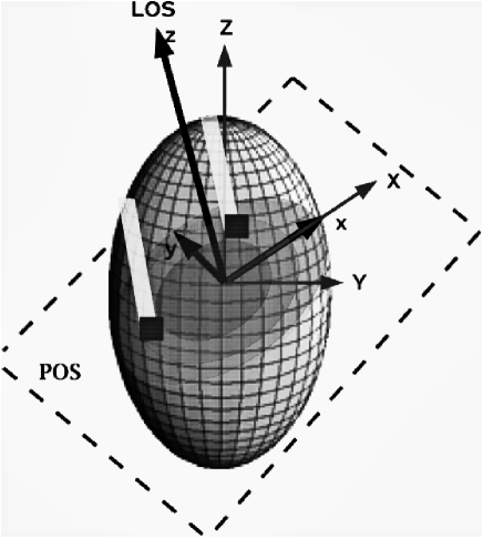
Figure 1: Figure showing geometrical considerations adopted in the design of the algorithm. The system is represented as the ellipsoid. The $X$, $Y$ and $Z$ axes (in thin black lines) represent the three principle axes of the system while $x$ and $y$ mark the photometric axes and the $z$-axis is the LOS (in thicker black lines). A rectangular section of the image plane (i.e. the $z$=0 plane) is represented by the tilted rectangle in the broken lines; this plane cuts the ellipsoid in an elliptical disk which is depicted by the translucent gray disk. Generic isophotal annuli on this disk are depicted in centrally increasing gray-scale intensity. Two generic points, lying inside the intermediate isophotal annulus, are shown as the two black squares. The extent of the system along the positive $z$-axis, at these two marked points are represented by the lengths of the white rectangles that are oriented parallel to the LOS. In the text, one such point, generically considered to be inside the $k^{th}$ isophotal annulus, is referred to as $(x_{j}^{k},y_{j}^{k},0)$, while the tip of the white rectangle emanating from this point is ascribed coordinates $(x_{j}^{k},y_{j}^{k},z_{max}^{jk})$. The extent along the negative $z$-axis is not shown in this diagram. The ellipsoidal shell that passes through $(x_{j}^{k},y_{j}^{k},z_{max}^{jk})$ is fully constrained (see § 2.5). Using $x_{j}^{k}$ and $y_{j}^{k}$, (coordinates of the known point on the image plane), the intrinsic shape parameters of the $k^{th}$ isophotal annulus ($a_{k}$, $q_{1k}$, $q_{2k}$) and the inclination $i$, the equation of this ellipsoid is solved to obtain the value of $z_{max}^{jk}$ (and $z_{min}^{jk}$). Thus, the $z$-extent through which a trial 3-D $\rho(x_{j}^{k},y_{j}^{k},z)$ has to be projected, is ascertained, for all $j$ and $k$.

As said before, our aimed deprojection requires evaluation of the characteristic extent along the $z$-axis of a point on the image plane. To accomplish this, we need to remind ourselves of all the relevant image characteristics of the given point on the image plane; this includes the surface brightness at this point, the local value of projected axial ratio at this point, etc. The determination of the $z$-height of a point on the image plane is discussed below and graphically represented in Figure 1.

We put the system on a regular 3-D Cartesian $x-y-z$ grid. We flag grid points that lie on the image i.e. the $z$=0 plane, according to the isophotal annulus that they lie in. We refer to the $j^{th}$ point inside the $k^{th}$ isophotal annulus as $(x_{j}^{k},y_{j}^{k},0)$. Here $j=1,\ldots,N_{k}$, where $N_{k}$ is the number of grid points with $z$=0, inside the $k^{th}$ isophotal annulus.

Through the point $(x_{j}^{k},y_{j}^{k},0)$, let the system extend along the $z$-axis, (i.e. the LOS), from $(x_{j}^{k},y_{j}^{k},z_{max}^{jk})$ to $(x_{j}^{k},y_{j}^{k},z_{min}^{jk})$. To determine $z_{max}^{jk}$ and $z_{min}^{jk}$, we pass a thin triaxial ellipsoidal shell through $(x_{j}^{k},y_{j}^{k},z_{max}^{jk})$ and $(x_{j}^{k},y_{j}^{k},z_{min}^{jk})$. This ellipsoidal shell

1. is centred at (0,0,0),

2. projects at the assumed inclination $i$, to the $k^{th}$ elliptical annulus on the image, which in turn has an axial ratio of $q_{pk}$ and semi-axis $a_{k}$ along $\hat{\bf x}$.

3. has intrinsic axial ratios $q_{1k}$ and $q_{2k}$.

4. has the points $(x_{j}^{k},y_{j}^{k},z_{max}^{jk})$ and $(x_{j}^{k},y_{j}^{k},z_{min}^{jk})$ on it, of which the $x$ and $y$ coordinates are known grid points but $z_{max}^{jk}$ and $z_{min}^{jk}$ are undetermined.

Thus, if we can write the equation of this ellipsoid with $x=x_{j}^{k}$, $y=y_{j}^{k}$ and solve the equation for $z$, the resulting solutions for $z$ will be $z_{max}^{jk}$ and $z_{min}^{jk}$. (Since the equation of an ellipsoid is quadratic in $z$, there will be two solutions for $z$). To write the equation of the ellipsoid however, we need to know

• its extent along a principal axis - the extent along the $x$-axis, i.e. $X$-axis is known (=$a_{k}$).

• the angle between the $Z$-axis and the LOS - $i$ is known by assumption.

• its intrinsic axial ratios $q_{1k}$ and $q_{2k}$. In the absence of measured $q_{LOS}$, $q_{1k}$ is known by assumption. $q_{2k}$ is derived as follows.

$q_{pk}$ is related to $q_{1k}$ and $q_{2k}$ through a simple geometrical relation that also involves $i$:

$${q_{pk}^{2}}=\displaystyle{\frac{{q_{1k}^{2}}q_{2k}^{2}}{q_{1k}^{2}\cos^{2}(i)+q_{2k}^{2}\sin^{2}(i)}}.$$ (4)

This relation gives $q_{2}^{k}$ (see Chakrabarty, de Filippis $\&$ Russell 2008). In this way, we constrain all parameters that define the ellipsoidal shell that passes through the points $(x_{j}^{k},y_{j}^{k},z_{max}^{jk})$ and $(x_{j}^{k},y_{j}^{k},z_{min}^{jk})$ (points I to IV of first list in this subsection). The equation of such a fully characterised ellipsoid is

$$\displaystyle{(x_{k}^{j})^{2}+(y_{k}^{j})^{2}\displaystyle{({q_{2k}^{2}}{\cos{{}^{2}}{i}}+{q_{1k}^{2}}{\sin{{}^{2}}{i}})}+}$$

$$\displaystyle{z^{2}\displaystyle{({q_{2k}^{2}}{\sin{{}^{2}}{i}}+{q_{1k}^{2}}{\cos{{}^{2}}{i}})}-y_{k}^{j}z\sin{2i}\displaystyle{({q_{1k}^{2}}-{q_{2k}^{2}})}} = a_{k}^{2}.$$ (5)

Here $q_{1}^{k},q_{2}^{k},a_{k}$ and $i$ are all known. $x_{k}^{j}$ and $y_{k}^{j}$ are known since the point $x_{k}^{j},y_{k}^{j},0$ has been identified to lie inside the $k^{th}$ isophotal annulus. Thus, this quadratic equation is solved for $z$ and its two solutions are $z_{max}^{jk}$ and $z_{min}^{jk}$.

In this way, the extent of the system, along the $z$-axis, through any point on the 2-D image is determined. A schematic of this procedure is presented in Figure 1. We now continue with the nomenclature introduced in this section, to describe generic points lying inside generic isophotal annuli.

2.6 $z-histogram$s

In order to keep the formalism flexible, we seek a form of the 3-D density in terms of $z$.

Thus, we discretise the density structure $\rho(x_{j}^{k},y_{j}^{k},z)$ where $z\in[z_{min}^{jk},z_{max}^{jk}]$, $\forall\>j,k$. Actually, in our work, we bin the range $[0,z_{max}^{jk}]$, and find the luminosity density $\rho(\cdot)$ for only one half of the system (at positive $z$ only). The density for the other half is given using the symmetry argument $\rho(x,y,z)=\rho(-x,-y,-z)$, which is valid under the assumption of triaxial geometry. In other words, we invert the projection integral $I(x_{k}^{j},y_{k}^{j})=2\int_{0}^{z_{max}}\rho(x_{k}^{j},y_{k}^{j},z)dz$ instead of $I(x_{k}^{j},y_{k}^{j})=\int_{z_{min}}^{z_{max}}\rho(x_{k}^{j},y_{k}^{j},z)dz$.

We do this by binning the $z$-range between $z_{min}^{jk}$ and $z_{max}^{jk}$. The binning is logarithmic since the measurements of surface brightness values are typically obtained for an astronomical system at increasingly wider isophotal annuli. $\rho(x_{j}^{k},y_{j}^{k},z)$ is held a constant over each $z$-bin. Thus, the density structure along the $z$-axis, through the point $(x_{j}^{k},y_{j}^{k},0)$ on the image, looks like a 1-D histogram. We refer to this construction as the ${\bf{z-histogram}}$, corresponding to the point $(x_{j}^{k},y_{j}^{k},0)$. The $z$-range of a ${\bf{z-histogram}}$ spans the interval: $z_{min}^{jk}$ and $z_{max}^{jk}$. Thus, this $z$-range depends on the point on the image through which the ${\bf{z-histogram}}$ is constructed.

2.7 Why $z-histogram$s instead of $\xi-histograms$s

We choose the basis of $\rho$ to be $z$ instead of a function of the system shape such as the ellipsoidal radius $\xi$. Reliance of the deprojection of the observed surface brightness map on the intrinsic shape would curb the reach of the algorithm in the following two ways:

• systems with different geometries that cannot be ascribed a general triaxial shape cannot then be tracked by the same code. An example of such a system within the astrophysical context could be a galaxy that is better described by a cylindrical intrinsic shape, such as the LMC. surface brightness of such a galaxy can however be deprojected under the flexible DOPING, with minimal changes imposed on the algorithm. In this non-triaxial geometry, the calculation of the intrinsic axial ratios from the measured projected axial ratios (and hence the calculation of the $z$-height of any point on the image) is different from the triaxial case; these calculations are performed within a modular sub-routine, before the iterations begin. The rest of the algorithm (iterative search for the most likely density structure) is unaffected by the difference in the system geometry. Thus, the same code can be used to undertake deprojection in general geometries.

• luminosity density distributions of systems with imposed substructure or extra galactic components that are imposed on the background galactic structure (such as disk+bulge systems) cannot be obtained in a single-step, integrated fashion if the algorithm is designed exclusively within the geometry of the background structure.

However, it may be argued that the choice of $z$ as the basis function for $\rho$ will subvert the underlying geometry under which we deproject and the independent updating of the ${\bf{z-histograms}}$ will render the resulting density structure noisy. This is not the case. The system geometry is reinforced via:

• the determination of the $z$-height of a given point on the image plane. This value robustly reflects the intrinsic geometry of deprojection.

• penalising all solutions for $\rho$ that do not adhere to a form in which there is maximum variance between densities that are at different ellipsoidal radii but minimum variance between densities at the same $\xi$. This characteristic can be incorporated by introducing a penalty function that is proportional to the Laplacian of the current choice of $\rho$, where the Laplacian operator involves differentiation w.r.t. $\xi$. This is discussed in detail in the following subsection.

2.8 Laplacian regularisation

We understand that the sought solution for $\rho(x,y,z)$, as given by the assembly of $z$-histograms, is in need of regularisation. We choose to introduce this regularisation such that we achieve low-dimensional representation of higher-dimensional information. In particular, we are interested to recover density that is a function of $\xi$, i.e. we work with a penalty function that reflects the intrinsic geometric structure of the input space (Haykin 2008; Wang 2006).

Such sought, similarity based smoothing is ensured by adopting a penalty function ${\cal{P}}$ that is given in terms of the Laplacian of the object function:

$${\cal{P}} = \alpha\displaystyle{(\nabla^{2}\rho)^{2}}\quad{\textrm{where}}$$

$$\nabla^{2} \equiv \displaystyle{\frac{\partial^{2}}{\partial^{2}\xi}}$$ (6)

Here $\alpha>0$ is a regularisation parameter, that reflects a trade-off between maximising variance between $\rho$ at different $\xi$ and reinforcing the relevant deprojection geometry.

2.9 Density structure

DOPING works recursively, via an inverse approach. At every iterative step, a trial $\bf{z-histogram}$ is chosen for each grid point on the image, i.e. for a given $j$, $k$. Each such $\bf{z-histogram}$ is updated independently during an iterative step, to render the whole 3-D density structure of the galaxy updated. Such updating of the $\bf{z-histogram}$ is done while maintaining positivity of $\rho$.

Once updated, the density structure is projected on the $z$=0 plane and this projection is compared to the surface brightness data. This comparison defines the likelihood function which is maximised for the best match. The likelihood is supplemented with a penalty that was discussed in the last paragraph. The global maxima of the likelihood function is sought by our MCMC algorithm to yield the most likely density structure, given the surface brightness data. However, we choose only those solutions which are “smooth”, as dictated by the used regularisation scheme.

2.10 Likelihood

The probability of the data given the model - i.e. the observed surface brightness map, given a trial 3-D density - is expected to be normal. This is reinforced on the basis of the following.

The likelihood or the probability of a measured surface brightness map, given a choice of the 3-D density structure, has to be a function of the distance between the projection of the 3-D density on the image plane and the measured surface brightness. In particular, $\Pr(data|\rho(\cdot))$, is such that when the projection of $\rho(\cdot)$ on the image plane is concurrent with the measured surface brightness distribution, $\Pr(data|\rho(\cdot))$=1. Additionally, the further is $\int\rho(x_{k}^{j},y_{k}^{j},z)dz$ from the surface brightness measurement $I_{obs}^{k}$ in the $k^{th}$ isophotal annulus, the smaller is the likelihood; in fact, for $|\int\rho(x_{k}^{j},y_{k}^{j},z)dz-I_{obs}^{k}|\longrightarrow\infty$, $\Pr(data|\rho(\cdot))$=0. Since the likelihood is a function of the absolute distance between $\int\rho(x_{k}^{j},y_{k}^{j},z)dz$ and $I_{obs}^{k}$, (for any $k$), for two different 3-D densities $\rho_{1}(x_{K}^{j},y_{k}^{j},z)$ and $\rho_{2}(x_{K}^{j},y_{k}^{j},z)$, if $|\int\rho_{1}(x_{k}^{j},y_{k}^{j},z)dz-I_{obs}^{k}|=|\int\rho_{2}(x_{k}^{j},y_{k}^{j},z)dz-I_{obs}^{k}|$, it implies that $\Pr(I_{obs}^{k}|\rho_{1}(\cdot))=\Pr(I_{obs}^{k}|\rho_{2}(\cdot))$, i.e. the likelihood is symmetric about $I_{obs}^{k}\>\forall\>k$. Also, for two different surface brightness measurements, $I1_{obs}^{k}$ and $I2_{obs}^{k}$, if the likelihood corresponds to the same value of $\int\rho(x_{k}^{j},y_{k}^{j},z)dz$, it implies that $I1_{obs}^{k}=I2_{obs}^{k},\>\forall k$. Given these to be the only constraints on our choice of the likelihood ${\cal{L}}$, it is sufficient to consider the distribution $\Pr(I_{obs}^{k}|\rho(\cdot))$ to be normal - proportional to a Gaussian of the form $\exp[-(I_{obs}^{k}-\int\rho(x_{k}^{j},y_{k}^{j},z)dz)^{2}/(I_{obs}^{k})^{2}]$, where the denominator in the exponential is a scale that is invoked to ensure a dimensionless term; the measurement offers a ready scale. In, details, the log likelihood is

$$\ln{\cal{L}}=\displaystyle{-\sum_{k=1}^{N_{data}}{\frac{1}{N_{k}}{\sum_{j=1}^{N_{k}}{\frac{(I_{k}^{j}-I_{obs}^{k})^{2}}{(I_{obs}^{k})^{2}}}}}-{\cal{P^{\prime}}}},$$ (7)

where $N_{k}$ is the number of ${\bf{z-histograms}}$ for the $k^{th}$ isophotal annulus (see §2.12). ${\cal{P^{\prime}}}$ represents the penalty function, defined along the lines of ${\cal{P}}$ of Equation 6:

$${\cal{P^{\prime}}} = \displaystyle{\sum_{k=1}^{N_{data}}{{\sum_{j=1}^{N_{k}}{\alpha\nabla_{jk}^{2}\rho(x_{k}^{j},y_{k}^{j},z_{k}^{j})^{2}}}}},\quad{\textrm{where}}$$

$$\nabla_{jk}^{2} \equiv \displaystyle{\frac{\partial^{2}}{\partial\xi_{jk}^{2}}}$$ (8)

Here ($x_{k}^{j},y_{k}^{j},z_{k}^{j}$) is a point at which a value of the density is defined and $\xi_{jk}^{2}$ is given by the left-hand-side of Equation 5, with $z$ replaced by $z_{k}^{j}$.

2.11 Interval Estimation of 3-D Density

We choose to implement MCMC optimisation with the Metropolis-Hastings algorithm (Hastings 1970; Metropolis et. al 1953; Tierney 1994; Tanner 1996; Gelman et. al 1995). The set of models identified by our optimiser in the maximal region of the likelihood is really an ensemble of all the ${\bf z-histograms}$ corresponding to each of the grid points on the image plane, i.e. the full 3-D density structure. (see Appendix D for greater details of the optimisation procedure and the choice of the MCMC parameters). Thus, the dimensionality of the likelihood function is the product of the number of bins along each of three spatial axes. When the algorithm identifies the maximal region of the likelihood function, ${\bf z-histograms}$ corresponding to this maximal region are recorded. The 3-D density distributions given by this set of ${\bf z-histograms}$ are (identified and for a given $(x,y,z)$, the values of $\rho(x,y,z)$ from these identified density distributions) are sorted. The $\pm$1-$\sigma$ range of values of density, about the medial density at this point is recorded. Such a range of values of density, over all $x$, $y$ and $z$ then defines the most likely 3-D density structure that we identify as corresponding to the surface brightness data at hand. The implementational details of our interval estimation of luminosity density at a given point $(x,y,z)$ is discussed in Appendix D.1, D.2 and D.3.

2.12 Construction of Seed or Trial Luminosity Density

In the very first iterative step, the density is ascribed a arbitrary functional form $\rho_{seed}(x,y,z)$ - the final answer should be independent of this choice of the initial guess for the density or the seed density. We use crude estimates of the parameters that define $\rho_{seed}$ to begin multiple runs.

3 Testing $\&$ Applications

In this section, we present the results of our analysis done with simulated data sets that have been designed to mimic the brightness distributions of disk-like and elliptical galaxies with rapidly varying eccentricity profiles, that achieve very high eccentricities indeed. Our examples include

• Test I: a system that resembles a razor-thin disc with a small (of scale length of 0^′′.5 as compared to he extent of the system which is about 100${}^{{}^{\prime\prime}}$) round component resembling a tiny bulge embedded in the centre. The eccentricity evolves from zero at the centre to about 0.95 by 2^′′.0 and by 3^′′.0, is then maintained at nearly unity. The radial run of the eccentricity of this system is represented in filled circles in Figure 2. Thus, this system, if tested favourably with DOPING, will validate the following characteristics of the algorithm:

  • is able to deal with galaxies of varying morphologies, including disk galaxies.

  • is robust even when eccentricity is as high as nearly unity.

  • is able to deal with very rapid rise in eccentricity.

• Test II: a system that is rounder in the centre but the eccentricity of which rises to about 0.97, over a length scale of 40${}^{{}^{\prime\prime}}$. Thus, this is an elliptical galaxy with widely varying intrinsic shape; the axial ratio changes from nearly 0 at the centre to about 7 at the outer edge of the system. The radial eccentricity profile of this galaxy with widely varying intrinsic shape, is shown in open circles in Figure 2. This example reinforces DOPING’s efficacy in describing systems with different morphologies.

The brightness maps of these test cases will be input into DOPING. Such toy surface brightness are constructed as the LOS projection of chosen analytical luminosity density distributions (Equation 10, see below). The projection is performed for a given analytical choice of the eccentricity $e$. The luminosity density distributions that DOPING recovers are then compared to the known analytical density from which the test surface brightness maps were extracted.

The deprojection in this section is performed under the assumptions of oblateness and edge-on viewing, i.e. $i=90^{\circ}$. Therefore, for the test galaxies, $q_{1}^{k}=1\!\forall\>\!k=1,\ldots,N_{data}$ and $q_{pk}=q_{2}^{k}\!\forall\>\!k$, i.e. the projected and intrinsic eccentricities concur.

3.1 Recovery of a Known Density Distribution

The surface brightnessand projected eccentricity profiles which constitute our test data sets are discussed here. The intrinsic eccentricity is as shown in Figure 2. The run of eccentricity with radius $r(=\sqrt{x^{2}+y^{2}+z^{2}})$ is given as follows:

$$e(r)=\displaystyle{\sqrt{1-\displaystyle{\frac{1}{1+\displaystyle{\frac{r^{2}}{r_{c}^{2}}}}}}},$$ (9)

where $r_{c}$ is a scale length. The eccentricity is chosen to be function of the spherical radius $r$, rather than the major axis coordinate, in order to ease the calculation of the projection integral leading to the formulation of the test surface brightness. The analytical luminosity profile, from which the brightness data has been extracted, is

$$\rho(x,y,z)=\displaystyle{\frac{A}{\left(B^{2}+x^{2}+\displaystyle{\frac{y^{2}}{1-e(r)^{2}}}+z^{2}\right)^{1.5}}},$$ (10)

with $e(r)$ given in equation Eqn 9. $B$ is a scale length or core radius and $A$ is the central density scaled by the factor $B^{3}$.

Figure 2: The chosen eccentricity profile of the test galaxy Test I, shown as a function of $r$, in filled circles. The same for Test II is shown in open circles.

We integrate $\rho(x,y,z)$ along $z$, after plugging in the form of $e(r)$ from Equation 9, into Equation 10. The result of this integration is the toy surface brightness data that we want DOPING to invert.

$$I(x,y)=2\displaystyle{\frac{A}{\left[B^{2}+(x^{2}+y^{2})\left(1+\displaystyle{\frac{y^{2}}{r_{c}^{2}}}\right)\right]\sqrt{1+\displaystyle{\frac{y^{2}}{r_{c}^{2}}}}}}$$ (11)

In the toy data set Test I, the surface brightness profile is sampled at 64 locations along the galaxy semi-major axis, from 0.^′′05 to about 100^′′, while for Test II, the binning is about 3 times finer. This is done to demonstrate that our code can be applied to a data set of any length without any additional modifications. The surface brightness forms the third column of the input data table (the first two columns are the semi-major axis and eccentricity). Two additional columns contain measurement errors in the brightness and eccentricity; it is possible to incorporate the measurement errors, assuming a Gaussian error distribution. However, such errors are typically negligible compared to the errors in the profiles recovered by DOPING (§ 2.11).

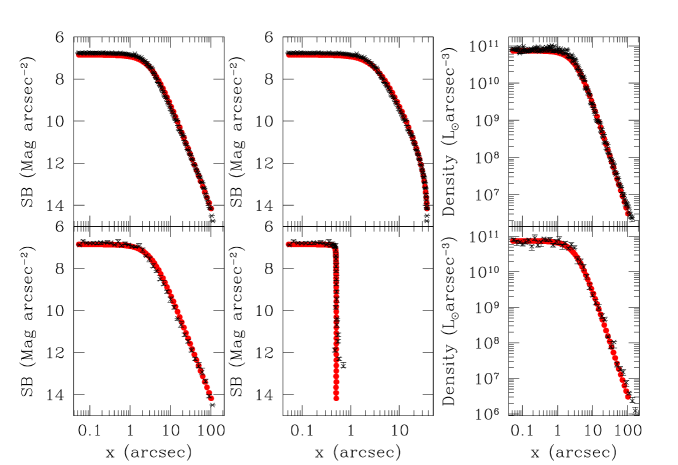
Figure 3: Figure to display the performance of DOPING in the simulated test cases Test I (a disk galaxy with a round ellipsoidal centre that extends to only about 0.^′′5) in the lower panels and Test II (an elliptical galaxy with varying eccentricity) in the upper panels. The chosen analytical density distributions is shown in red open circles, as a function of the major axis coordinate, in the right panels. This known density, along with the eccentricity profile shown in Figure 2, implies the surface brightness distributions which are shown in red along different azimuths $\phi$, (major axis, minor axis), in red filled circles, in the left and middle panels. The recovered density distributions along the major axis are over-plotted on the known density profiles, in black, in the right panels. Projections of these recovered density distributions are shown in black, as functions of $x$ along two different azimuths ($\phi=0$, i.e. major axis and $\phi=90^{\circ}$, i.e. minor axis), superimposed on the brightness data along these respective azimuths. The sharp rise of the eccentricity profiles in the two test cases (over length scales that are a factor of 80 apart) is indicated by the much sharper decline of the density along the minor axis, compared to the major. Higher regularisation is implemented in the recovery of the density distribution in the Test II case than in the case of Test I. In this figure, as well as in all subsequent figures, we assume that the surface brightness is measured in the SDSS $z$-band for a galaxy at a distance of 17Mpc. This is true unless otherwise stated.

The robustness of the comparison between the test 2-D brightness distribution of the test galaxies and the projections of the recovered density distributions is brought out in Figure 4 and Figure 5.

Figure 4: Left: the 2-D surface brightness (in mag/arcsec²) distribution of our flat test galaxy Test I, as a contour plot on the plane of the sky ($x-y$ plane). The contours in broken lines pertain to the toy brightness data that was fed into DOPING while the solid lines represent the projection of the 3-D luminosity density that DOPING recovers. The gap around $y$=0 occurs in the distribution of the projected density since the smallest (logarithmic) spatial bin is about 1pixel, i.e. 0${}^{{}^{\prime\prime}}$.05. Right: same as for the left panel, except that in this case, the central rounder part of the test galaxy has been focused upon.

Figure 5: 2-D surface brightness (in mag/arcsec²) distribution of the elliptical test galaxy Test II, compared to the plane of the sky projection of the luminosity distribution recovered by DOPING for this system.

The recovered density profile as well as its projection appear to tally very favourably with the known distributions.

3.2 Changing Inclinations

In this section, we investigate the extent to which the recovered luminosity density is rendered uncertain by our ignorance of the inclination angle $i$, under a given assumption about the geometry of the system and for a given set of observables.

In order to track this uncertainty, we use the test surface brightness data given in Equation 11, and constrain the projected eccentricity to be radially invariant: $e_{p}=e_{p0}$. Working with a constant $e_{p}$ is preferred to a radially dependent projected eccentricity, on grounds of ease of interpretation of the results. The deprojection of the test galaxy is performed under the assumption that the galaxy is oblate in shape. For such a geometry, the inclination cannot be less than $\sin^{-1}e_{p0}$.

We perform a suite of deprojections of the test surface brightness data with $i$ set to $i_{1},i_{2},i_{3},\cdots,90$^∘, where $i_{1}$ is the minimum inclination consistent with the observed projected eccentricity of $e_{p0}$, i.e. $i_{1}=\sin^{-1}e_{p0}$. Here $e_{p0}$ is chosen to be one of the following 4 values: $e_{p0}=0,0.71,0.87,0.95$. These values of $e_{p0}$ were chosen to span the range that early type galaxies are typically observed to bear. Deprojections were performed for each $e_{p0}$, at each of the 4 selected $i$. Thus, our experiments can track 4 test galaxies which are distinct in their flattening, each assumed oblate and viewed at a suite of different inclinations, the smallest of which is set by the projected eccentricity.

Figure 6 shows the density profiles recovered by DOPING by deprojecting the test surface brightness (Equation 11), for the choice of $e_{p0}$=0.71. This corresponds to $i_{1}\approx 45$^∘. For this configuration, deprojection is performed at four distinct values of the viewing angle, in the range of [45^∘, 90^∘], at $i\approx 46\hbox{${}^{\circ}$},\leavevmode\nobreak\ 48\hbox{${}^{\circ}$},\leavevmode\nobreak\ 55\hbox{${}^{\circ}$},\leavevmode\nobreak\ 90\hbox{${}^{\circ}$}$. It is possible to obtain the given surface brightness map that manifests a given projected flatness ($e_{p0}$=0.71) at these 4 different inclinations, only by projecting the luminosity densities of 4 distinct oblate galaxies with intrinsic eccentricities of 0.99, 0.95, 0.87, 0.71.

Thus, deprojection of the observed brightness map, carried out at varying inclinations, is characterised by variation in amplitudes as well as shapes. However, it is only along the major axes (the semi-axis along $\hat{x}$) that the deprojected profiles will appear similar in shape but different in amplitude. This owes to our definition of the toy surface brightness distribution (Equation 11). Along all other directions, the recovered density distributions will manifest differences in shape as well. It is for this reason that in Figure 6 we present the recovered density profiles along the galaxy minor axes. The variation in shape across the set of deprojected density profiles is clear from this figure.

It is to be noted that the projections of the recovered density profiles coincide with the input surface brightness data in each case. However, once $i\leq 58$^∘  (for projected eccentricity =0.71), the 3-D density profiles become a sensitive function of $i$. As expected, the recovered density is maximum (at every radius) when the intrinsic eccentricity is highest (i.e., the inclination angle is lowest). When the galaxy is assigned an even higher projected eccentricity, the uncertainty in the obtained density shows up at even lower $i$, i.e at inclinations closer to the face-on configuration.

Figure 7 presents the value of the recovered luminosity density at the innermost radial bin (about 0.^′′05), plotted as a function of the assumed inclination, for varying values of the intrinsic eccentricity, under the assumption of oblateness. As expected, the central density values concur (within the error bars), for the edge-on configuration, while density is highest at the centre at $i=0$^∘ , for the intrinsically most eccentric system.

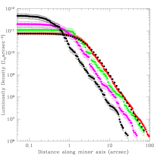
Figure 6: Figure showing luminosity density distributions recovered by deprojecting the surface brightness profile given by Equation 11, under the assumption of oblateness, given a projected eccentricity of 0.71, viewed at inclinations of about 46^∘ (in black), 48^∘ (in magenta), 55^∘ (in green) and 90^∘ (in red). The recovered density distributions are plotted along the minor axes. The true luminosity density of the test galaxy is shown in filled black circles. The profiles above were recovered from runs performed with various bin widths ad smoothing parameter values. The estimation of the error bars on the recovered density profiles is discussed in Appendix D.1.

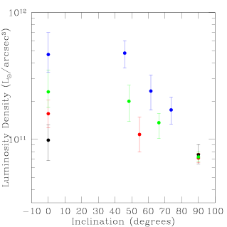
Figure 7: Central luminosity density, plotted as a function of inclination for four different values of the intrinsic eccentricity. When the intrinsic eccentricity is 0.71, the obtained central density points are shown in black. The colour coding for the other values of $e$ is as follows: $e$=0.87, 0.95 and 0.99 correspond to red, green and blue, respectively. The case of inclination=0 obviously indicates the situation when the observed isophotes are circular, i.e. the observed projected eccentricity is zero.

3.3 Changing Geometry

In the last section we explored how our unfamiliarity with the inclination of a galaxy can lead to a non-zero range of possible density profiles that a single observed brightness profile can correspond to. This range had been investigated under an assumption for the geometry of the galaxy, namely oblateness. In this section, we attempt to gauge the effects of treating an intrinsically oblate system, (our test system of Equation 10, conferred a constant $e_{p}$ of 0.99) as triaxial (with the photometric major axis along ${\bf{\hat{x}}}$ and LOS extent set to half the photometric major axis ), prolate and spherical, viewed at $i$=90^∘ (see Figure 8).

Assuming this rather flat test system to be oblate implies that $q_{1}$ is a constant, =1 and $q_{p}=1/\sqrt{1-e_{p}^{2}}\approx 7.1$ (where we have used our definition of $q_{1}$ and $q_{p}$, as given in Appendix C). Then from Equation 4 we get that for $i$=90^∘, $q_{2}\approx 7.1$. Similarly, when the system is assumed prolate, $q_{1}$=1, $q_{p}=\sqrt{1-e_{p}^{2}}\approx 0.14$ and $q_{2}\approx 0.14$. When we assume the system to be triaxial as above, then for $i$=90^∘, $q_{LOS}$=0.5 and $q_{p}\approx$7.1, $q_{2}\approx$7.1 and $q_{1}$=2.

When we input these different values of $q_{2}$ in Equation 5, we get values of $z_{max}^{jk}$ from the oblate case that are different from what we get for the prolate case. In fact, for edge-on viewing, as in here, for a given $k$, the maximum $z$-height attained by any point in the $k^{th}$ isophotal annulus is higher for the oblate case than the prolate case. As a result, the density distribution that is recovered from the oblate case is lower in amplitude than that from the prolate case. The triaxial case result falls in between that from the oblate and prolate cases.

In the case of galaxy clusters, when $q_{LOS}$ information is available, DOPING can be called in to perform deprojection in the fully triaxial geometry without requiring to make any assumption about one of the intrinsic axial ratios (Chakrabarty, de Filippis and Russell, 2008).

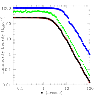
Figure 8: Luminosity density of our oblate test galaxy of projected eccentricity 0.99 (shown in red), recovered by DOPING, under the assumptions of prolateness (in blue), oblateness (in black) and triaxiality with ratio between LOS extent and photometric major axis = 0.5 (in green). All the deprojections were carried out for an edge-on viewing.

3.4 Effect of PSF

We hope to use DOPING to extract luminosity profiles of real galaxies, in particular, the ACS VCS galaxies. It therefore becomes important to gauge the effect of the ACS PSF on the recovered density. This is done by convolving the projection of the density in any iterative step with the ACS PSF and comparing this convolved profile to the observed surface brightness. The result is shown in Figure 9. As indicated in the figure, the effect of the ACS PSF does not extend beyond the central few arcseconds (in fact, 10${}^{{}^{\prime\prime}}$).

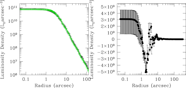
Figure 9: Left: luminosity density of an oblate test galaxy with uniform eccentricity of 0.99, recovered by comparing the input brightness profile with the PSF convolved projection of the density in any iterative step. The PSF in question is the ACS PSF in the F850W filter. When the convolution with the PSF is ignored, the recovered density is shown in green. Right: difference between the density profiles obtained with and without convolving with the PSF. It is noted that inside the central 10${}^{{}^{\prime\prime}}$, this difference is 2 orders of magnitude less than density while outside 10${}^{{}^{\prime\prime}}$, the difference tends to zero.

4 Applications to real systems

In this section, we demonstrate the application of DOPING to real galaxies. The efficacy of DOPING in dealing with galactic systems that vary over wide ranges of magnitudes and morphology - including a nucleated disky galaxy - is advanced with applications made to the observed galaxies Ic 3019 and Ic 3881. In addition, the recovery of the density for the cluster A1413, without resorting to assumptions about geometry and inclination, is also included.

4.1 Ic 3019 - effect of smoothing

Here we apply DOPING to deproject the measured surface brightness map of the galaxy Ic 3019 (vcc9) which is observed within the ACS VCS (Ferrarese et al. 2006). In particular, the effect of the smoothing parameter $\alpha$ is demonstrated in the context of this example galaxy. Thus, this section also brings out an application of DOPING to the analysis of real data. This galaxy is low on brightness and the reason for choosing it is to adduce evidence for the wide range of systems that DOPING can tackle.

The eccentricity of this galaxy has been measured to vary with radius, though not radically, under the ACSVCS observational program. In fact, eccentricity has been reported to be uniform at about 0.85 till about 2.5^′′, from which it drops abruptly to about 0.3 at about 6^′′, to undulate its way up to about 0.7 at about 200^′′.

The density distribution recovered for Ic 3019 is projected along the LOS and is plotted as a function of $x$ in Figure 10 in black, on top of the observed brightness data for vcc9. The three panels correspond to runs performed with three increasing values of the regularisation parameter $\alpha$, namely $\alpha$=0 (i.e. no smoothing), $\alpha$=0.1 and $\alpha$=1. Increasing $\alpha$ beyond this value did not make a significant change in the estimated density. The procedure to choose $\alpha$ is discussed in Appendix E.

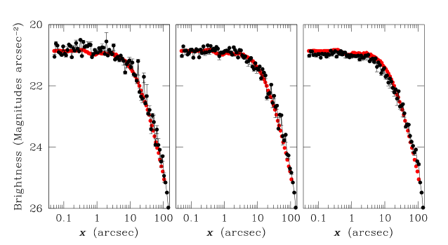
Figure 10: Figure to exhibit the effect of increasing the smoothing parameter $\alpha$, on the recovered density and hence its projection, which is plotted here in black, as a function of the major axis coordinate, over the brightness data for I3019 (vcc9), as was observed within the ACS VCS program (in red). As we proceed from left to right, $\alpha$ goes as 0, 0.1 and 1.

The projection of the recovered density distribution on the plane of the sky, is compared to the surface brightness map of IC 3019 in Figure 11.

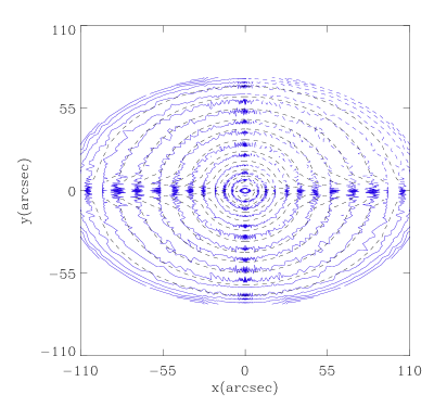
Figure 11: As in Figure 5, except that in this case, the plane of the sky brightness distribution of the galaxy IC 3019 is shown.

4.2 Galaxy cluster

In this section we discuss the results of applying DOPING to extract the X-ray luminosity density of the cluster A1413. The important feature about recovering the 3-D density of clusters with DOPING is that the true axial ratios and inclination can be constrained along the lines advanced by Chakrabarty, de Filippis $\&$ Russell (2008), as long as $q_{LOS}$ of the system can be estimated from the available SZe measurements. The cluster A1413 was reported in Chakrabarty, de Filippis $\&$ Russell (2008) to be a triaxial system with the intrinsic axial ratios of 0.96 and 1.64 and inclination lying between 66^∘ and 71^∘.

This configuration was identified upon deprojecting the X-ray surface brightness at four benchmark deprojection scenarios, namely oblateness and $i=i_{min}$, oblateness and $i=90^{\circ}$, prolateness and $i=i_{min}$, prolateness and $i=90^{\circ}$. Here $i_{min}\approx 47^{\circ}$ is the minimum inclination possible under the assumption of oblateness, given a projected axial ratio (= 1.473 for A1413). Inter-comparison of the 3-D density profiles recovered under these four scenarios leads us to the aforementioned prediction. Since the relative extent along three mutually orthogonal axes are known in this case, 3-D modelling is possible, i.e. the true geometry of the system can be estimated. Thus, we do not need to assume any axial ratio or inclination value. The density profile recovered under deprojection in the identified system geometry is presented in Figure 12.

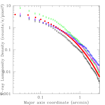
Figure 12: X-ray luminosity density profile of cluster A1413, recovered under the true system geometry ($q_{1}$=0.96, $q_{2}$=1.64) and inclination = 68.5^∘, i.e. the medial value of the identified range (as found by Chakrabarty, de Filippis $\&$ Russell, 2008), is plotted in red. The other profiles mark the densities recovered under four distinct assumptions about the system geometry and incinations - the four benchmark deprojection scenarios (see text in § refsec:A1413) used in Chakrabarty, de Filippis $\&$ Russell (2008).

4.3 2-component Galaxies

It is possible for DOPING to perform the deprojection of a bulge+disk galactic system in an integrated, single step fashion. This is made possible by ascribing two distinct seeds to the two components, namely the central bulge/nucleus and the more extended outer component upon which the central component is superimposed. The deprojection of the nucleated galaxies in the ACS VCS sample has been undertaken in Chakrabarty $\&$ McCall (2009, under preparation). An example of the deprojection of the surface brightness profile of such a 2-component, nucleated galaxy is shown in Figure 13.

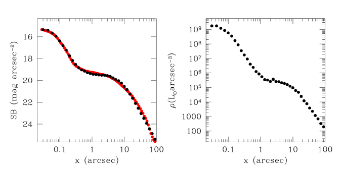
Figure 13: Luminosity density of the two-component galaxy Ic 3881 along the ${\bf{\hat{x}}}$-axis (right) and its projection (left) in black with the observed surface brightness data superimposed in red.

5 Discussions $\&$ Summary

In this paper, we have presented a fast (a typical run takes about two minutes on an Intel Xenon 3.2GHz CPU processor) new non-parametric algorithm, DOPING, that works via a penalised likelihood approach. It attempts to deproject the observed surface brightness profiles of galaxies, in general triaxial geometries, while taking into account intrinsic variation in shape.

The algorithm was successfully tested on toy galactic systems of varying morphologies, including an extreme system that was ascribed a small ellipsoidal bulge-like inner component that lay embedded in a highly flattened outer disk. Other experiments were best served by simulated galaxies with constant ellipticities. The code was also applied to a dwarf elliptical galaxy Ic 3019 (vcc9) and another dE, nucleated galaxy Ic 3381 (vcc1087) from the ACS Virgo Cluster Survey (Côté et al. 2004). An application to a real galaxy cluster, A1413, is also included.

5.1 Superior Design

The well-defined, inherent convergence criterion of DOPING, buffeted by the sophisticated MCMC optimiser renders it superior to other well used inverse deprojection scheme, namely the Richardson-Lucy algorithm. Besides, the nonparametric inverse design of DOPING helps it avoid risky practises such as parametric fitting, interpolation, etc. Finally, none of these methods can perform deprojection under generalised triaxial geometries, like DOPING can.

Choosing the LOS coordinate or $z$ as the basis for the density helps to keep the code modular. As a result, DOPING can handle deprojections in general geometries. The current version of DOPING relies on the determination of the intrinsic shape parameters (axial ratios) from measurements only of projected shape parameters. Such a relation is possible for unknown inclinations, only if the object shape bears a certain regularity. It is this that causes 3-D modelling with DOPING to be restricted to only objects with $m$-fold symmetries.

Thus, when the inclination is unknown but the relative extent along three mutually orthogonal axes are known, DOPING can handle an assortment of 3-D shapes that resemble $m$-winged star-fruit-like shapes, the 2-D projections of which are $m$-pronged star-fish-like 2-D shapes. Such generalised geometries can be described by the 3-D extension of Gielis’s “superformula” (Gielis 2003). The superformula is a 6-parameter generalisation of the superellipse (which are the Lame’ curves with unequal semi-axes). In fact, the product of two superformulae - one corresponding to a generalised superellipse in the $Z$=0 plane and another in the $Y$=0 plane - can give rise to the $m$-winged star-fruit-like 3-D shapes.

However, a more generalised version of DOPING that allows fast and robust three dimensional modelling in unrestricted geometries is also possible - only in situations in which the system can be viewed at multiple inclinations. Such configurations are not of astronomical context but bear strong application potential; this will be reported in a future contribution.

5.2 DOPING Deals with Substructure

Continuing on the issue of code generality, we recall that in §4.2 it was shown that DOPING can deal with galaxies, the light distribution of which betray a bulge+disk structure. In fact, DOPING is capable of deprojecting systems marked with multiple structures that may not necessarily be concentric. As long as the centres of each component are known, the algorithm can be employed for deprojection.

5.3 Why Choose ${\hat{\bf X}}$=${\hat{\bf x}}$

In general, there will be two angles involved in the rotation matrix that connect the the two Cartesian coordinate frames. However, when we speak about inclinations of observed astronomical systems, we typically specify one angle of inclination for a given system. In other words, it is modelled that one of the two angles of inclinations is set to zero, while the angle between a principle axis of the system and the LOS is advanced as the inclination $i$. Given that the image plane is what is fixed by observations - and therefore the LOS - one of the system principle axes (one that we refer to as the $Z$-axis, say) can be at angle $i$ with the LOS, i.e. ${\hat{\bf Z}}$ can lie anywhere on the surface of a cone that has an axis along the LOS and a semi-angle $i$. There is no observational constraint that can restrict our choice of the location of ${\hat{\bf Z}}$ on the surface of this cone. For a given choice of this location, the $X-Y$ plane is fixed accordingly. The choice that we make in this work, corresponds to ${\hat{\bf X}}$=${\hat{\bf x}}$.

It is true that the recovery of the 3-D density distribution could be affected by a different choice for the location of ${\hat{\bf Z}}$ on the surface of the cone. This is so because the system at hand is triaxial in general, rather than axisymmetric. At the same time, we need to appreciate that there is no observational information that would inspire a particular choice. Hence we adopt the choice that eases calculations, keeping in mind the fact that as a consequence of this, the recovered 3-D density structure is one possible answer for a given surface brightness data. Of course, we could undertake deprojection for other non-zero values of $\cos^{-1}{\hat{\bf X}}\cdot{\hat{\bf x}}$. In fact, a band of uncertainties on the recovered 3-D density can be derived, corresponding to varying choices of this angle, though no “most-likely” region for the density can be identified within this band. However, given the state of equally poor constraint on the density, the solution corresponding to one given value of the azimuthal inclination is advanced here.

The other assumptions that we make about geometry and inclination - provided by the user as inputs into the code - can be varied and the corresponding range of recovered 3-D density distributions can be recorded, with ${\hat{\bf X}}$ always assumed equal to ${\hat{\bf x}}$. This is particularly easy, given the short run-times of a typical run of DOPING. It is important to stress here that our assumptions are not invoked to cover for flaws in algorithm design but are essential in order to render the deprojection scenario unique, i.e. to ascertain the deprojection geometry and inclination. Our assumptions merely compensate for the lack of (observational) information about such deprojection scenarios.

Given the assumptions that we need to make, the question that may be asked is if the proposed ambition of DOPING to deproject in triaxial geometries is inane, in that it is driven by unconstrained assumptions. Such a worry has been addressed in the beginning of §2 and discussed later in § 5.5. In the following section, we elucidate the follies of assuming axisymmetry, given observations on galactic systems, thus, reinforcing the need for invoking triaxiality.

5.4 The Folly of Axisymmetry

A general non-irregular galaxy, whether elliptical or axisymmetric, can be approximated as a triaxial ellipsoid (the third axis is tiny in a disk system, compared to the other two intrinsic axis lengths). The modular structure of DOPING allows for deprojection of galaxies of both elliptical and disky morphologies. As discussed above, other deprojection methods can at most imply axisymmetry.

However, often, the assumption of axisymmetry (Magorrian 1999, RK) is not just a mild deviation from the truth but is plain wrong - this is clear in the cases of inclined, disk-like systems. In these systems, while the extent along the perpendicular to the disk is much smaller than that along the other two axes in the disk, a non-zero projected ellipticity ($\epsilon$), measured on the plane of projection implies that in general, both intrinsic axial ratios - and particularly the ratio of the principal axes in the disk - deviate from unity. A few examples of such systems from the ACS Virgo Cluster Survey (Ferrareseet al. 2006, web site of ACS Virgo Cluster Survey Databases) include:

• NGC 4382 (or vcc 798, SA galaxy) in which $\epsilon$ ranges from 0.6 at the centre to 0.2 outside,

• NGC 4762 (or vcc 2095, SB) in which $\epsilon$ approximately increases to 0.4, starting from about 0,

• NGC 4442 (or vcc 1062, SB) in which $\epsilon$ increases outward to 0.6 from about 0,

These examples bring out the fact that axisymmetry is not an acceptable approximation but an excuse for a scheme that fails to incorporate an improved alternative. Of course, in lieu of information along the LOS, even under the assumption of axisymmetry, some assumption has to be made about the intrinsic axial ratio. If the inclination permits a good estimate of the same, then no such assumption needs to be resorted to, whether with assumed axisymmetry or with DOPING.

5.5 Justification of Assumptions

The solution that we will achieve for the most likely 3-D density, given the surface brightness data, will depend on the assumptions that we use for the unconstrained inclination and the axial ratio. Of course, such assumptions will call for physical justification - however, the fundamental issue here is that for galaxies, there is no observational evidence that will constrain such assumptions. For galaxy clusters, the availability of the maximum extent along the LOS, (from SZe measurements), definitely helps to constrict the number of assumptions that we then need to make (see Appendix B). Similarly, for systems which can be viewed at selected inclinations, 3-D modelling is rendered robust and fast. Again, for flattened systems, we can estimate one of the inclinations and therefore deprojection then entails one less assumption. However, the lack of sufficient physically relevant measurements means that assumptions invoked to characterise a general triaxial system cannot be justified to satisfaction. In lieu of this, all that DOPING can offer is a fast estimate of the range of density distributions obtained over the considered range of axial ratios and inclinations. Turning this argument around, we realise that the range of 3-D density distributions that are recovered in §3.2 and 3.3, for distinct geometry+inclination inputs (assumptions) cannot be narrowed down for general triaxial galactic systems.

The question that then begs addressing is if deprojection in triaxial geometries is any improvement upon the existing deprojection routes that are currently in vogue. That the need for triaxiality over axisymmetry, is physically justified, was delineated in the last sub-section. However, given the dearth of observational information - particularly for galaxies rather than galaxy clusters, as discussed in § 2 and above - assumptions need to be invoked. The superiority of DOPING lies in the fact that when information about intrinsic morphology and inclination are less sparse than for galaxies (as for clusters or deposited nano-particles), identification of the true triaxial geometry is possible (Chakrabarty, de Filippis $\&$ Russell 2008) and deprojection can then be performed in this geometry, without invoking assumptions about $i$ and $q_{1}$ (as demonstrated for the Abell cluster A1413 in § 4.2).

5.6 Position Angle

Had the two angles of inclination been known to us, we would be in a position to predict the observed projected position angle as a function of these inclinations. However, given the projected position angle, constraining the inclinations requires an inverse approach, which is possible within DOPING in the triaxial geometry. We could then relax the assumption of ${\hat{\bf X}}$=${\hat{\bf x}}$ while continuing to assume the polar inclination angle. In fact, the coordinate system (and the ensuing equations) used here is a limiting case of the assumption of a non-zero, radially varying position angle. In this more generalised version of DOPING, the angles between $\hat{\bf x}$ and the line of nodes will be non-zero and varying with radius (Simonneau, Varela $\&$ Munoz-Tunon 1998). This will be dealt with in a future contribution.

When the position angle is included in the calculations the data table is enhanced by another column yet - $\phi_{0k}$, where $\phi_{0k}$ is the position angle of points in the $k^{th}$ isophotal annulus. Then, the body coordinate system corresponding to the $k^{th}$ isophotal annulus is rotated by $\phi_{k0}$ with respect to the $\phi$=0 line, i.e. the $x$-axis (by definition), so that the new body coordinate system governing the triaxial shell - the largest projection (of the same thickness as itself) of which is the $k^{th}$ isophotal annulus - is given by $X^{\prime}-Y^{\prime}-Z^{\prime}$, where:

$$X^{\prime} = X\cos\phi_{0k}+Y\sin\phi_{0k}$$ (12)

$$Y^{\prime} = X\sin\phi_{0k}-Y\cos\phi_{0k}$$ (13)

$$Z^{\prime} = Z$$ (14)

Having established this, the equivalent of Equation 5 can be written down. The reformed equation is still a quadratic and is solved for the two solutions of $z$ as before. In the present calculations, we avoided this extra complication in light of the small isophotal twist observed with the ACS VCS galaxies, which are the prime targets of the discussed code.

5.7 Effect of Seed Selection

Our starting luminosity density is motivated by crude estimates of the sought function (Gelman et. al 1995); we are guided by the requirement that the projection of the seed density be close to the given surface brightness data. The algorithm will indeed fail to converge for completely irrational choices of the initial parameters (steepness parameter $\gg 1$, scale length different from the correct choice by more than 4 orders of magnitude). Importantly, under such circumstances, the projection of the recovered density will be found to deviate from the brightness data. Additionally, it may be remarked that it is reasonable to start with a steepness parameter that is close to unity and a scale length that is of the order of the core radius that characterises the surface brightness profile of the system. Given that a typical run takes less than 2 minutes on an Intel Xenon 3.2GHz processor, it is feasible to restart the algorithm for a different choice of the initial guess, until convergence is reached.

5.8 Effect of Data sampling

We also note that the spatial sampling of the data can have some effect on the density distribution recovered by DOPING. For instance, in Figure 14, the density profile best reproduces the data at small, rather than large radii. This is a consequence of the fact that, by construction, our simulated data set happens to have substantially more data points in the inner regions of the galaxy than on the outside, with the consequence that the innermost region has larger weight in driving convergence.

6 Conclusion

Thus, DOPING is advanced as a simple but powerful deprojection algorithm, that can be treated as a black-box by the user, is fast and offers 3-D density distributions in general geometries, without resorting to making unconstrained approximations to the form of the density or blindly accepting validity of commonly used goodness of fit measures in light of the inhomogeneous errors of measurement (Bissantz & Munk 2001).

The greatest novelty borne by DOPING is its applicability to general systems. Even though in the above examples, triaxial systems were investigated - ranging from razor thin discs to 2-component or bulge+disk galaxies - even when inclination is unknown DOPING can deal with all systems that offer an analytical relation between the intrinsic and measured projected shape parameters. The class of geometries that bear an $m$-fold symmetry allows for this. 3-D modelling of images of systems with even more general geometries can also be performed with DOPING, as long as the system can be imaged at various known inclinations. That deprojection into the third dimension is possible in such general geometries, in a non-parametric way, is due to the fact that the representation of the sought density is modular, i.e. not dependent on a characteristic of the system geometry.

The recovery of the 3-D density is performed iteratively, by searching for the most likely 3-D density structure that projects to the observed 2-D image. This search is robustly undertaken by an MCMC optimiser. Since the choice of the 3-D density is constrained via its projection, distinct 3-D density distributions will project to the same 2-D image. To lift this degeneracy, in DOPING, the system geometry and orientation are specified completely. That axisymmetry is an invalid assumption - at least in real disc-like galaxies - was shown above. Consequently, the description of galaxy geometry as triaxial is a suitable alternative. However, triaxiality entails two axial ratios and inclinations, not all of which can be specified, given the constricted level of achievable observed information. When observed information is available, DOPING can perform deprojection under triaxiality without invoking assumptions, while in lieu of the same, assumptions are invoked. The former case is demonstrated above via the example of deprojection of a galaxy cluster. A benefit of the speed of the algorithm is that a suite of 3-D density models, corresponding to a range of assumed values, is achieved quickly.

Thus, the strengths of DOPING include generalised applicability, ability to incorporate substructure and non-parametric density recovery, along with logistical advantages such as high speed of runs and user-friendliness. Such characteristics render DOPING a very useful tool in three dimensional modelling. In particular, the all important estimation of galactic masses will be aided by a tool such as DOPING.

Appendix A Representing isophotes

The shape parameters of the isophotes form the input information, so we can formulate smooth analytical approximations to the isophotes. Of course, it is the fitting of such smooth approximations to the surface brightness data that provides estimates of the isophotal parameters; in other words such approximations are readily available. It is to sort grid points on the image plane, into respective isophotal annuli, that we invoke these approximations. However, real isophotes can be irregular and not altogether smooth. To take this into account, we examine the isophotes first and estimate the typical length scale over which the irregularity in the isophotes occurs. Thus, for example, the isophotal contours of a distant galaxy could be imaged by a given instrument as more jagged than those of a nearby system. We discard grid points on the image plane that lie within this estimated spatial range corresponding to deviations from smoothness.

Appendix B Specifying the system geometry for triaxial galaxies

The specification of triaxiality of an example galaxy entails knowledge of:

• 2 constant intrinsic axial ratios $q_{1}$ and $q_{2}$ for systems with radially independent shape. Alternatively, for systems with radially varying intrinsic eccentricities - 2 intrinsic axial ratios that vary as known functions of distance away from centre of system.

• 2 position angles or inclinations.

Of these, we

• set one inclination angle to 0 by setting one photometric axis (along the ${\hat{\bf x}}$-axis) to be coincident with an intrinsic principal axis (see § 2.1).

• assume a value for the other inclination $i$.

• derive the two intrinsic axial ratios from the two projected axial ratios:

  1. ratio of the photometric semi-axes ($q_{p}$).

  2. ratio of the semi-axes along the LOS to that along the photometric major axis ($q_{LOS}$).

However, generally we cannot measure the extent of a galaxy along the LOS. This is not so for other systems though, eg. galaxy clusters, the LOS extent of which is constrained by SZe measurements; for such systems, we can solve for $q_{1}$ and $q_{2}$ from:

• $q_{p}=f_{1}(q_{1},q_{2},i)$ and

• $q_{LOS}=f_{2}(q_{1},q_{2},i)$,

where $f_{1},f_{2}$ are analytical functions whose forms can be derived from geometrical considerations. In lieu of the measure of the system along the LOS, we compensate for our ignorance of $q_{LOS}$ by assuming one of the intrinsic axial ratios ($q_{1}$). Then using this assumed $q_{1}$, we can obtain $q_{2}$. With $q_{LOS}$ available, deprojections of X-ray brightness data of clusters have been performed by DOPING in triaxial geometries, without requiring any assumption for $q_{1}$ (Chakrabarty $\&$ de Filippis, under preparation).

Appendix C Axial ratios

We clarify that the axial ratios $q_{2k},q_{1k},q_{pk}$ are defined such that the extent along $\hat{\bf x}$ is in the numerator. Thus,

• $q_{pk}$ is the ratio of the semi-axis along $\hat{\bf x}$ of the $k^{th}$ isophotal annulus, to that along $\hat{\bf y}$, on the image plane.

• $q_{2k}$ is ratio of the semi-axis along $\hat{\bf x}$ to that along the $\hat{\bf Y}$.

• $q_{1k}$ is ratio of the semi-axis along $\hat{\bf x}$, to that along the $\hat{\bf Z}$.

where $\hat{\bf x}=\hat{\bf X}$ (see § 2.2).

In the examples shown later in the paper, we assume the system to be oblate, unless otherwise stated, i.e. then $q_{1k}$ is a constant, (=1) and $q_{2k}>$ 1. If we are considering a prolate system, then $q_{1k}$ is again a constant, (=1) but then $q_{2k}<$ 1.

Appendix D Optimisation

We seek solutions for $\rho$ that correspond to the $\pm$1-$\sigma$ neighbourhood of the global maxima of ${\cal{L}}$ and employ an MCMC optimiser for this. The particular implementation of this in our work is the Metropolis Hastings algorithm. Once Metropolis-Hastings attains the equilibrium stage, it moves around in the maximal region of ${\cal{L}}$. During this stage the average of an ensemble of models should represent the distribution that is to be sampled; this is reflected in stationarity in the trace of the likelihood. Before recording the solutions, we typically allow for 5 times the period of burn-in to lapse, mindful of the fact that burn-in can continue much longer than suggested by the trace. Details of the optimisation are presented in Gelman, Roberts $\&$ Gilks (1996); Roberts, Gelman & Gilks (1997); Roberts and Sahu (1997); Roberts & Rosenthal (2001).

We use circular iterations, with the 1^st to the $N_{iter}^{th}$ iterative step repeating in cycles. We define convergence as when inside the equilibrium stage, the likelihood attained in the $i^{th}$ step during the $M^{th}$ cycle, falls below the likelihood attained in the $i+1^{th}$ step during the $M-1^{th}$ cycle. It is expected that then the algorithm has indeed passed through the global maxima in the likelihood. The extent of wandering of Metropolis in this maximal region is a direct measure of the errors of the analysis.

D.1 Uncertainties

In fact, when we say that the errors of our analysis are quantified by the $\pm$1-$\sigma$ spread across the ensemble of identified density values, we actually imply a as 68$\%$ interval. To expound on the procedure of quantifying the errors: at a point $(x,y,z)$, the values of the luminosity density corresponding to the maximal region of the likelihood function are recorded. This vector of density values is sorted and values at the 16^th, 50^th and 84^th centiles are noted. The interval estimate of the luminosity density at this given point $(x,y,z)$ is then represented by the error band bound by values corresponding to the 16^th and 84^th centiles; the density value at the medial position within this interval is also shown within this error band.

D.2 Updating Density

At the beginning of every step, each $\bf{z-histogram}$ is varied, independently of each other, while maintaining the realistic conditions of positivity. In general, the old value of the relevant variable ($X$) in step $i$ is related to a new value $Y$ in the next step: $Y=X+Z$, where $Z$ is a random variable. A variety of proposals to move from $X$ to $Y$ are described in the literature (Mengersen & Tweedie 1996; Gelman, Roberts $\&$ Gilks 1996). Of these, we choose that the algorithm proposes to move from $X$ to $Y$ using the random walk jumping distribution, i.e. $Y=X+sU$, where $U$ is a Gaussian random deviate and $s$ is the scale parameter that determines the size of the jump. If the amount of change is very small, the chain will require a very large number of steps to become well-mixed and hence efficiency will be compromised. If the step-size is too large, the worry is that the resulting configuration will miss the global maximum and fall into regions of very low likelihoods, wasting a number of steps in the process (Draper 2000). Our chosen jump proposal is adaptive in nature since the updating of $\rho(\cdot)$ at a given $z$, depends on the density at that $z$. The details of the density updating is as follows:

$$\rho_{n+1}(x_{k}^{j},y_{k}^{j},z_{l}) = \rho_{n}(x_{k}^{j},y_{k}^{j},z_{l}+\delta{z})+\Delta_{l}R\quad{\textrm{where}}$$

$$\Delta_{l} = \rho_{n}(x_{k}^{j},y_{k}^{j},z_{l})-\rho_{n}(x_{k}^{j},y_{k}^{j},z_{l}+\delta{z})$$ (15)

$(x_{k}^{j},y_{k}^{j},z_{l})$ in step $n$. Also, $R\sim N(0,scl_{1}^{2})$ and $scl_{1}$ is a scale that determines the extent of the jump in the shape of a ${\bf z-histogram}$ between two consecutive steps. Also, for this $k,j$, $z_{l}$ is the $l^{th}$ $z$-bin and $z_{l+1}=z_{l}+\delta{z}$. This updating is done $\forall\>l:z_{l}\in[0,z_{max}^{jk}]$, $\forall\>j,k$, to accomplish change of shape of the ${\bf{z-histogram}}$ corresponding to the $j,k$.

We still need to make a change to the overall amplitude of the new density distribution. This is done by scaling $\rho_{n+1}(x_{k}^{j},y_{k}^{j},z_{l})$ by another random deviate $\sim N(0,scl_{2}^{2})$, $\forall\>l$; here $scl_{2}$ is another scale that determines the amount of change of amplitude that is brought about in the density structure, for a given $j,k$.

The values of $scl_{1}$ and $scl_{2}$ are arrived at experimentally, keeping the effect of large and small scales in mind.

We choose to work with equal binning along all three coordinate axes; this binning is logarithmic in nature. A good choice for the smallest bin size is of the order of the spatial resolution of the data. A typical run takes about 2 minutes on an Intel Xenon 3.2GHz CPU processor.

D.3 Temperatures

The probability of accepting the proposed move from likelihood ${\cal{L}}(A)$ to ${\cal{L}}(A^{{}^{\prime}})$ is discussed here. Here $A$ generically represents the domain of the likelihood function which is the set of the ${\bf{z-histograms}}$ and $A^{{}^{\prime}}$ is the new set of ${\bf{z-histograms}}$ to which a move has been proposed.

Anxiety over multi-modality of the likelihood function has prompted us to work both with highly dispersed initial values (or seeds) to initiate multiple chains (Gelman $\&$ Rubin 1992) and also to use simulated annealing in a single chain. When the latter is implemented, the transmission probability is

$$P(A\rightarrow{A^{{}^{\prime}}})=min\displaystyle{\left[\exp{\frac{\Delta{\cal{L}}}{T}},1\right]},$$ (16)

where $\Delta{\cal{L}}=\ln{{\cal{L}}(A^{{}^{\prime}})}-\ln{{\cal{L}}(A)}$ and $T$ is the temperature parameter.

We have implemented both a uniform temperature profile, as well as played with a cooling schedule that starts with an initial temperature $T_{0}$ which is allowed to cool down to a final value of $T_{f}$, over a step number of $N_{cool}$. In practice, we choose $T_{f}/T_{0}$ to be 0.1 while $N_{cool}$ is typically set to double the number of steps that correspond to $burn-in$, as judged from traces of system characteristics, such as the value of the density that is recovered at a fiduciary location. We find that the answer depends only very weakly on the details of the cooling schedule.

Appendix E Choice of the Regularisation Parameter

Thomson et al. (1991) refer to the smoothing parameter as the compromise between “fidelity to the data and smoothness”. While different methods are suggested by Thomson et al. (1991) and Titterington (1988), to constrain the scalar $\alpha$, we choose to accept a value that is achieved via an empirical implementation of the minimisation of the total mean-squared error. We define the total mean-squared error (TMSE), for a given value of $\alpha$ as:

$$\delta_{\alpha}=\displaystyle{\frac{{\displaystyle\sum_{i=1}^{N}(\rho_{median}^{i}-\rho_{-1\sigma}^{i})^{2}}+{\displaystyle\sum_{i=1}^{N}(\rho_{median}^{i}-\rho_{+1\sigma}^{i})^{2}}}{2N}}$$ (17)

where there are $N$ grid points over which a density profile is recovered and $\rho_{median}^{i}$ is the density recovered at the medial level in the $i^{th}$ grid point, while $\rho_{-1\sigma}^{i}$ and $\rho_{+1\sigma}^{i}$ are the values recovered at the -1$\sigma$ and +1$\sigma$ error levels, respectively. We scan over a range of $\alpha$ values and stop increasing $\alpha$ when the smallest $\delta_{\alpha}$ is achieved. Typically, beyond a given value, increasing $\alpha$ maintains the corresponding value for TMSE. It is the smallest $\alpha$ at which this trend is noticed that is chosen as the $\alpha$ we use in the runs.

Appendix F Choice of Seed for Density

The robustness of a recursive formalism is reflected in the extent to which the initial guess for the solution is irrelevant to the final result. With this in mind, we undertook extensive experimentation with seed density distributions used by DOPING as starting guesses. For this investigation, we use the same simulated data set of an oblate galaxy, viewed edge-on, as described above: analytical density of Equations 10 and a constant eccentricity of 0.99.

Typically, we use a seed density $\rho_{seed}=\rho_{seed}(\xi)$, where $\xi$ denotes the ellipsoidal radius. In fact, we choose a seed density that has a form akin to the Lorentzian distribution:

$$\rho_{seed}(\xi)=\displaystyle{\frac{a}{1+\displaystyle{\left(\frac{\xi}{b}\right)^{2n}}}},$$ (18)

The three parameters in this distribution are

• the scale length $b$ which determines the width of the profile,

• the central density $a$ and

• an exponent $n$ that defines the steepness of the fall of the tail of the profile.

A reasonable starting value of $n$ is about 1. We find that of these three parameters the algorithm is least sensitive to the choice of the amplitude $a$. When the scale-length and the steepness parameter are widely varied, the algorithm also follows the input data, though it is more difficult for the code to do so for radical changes in shape than in amplitude. To test the robustness of DOPING to the initial guess, for each input parameter, we performed two runs with values chosen to be at opposite ends of the true value. The density profile that DOPING retrieves when $a$ is varied, is compared in Figure 14 to the known density distribution. The projections of the density profiles are also shown, superimposed on the brightness data that serves as the input to the code.

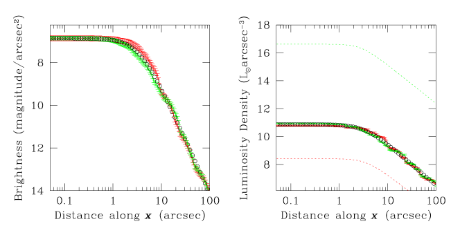
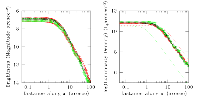
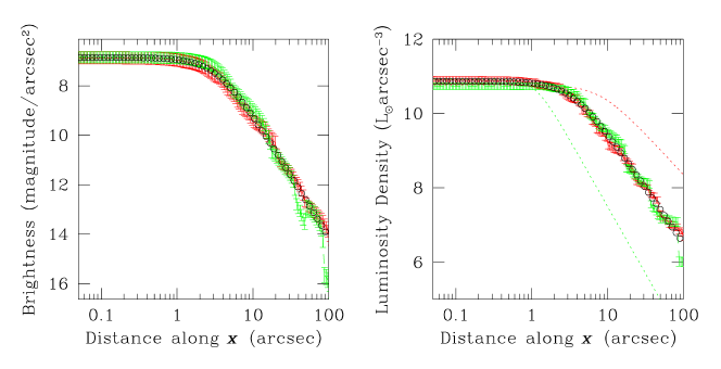
Figure 14: Top row: figure to verify the robustness of DOPING to changes in the central density of the initial guess for the density distribution. Density profiles from two runs (in red and green, superimposed with error-bars), performed with values of the central density parameter that are apart by eight orders of magnitude, are shown in the right panel. Superimposed on these is the true density of the system, shown in black open circles. The initial seeds for the density distributions in the two runs are shown in dotted lines, in the corresponding colours. The left panel shows projections of the recovered density profiles in corresponding colours, with the input surface brightness data over-plotted as open circles. Middle row: the scale length parameter of the initial guess is changed. The two runs correspond to $b$=2^′′.5 (in red) and $b$=40${}^{{}^{\prime\prime}}$ (in green). Lower row: the steepness parameter of the initial guess is changed. The two runs correspond to $n=1.1$ (in red) and $n=1.8$ (in green).

The top panels of Figure 14 shows the projected surface brightness and three dimensional luminosity density profiles obtained from runs done with initial guess characterised by values of central density ($a$) that are 8 orders of magnitude different. While one of the runs (in solid red lines) was started with a central density of about 3.2$\times 10^{8}$L_⊙/arcsec³, the other (shown in dotted green lines) corresponds to $a\approx 3.2\times 10^{16}$ L_⊙/arcsec³. The run shown in Figure 3 was carried out with $a\approx 10^{11}$L_⊙/arcsec³.

The panels in the middle row of Figure 14 display the recovered density profiles and their projections when the initial guess is characterised by scale lengths (the parameter $b$ discussed above) of 2^′′.5 and 40${}^{{}^{\prime\prime}}$. These values were chosen at two opposing ends of the value of $b$=10${}^{{}^{\prime\prime}}$, which was used in the run, the results from which are shown in Figure 3. It appears that in spite of the shape of the initial guess being significantly different from the true profile, the algorithm converges to the true density profile.

In the lower panel of Figure 14, results obtained from runs done with a steepness parameter $n=1.8$ (in dotted red lines) and $n=1.1$ (in solid green lines) are shown; the plots in Figure 3 were retrieved from a run done with $n=1.4$. The recovered density profiles from these runs are consistent with the true density distribution, within error bars. The implications of these results are discussed in full details in § 5.