${\mathcal{}N\!P\,D}atalog$: a Logic Language for Expressing $\mathcal{}N\!P$Search and Optimization Problems

Abstract

This paper presents a logic language for expressing $\mathcal{}N\!P$ search and optimization problems. Specifically, first a language obtained by extending (positive) DATALOG with intuitive and efficient constructs (namely, stratified negation, constraints and exclusive disjunction) is introduced. Next, a further restricted language only using a restricted form of disjunction to define (non-deterministically) subsets (or partitions) of relations is investigated. This language, called ${\mathcal{}N\!P\,D}atalog$, captures the power of DATALOG^¬ in expressing search and optimization problems. A system prototype implementing ${\mathcal{}N\!P\,D}atalog$ is presented. The system translates ${\mathcal{}N\!P\,D}atalog$ queries into OPL programs which are executed by the ILOG OPL Development Studio. Our proposal combines easy formulation of problems, expressed by means of a declarative logic language, with the efficiency of the ILOG System. Several experiments show the effectiveness of this approach.

1 Introduction

It is well-known that $\mathcal{}N\!P$ search problems can be formulated by means of DATALOG^¬ (Datalog with unstratified negation) queries under non-deterministic stable model semantics so that each stable model corresponds to a possible solution [Marek and Truszczynski 1991, Saccà 1997]. $\mathcal{}N\!P$ optimization problems can be formulated by adding a max (or min) construct to select the stable model (thus, the solution) which maximizes (resp., minimizes) the result of a polynomial function applied to the answer relation. For instance, consider the Vertex Cover problem of the following example.

Example 1

Given an undirected graph $G\mathchar 61\relax\langle N,E\rangle$, a subset $V$ of the vertexes $N$ is a vertex cover of $G$ if every edge of $G$ has at least one end in $V$. The problem can be formulated in terms of the query $\langle\mathtt{{\mathcal{}P}}_{\ref{Example1-Intro}},v(X)\rangle$, where $\mathtt{{\mathcal{}P}}_{\ref{Example1-Intro}}$ is the following DATALOG^¬ program:

• $\displaystyle\hskip 25.00003pt{\begin{array}[]{l}\mathtt{v}(X)\leftarrow node(X),\ \neg nv(X)\mathbin{\cdot}\\ \mathtt{n}v(X)\leftarrow node(X),\ \neg v(X)\mathbin{\cdot}\\ \mathtt{c}\leftarrow edge(X,Y),\neg v(X),\neg v(Y),\ \neg c\mathbin{\cdot}\end{array}}$

and the predicates $\mathtt{n}ode$ and $\mathtt{e}dge$ define, respectively, the vertexes and the edges of the graph by means of a suitable number of facts. The first two rules define a partition of the relation $\mathtt{n}ode$ ($\mathtt{v}$ being the vertex cover), whereas the last one enforces every stable model to correspond to some vertex cover as it is satisfied only if the conjunction $\mathtt{e}dge(X,Y),\neg v(X),\neg v(Y)$ is false (otherwise the program does not have stable models).

The min vertex cover problem can be expressed by selecting a stable model which minimizes the number of elements in $\mathtt{v}$; this is expressed by means of the query $\langle\mathtt{{\mathcal{}P}}_{\ref{Example1-Intro}},\mathtt{m}in|v(X)|\rangle$. 

The problem in using DATALOG^¬ to express search and optimization problems is that the use of unrestricted negation is often neither simple nor intuitive and besides it does not allow the expressive power and complexity of queries to be limited. For instance, in the example above, the use of explicit constraints instead of standard rules would permit the distinction between rules used to infer true atoms and rules used to check properties to be satisfied.

In this paper, in order to enable a simpler and more intuitive formulation for search and optimization problems and an efficient computation of queries, DATALOG-like languages extending positive DATALOG with intuitive and efficient constructs are considered. The first language we present, denoted by DATALOG${}^{\neg_{s},\oplus,{\small\Leftarrow}}$, extends the simple and intuitive structure of DATALOG${}^{\neg_{s}}$ (DATALOG with stratified negation [Ullman 1988]) with two other types of ‘controlled’ negation: rules with exclusive disjunctive heads and constraint rules. The same expressive power as DATALOG^¬ is achieved by such a language. Next, we propose a further restricted language, called ${\mathcal{}N\!P\,D}atalog$, where head disjunction is only used to define (non-deterministically) partitions of relations. This language allows us to express, in a simple and intuitive way, both $\mathcal{}N\!P$ search and optimization problems. As an example, let us consider again the Vertex Cover problem.

Example 2

The search query of the previous example can be expressed as $\langle{\mathcal{}P}_{2},{\mathtt{v}(X)}\rangle$ with ${\mathcal{}P}_{2}$ defined as follows:

• $\displaystyle\hskip 25.00003pt{\begin{array}[]{l}\mathtt{v}(X)\oplus nv(X)\leftarrow node(X)\mathbin{\cdot}\\ \mathtt{\Leftarrow}edge(X,Y),\neg v(X),\neg v(Y)\mathbin{\cdot}\end{array}}$

where $\oplus$ denotes exclusive disjunction, i.e., if the body of the rule is true, then exactly one atom in the head is true. The rule with empty head defines a constraint, i.e., a rule which is satisfied only if the body is false. The first rule guesses a partition of $\mathtt{n}ode$ whereas the second one is a constraint stating that two connected nodes cannot be both outside the cover, which is defined by the nodes belonging to $\mathtt{v}$.

Contribution.

The main contribution of this paper is the proposal of a simple and intuitive language where the use of stable model semantics allows us to refrain from uncontrolled forms of unstratified negation and avoid both undefinedness and unnecessary computational complexity.

More precisely, the paper presents the language ${\mathcal{}N\!P\,D}atalog$, which extends DATALOG${}^{\neg_{s}}$ with constraints and head disjunction, where the latter is used only to define (non-deterministically) partitions of “deterministic” relations. This language allows both $\mathcal{}N\!P$ search and optimization problems to be expressed in a simple and intuitive way.

The simplicity of the ${\mathcal{}N\!P\,D}atalog$ language enables queries to be easily translated into other formalisms such as constraint programming languages, which are well-suited to compute programs defining $\mathcal{}N\!P$ problems. This paper also shows how ${\mathcal{}N\!P\,D}atalog$ queries can be translated into OPL (Optimization Programming Language) [Van Hentenryck 1988, Van Hentenryck et al. 1999] programs.

Several examples of queries expressing $\mathcal{}N\!P$ problems suggest that logic formalisms allow an easy formulation of queries. On the other hand, constraint programming systems permit an efficient execution. Therefore, ${\mathcal{}N\!P\,D}atalog$ can also be used to define a logic interface for constraint programming solvers. We have implemented a system prototype which translates ${\mathcal{}N\!P\,D}atalog$ queries into OPL programs, which are then executed by means of the ILOG OPL Development Studio [ILOG OPL Studio]. The effectiveness of our approach is demonstrated by several experiments comparing ${\mathcal{}N\!P\,D}atalog$ with other systems.

With respect to other logic languages previously proposed [Cadoli et al. 2000, Cadoli and Schaerf 2005, Eiter et al. 1997, Greco et al. 1995, Simons et al. 2002], the novelty of the paper is that it considers an answer set programming language able to express the complete set of $\mathcal{}N\!P$ decision, search and optimization problems, by using a restricted form of unstratified negation.

Organization.

The paper is organized as follows. Section 2 introduces syntax and semantics of DATALOG^¬and its ability to express $\mathcal{}N\!P$ search and optimization queries under non-deterministic stable model semantics. Section 3 introduces the DATALOG${}^{\neg_{s},\oplus,{\small\Leftarrow}}$ language, and shows its ability to express $\mathcal{}N\!P$ search and optimization problems. Section 4 presents the ${\mathcal{}N\!P\,D}atalog$ language, obtained introducing simple restrictions to DATALOG${}^{\neg_{s},\oplus,{\small\Leftarrow}}$ and shows that ${\mathcal{}N\!P\,D}atalog$ has the same expressive power as DATALOG${}^{\neg_{s},\oplus,{\small\Leftarrow}}$ and DATALOG^¬. Section 5 illustrates how ${\mathcal{}N\!P\,D}atalog$ queries can be translated into OPL programs and presents several experiments showing the effectiveness of the proposed approach. Section 6 discusses several related languages and systems recently proposed in the literature. Finally, conclusions are drawn in Section 7.

2 DATALOG^¬

It is assumed that the reader is familiar with the basic terminology and notation of relational databases and database queries [Abiteboul et al. 1995, Ullman 1988].

Syntax.

A DATALOG^¬ rule $r$ is of the form $A\leftarrow B_{1},\dots,B_{m},\neg B_{m\mathchar 43\relax 1},\dots,\neg B_{n}$, where $A$ is an atom (head of the rule) and $B_{1},\dots,B_{m},\neg B_{m\mathchar 43\relax 1},\dots,\neg B_{n}$ (with $n\geq 0$) is a conjunction of literals (body of the rule). A fact is a ground rule with empty body. Generally, predicate symbols are partitioned into two different classes: extensional (or EDB), i.e. defined by the ground facts of a database, and intensional (or IDB), i.e. defined by the rules of the program. The definition of a predicate $p$ consists of all the rules (or facts) having $p$ in the head.

A database $D$ consists of all the facts defining EDB predicates, whereas a DATALOG^¬ program ${\mathcal{}P}$ consists of the rules defining IDB predicates. It is assumed that programs are safe [Ullman 1988], i.e. variables appearing in the head or in negative body literals are range restricted as they appear in some positive body literal, and that possible constants in ${\mathcal{}P}$ are taken from the database domain. For each rule, variables appearing in the head are said to be universally quantified, whereas the remaining variables are said to be existentially quantified.

The class of all DATALOG^¬ programs is simply called DATALOG^¬; the subclass of all positive (resp. stratified) programs is called DATALOG (resp. DATALOG${}^{\neg_{s}}$) [Abiteboul et al. 1995]. Observe that $\mbox{DATALOG}\ \subseteq\mbox{\mbox{DATALOG}${}^{\neg_{s}}$}\ \subseteq\mbox{\mbox{DATALOG}${}^{\neg}$}$ (the class of Datalog queries with possibly unstratified negation).

Semantics.

The semantics of a positive program ${\mathcal{}P}$ is given by the unique minimal model ${\mathcal{}MM}({\mathcal{}P})$. The semantics of programs with negation ${\mathcal{}P}$ is given by the set of its stable models ${\mathcal{}SM}({\mathcal{}P})$. An interpretation $M$ is a stable model (or answer set) of ${\mathcal{}P}$ if $M$ is the unique minimal model of the positive program ${\mathcal{}P}^{M}$, where ${\mathcal{}P}^{M}$ denotes the positive logic program obtained from $ground({\mathcal{}P})$ by removing (i) all rules $r$ such that there is a negative literal $\neg A$ in the body of $r$ and $A$ is in $M$, and (ii) all the negative literals from the remaining rules [Gelfond and Lifschitz 1988]. It is well-known that a program may have $n$ stable models with $n\geq 0$. Stratified programs have a unique stable model which coincides with the perfect model, obtained by partitioning the program into an ordered number of suitable subprograms (called ‘strata’) and computing the fixpoints of every stratum in their order [Ullman 1988]. Given a set of ground atoms $S$ and an atom $g(t)$, $S[g]$ (resp. $S[g(t)]$) denotes the set of $g$-tuples (resp. tuples matching $g(t)$) in $S$.

DATALOG^¬ Search and Optimization Queries.

Search and optimization problems can be expressed using different logic formalisms such as Datalog with unstratified negation.

Definition 1

A DATALOG^¬ search query is a pair $Q\mathchar 61\relax\langle{\mathcal{}P},g(t)\rangle$, where ${\mathcal{}P}$ is a DATALOG^¬ program and $g(t)$ is an atom s.t. $g$ is an IDB predicate of ${\mathcal{}P}$. The answer to $Q$ over a database $D$ is $Q(D)\mathchar 61\relax\{M[g(t)]|\,M\in{\mathcal{}SM}({\mathcal{}P}\cup D)\}$. The answer to the DATALOG^¬ optimization query $opt(Q)\mathchar 61\relax\langle{\mathcal{}P},opt|g(t)|\rangle$, where $opt$ is either $max$ or $min$, over a database $D$, consists of the answers in $Q(D)$ with the maximum or minimum (resp., if $opt\mathchar 61\relax max$ or $min$) cardinality and is denoted by $opt(Q)(D)$.

Observe that, for the sake of simplicity, optimization queries computing the maximum or minimum cardinality of the output relation are considered, although any polynomial function might be used. Therefore, the answer here considered is a set of sets of atoms. Possible and certain answers can be obtained by considering the union or the intersection of the sets, respectively. Instead of considering possible and certain reasoning, we introduce non-deterministic answers as follows.

Definition 2

A (non-deterministic) answer to a DATALOG^¬ search query $Q$ applied to a database $D$ is $Q(D)\mathchar 61\relax S$ where $S$ is a relation selected non-deterministically from $Q(D)$. A (non-deterministic) answer to a DATALOG^¬ optimization query $opt(Q)$ over a database $D$ is $opt(Q)(D)\mathchar 61\relax S$ where $S$ is a relation selected non-deterministically from $opt(Q)(D)$.

It is worth noting that, like for search queries, also for optimization queries the relation with optimal cardinality rather than just the cardinality is returned. Thus, given a search query $Q\mathchar 61\relax\langle{\mathcal{}P},g(t)\rangle$ and a database $D$, the output relation $Q(D)$ consists of all tuples $g(u)$ matching $g(t)$ and belonging to a stable model $M$ of ${\mathcal{}P}\cup D$, selected non-deterministically. For a given optimization query $OQ\mathchar 61\relax\langle{\mathcal{}P},min|g(t)|\rangle$ (resp. $\langle{\mathcal{}P},max|g(t)|\rangle$), the output relation $OQ(D)$ consists of the set of tuples $g(u)$ matching $g(t)$ and belonging to a stable model $M$ of ${\mathcal{}P}\cup D$, selected non-deterministically among those which minimize (resp. maximize) the cardinality of the output relation. From now on, we concentrate our attention on non-deterministic queries. An example of a non-deterministic DATALOG^¬ search query is shown in  Example 1; the optimization problem is expressed by rewriting the query goal as $\langle{\mathcal{}P}_{1},{\mathtt{m}in|v(X)|}\rangle$ whose meaning is to further restrict the set of stable models to those for which $\mathtt{v}$ has minimum cardinality.

In [Saccà 1997] and [Greco and Saccà 1997] it has been shown that DATALOG^¬ search and optimization queries under (non-deterministic) stable model semantics express the class of $\mathcal{}N\!P$ search and optimization problems (denoted, respectively, by $\mathcal{}Q\!N\!P\!M\!V$ and $O\!P\!T$$\mathcal{}Q\!N\!P\!M\!V$).

3 DATALOG${}^{\neg_{s},\oplus,{\small\Leftarrow}}$

The problem in using DATALOG^¬ to express search and optimization problems is that the use of unrestricted negation is often neither simple nor intuitive and, besides, it does not allow expressive power (and complexity) to be controlled and in some cases might also lead writing queries having no stable models. In order to avoid these problems, we present a language, called DATALOG${}^{\neg_{s},\oplus,{\small\Leftarrow}}$, where unstratified negation is embedded into built-in constructs, so that the user is forced to write programs using restricted forms of negation without loss of expressive power. Specifically, DATALOG${}^{\neg_{s},\oplus,{\small\Leftarrow}}$ extends DATALOG${}^{\neg_{s}}$ with two simple built-in constructs: head (exclusive) disjunction and constraints, denoted by $\oplus$ and $\Leftarrow$, respectively.

Syntax.

In the following rules, $Body(\mbox{X})$ and $Body(\mbox{X},\mbox{Y},L)$ are conjunctions of literals, whereas X and Y are vectors of range restricted variables.

An (exclusive) disjunctive rule is of the form:

$$p_{1}(\mbox{X}_{1})\oplus\cdots\oplus p_{k}(\mbox{X}_{k})\leftarrow Body(\mbox{X})$$ (1)

where $\mbox{X}_{i}\subseteq\mbox{X}$ for all $i\in[1\mbox{.}\mbox{.}k]$. The intuitive meaning of such a rule is that if $Body(\mbox{X})$ is true, then exactly one head atom $p_{i}(\mbox{X}_{i})$ must be true.

A special form of disjunctive rule, called generalized disjunctive rule, of the form:

$$\oplus_{L}\ p(\mbox{X},L)\leftarrow Body(\mbox{X},\mbox{Y},L)$$ (2)

is also allowed. In this rule the number of head disjunctive atoms is not fixed, but depends on the database instance and on the current computation (stable model). The intuitive meaning of this rule is that the relation defined by $\pi_{\mathbf{X}}Body(\mbox{X},\mbox{Y},L)$ (the projection of the relation $Body(\mbox{X},\mbox{Y},L)$ on the attributes defined by X) is partitioned into a number of subsets equal to the cardinality of the relation $\pi_{L}Body(\mbox{X},\mbox{Y},L)$ (the number of distinct values for the variable $L$). Some examples of generalized disjunctive rules will be presented in the next section.

A constraint (rule) is of the form:

$$\Leftarrow Body(\mbox{X})$$ (3)

A ground constraint rule is satisfied w.r.t. an interpretation $I$ if the body of the rule is false in $I$. We shall often write constraints using rules of the form $A_{1}\vee\dots\vee A_{k}\Leftarrow B_{1},\dots,B_{m}$ (or $B_{1},\dots,B_{m}\Rightarrow A_{1}\vee\dots\vee A_{k}$) to denote a constraint of the form $\Leftarrow B_{1},\dots,B_{m},\neg A_{1},\dots,\neg A_{k}$ (i.e. negative literals are moved from the body to the head). For instance, the constraint $\mathtt{\Leftarrow}edge(X,Y),\neg v(X),\neg v(Y)$ of Example 2 can be rewritten as $\mathtt{v}(X)\vee v(Y)\Leftarrow edge(X,Y)$ or as $\mathtt{e}dge(X,Y)\Rightarrow v(X)\vee v(Y)$. Here the symbol $\vee$ denotes inclusive disjunction and is different from $\oplus$, as the latter denotes exclusive disjunction. It should be recalled that inclusive disjunction allows more than one atom to be true while exclusive disjunction allows only one atom to be true.

Definition 3

A DATALOG${}^{\neg_{s},\oplus,{\small\Leftarrow}}$ search query is a pair $Q\mathchar 61\relax\langle{\mathcal{}P},g(t)\rangle$, where ${\mathcal{}P}$ is a DATALOG${}^{\neg_{s},\oplus,{\small\Leftarrow}}$ program and $g(t)$ is an IDB atom. A DATALOG${}^{\neg_{s},\oplus,{\small\Leftarrow}}$ optimization query is a pair $\langle{\mathcal{}P},$ $opt|g(t)|\rangle$, where $opt$ is either $max$ or $min$.

The query $\langle{\mathcal{}P}_{2},{\mathtt{v}(X)}\rangle$ of Example 2 is a DATALOG${}^{\neg_{s},\oplus,{\small\Leftarrow}}$ search query, whereas the query $\langle{\mathcal{}P}_{2},{\mathtt{m}in|v(X)|}\rangle$ is a DATALOG${}^{\neg_{s},\oplus,{\small\Leftarrow}}$ optimization query.

Semantics.

The declarative semantics of a DATALOG${}^{\neg_{s},\oplus,{\small\Leftarrow}}$ query is given in terms of an ‘equivalent’ DATALOG^¬ query and stable model semantics. Specifically, given a DATALOG${}^{\neg_{s},\oplus,{\small\Leftarrow}}$ program ${\mathcal{}P}$, $st({\mathcal{}P})$ denotes the standard DATALOG^¬ program derived from ${\mathcal{}P}$ as follows:

1. Every standard rule in ${\mathcal{}P}$ belongs to $st({\mathcal{}P})$,

2. Every disjunctive rule $r\in{\mathcal{}P}$ of the form (1) is translated into $k$ rules of the form:

   • $\displaystyle\hskip 25.00003pt{\begin{array}[]{ll}p_{j}(\mbox{X}_{j})\!\leftarrow&\!Body(\mbox{X}),\!\neg p_{1}(\mbox{X}_{1}),\dots,\!\neg p_{j\mbox{-}1}(\mbox{X}_{j\mbox{-}1}),\!\neg p_{j\mbox{+}1}(\mbox{X}_{j\mbox{+}1}),\dots,\!\neg p_{k}(\mbox{X}_{k})\end{array}}$

   with $j\in[1\mbox{.}\mbox{.}k]$, plus $((k\mathchar 45\relax 1)\times k)/2$ constraints of the form:

   • $\displaystyle\hskip 25.00003pt{\begin{array}[]{ll}\Leftarrow&\!Body(\mbox{X}),p_{i}(\mbox{X}_{i}),p_{j}(\mbox{X}_{j})\end{array}}$

   with $i,j\in[1\mbox{.}\mbox{.}k]$ and $i\mathchar 60\relax j$. It is worth noting that the constraints are necessary only if $p_{j}$ is defined by some other rule.

3. Every generalized disjunctive rule of the form (2) is translated into the two rules:

   • $\displaystyle\hskip 25.00003pt{\begin{array}[]{ll}p(\mbox{X},L)\ \ \ \ \ \leftarrow&Body(\mbox{X},\mbox{Y},L),\ \neg\mbox{diff}\_p(\mbox{X},L)\\ \mbox{diff}\_p(\mbox{X},L)\leftarrow&Body(\mbox{X},\mbox{Y},L),\ p(\mbox{X},L^{\prime}),\ L^{\prime}\neq L\end{array}}$

   where diff_p is a new predicate symbol and $L^{\prime}$ is a new variable, plus the constraint:

   • $\displaystyle\hskip 25.00003pt{\begin{array}[]{ll}\Leftarrow&Body(\mbox{X},\mbox{Y},L),\ p(\mbox{X},L_{1}),\ p(\mbox{X},L_{2}),\ L_{1}\neq L_{2}\end{array}}$

   Here diff_p is used to avoid inferring two ground atoms $p(x,l_{1})$ and $p(x,l_{2})$ with $l_{1}\neq l_{2}$. Observe that even in this case the constraint has to be introduced if $p$ is defined by some other rule.

4. Every constraint rule of the form (3) is translated into a rule of the form:

   • $\displaystyle\hskip 25.00003pt{c\leftarrow Body(\mbox{X}),\neg c}$

   where $c$ is a new predicate symbol not appearing elsewhere.

For any DATALOG${}^{\neg_{s},\oplus,{\small\Leftarrow}}$ search query $Q\mathchar 61\relax\langle{\mathcal{}P},g(t)\rangle$ (resp. optimization query $OQ\mathchar 61\relax\langle{\mathcal{}P},$ $opt|g(t)|\rangle$), $st(Q)\mathchar 61\relax\langle st({\mathcal{}P}),g(t)\rangle$ (resp. $st(OQ)\mathchar 61\relax\langle st({\mathcal{}P}),opt|g(t)|\rangle$)  denotes  the  corresponding  DATALOG^¬ (resp. optimization) query.

Definition 4

Given a DATALOG${}^{\neg_{s},\oplus,{\small\Leftarrow}}$ query $Q$ and a database $D$, the (non-deterministic) answer to the query $Q$ over $D$ is obtained by applying the DATALOG^¬ query $st(Q)$ to $D$, i.e. $Q(D)\mathchar 61\relax st(Q)(D)$.

It is worth noting that DATALOG${}^{\neg_{s},\oplus,{\small\Leftarrow}}$ has the same expressive power of DATALOG^¬, that is both $\mathcal{}N\!P$ search and optimization problems can be expressed by means of DATALOG${}^{\neg_{s},\oplus,{\small\Leftarrow}}$ queries under stable model semantics [Zumpano et al. 2004]. The further restricted languages DATALOG${}^{\neg_{s},\oplus}$ (Datalog with stratified negation and exclusive disjunction) and DATALOG^⊕,⇐ (Datalog with exclusive disjunction and constraints) have the same expressive power. A similar result has been presented in [East and Truszczynski 2006], where it has been shown that positive Datalog with constraints and head (inclusive) disjunction, called PS logic, has the same expressive power as DATALOG^¬. Clearly, DATALOG^⊕,⇐ is captured by PS logic, since exclusive disjunction can be emulated by using inclusive disjunction and constraints. It is interesting to observe that analogous results could be obtained for others ASP languages. For instance, (positive) Datalog with cardinality constrains, as proposed in Smodels, captures the expressive power of DATALOG^¬ since exclusive disjunction and denial constraints can be emulated by means of cardinality constraints [Niemela et al. 1999].

4 ${\mathcal{}N\!P\,D}atalog$

We now present a simplified version of DATALOG${}^{\neg_{s},\oplus,{\small\Leftarrow}}$ introducing further restrictions on disjunctive rules. The basic idea consists in restricting DATALOG${}^{\neg_{s},\oplus,{\small\Leftarrow}}$ to obtain, without loss of expressive power, a language which can be executed more efficiently or easily translated in other formalisms.

In the following rules, $Body(\mbox{X},\mbox{Y})$ denotes a conjunction of literals where X and Y are vectors of range restricted variables.

A partition rule is a disjunctive rule of the form:

$$p_{1}(\mbox{X})\oplus\cdots\oplus p_{k}(\mbox{X})\leftarrow Body(\mbox{X},\mbox{Y})$$ (4)

or of the form

$$p_{0}(\mbox{X},c_{1})\oplus\cdots\oplus p_{0}(\mbox{X},c_{k})\leftarrow Body(\mbox{X},\mbox{Y})$$ (5)

where $p_{0},p_{1},\dots,p_{k}$ are distinct IDB predicates not defined elsewhere in the program and $c_{1},\dots,c_{k}$ are distinct constants. The intuitive meaning of these rules is that the projection of the relation defined by $Body(\mbox{X},\mbox{Y})$ on X is partitioned non-deterministically into $k$ relations or $k$ distinct sets of the same relation. Clearly, every rule of form (5) can be rewritten into a rule of form (4) and vice versa.

A generalized partition rule is a (generalized) disjunctive rule of the form:

$$\oplus_{L}\ p(\mbox{X},L)\leftarrow Body(\mbox{X},\mbox{Y}),d(L)$$ (6)

where $p$ is an IDB predicate not defined elsewhere and $d$ is a database domain predicate specifying the domain of the variable $L$. The intuitive meaning of such a rule is that the projection of the relation defined by $Body(\mbox{X},\mbox{Y})$ on X is partitioned into a number of subsets equal to the cardinality of the relation $d$.

In the following, the existence of subset rules is also assumed, i.e. rules of the form

$$s(\mbox{X})\subseteq Body(\mbox{X},\mbox{Y})$$ (7)

where $s$ is an IDB predicate not defined elsewhere in the program. Observe that a subset rule of the form above corresponds to the generalized partition rule with $\mathtt{d}\mathchar 61\relax\{0,1\}$. On the other hand, every generalized partition rule can be rewritten into a subset rule and constraints.

In the previous rules, $Body(\mbox{X},\mbox{Y})$ is a conjunction of literals not depending on predicates defined by partition or subset rules. We recall that the subset rules used here are based on the proposal in [Greco and Saccà 1997]. A similar type of subset rules has also been proposed by [Gelfond 2002] where the language ASET-Prolog (an extension of A-Prolog with sets) is presented.

Definition 5

An ${\mathcal{}N\!P\,D}atalog$ program consists of three distinct sets of rules:

1. partition and subset rules defining guess (IDB) predicates,

2. standard stratified datalog rules defining standard (IDB) predicates, and

3. constraints rules.

where every guess predicate is defined by a unique subset or partition rule.

According to the definition above, the set of IDB predicates of an ${\mathcal{}N\!P\,D}atalog$ program can be partitioned into two distinct subsets (namely, guess and standard) depending on the rules used to define them. Clearly, predicates defined by partition or subset rules are not recursive as the body of these rules cannot contain guess predicates or predicates depending on guess predicates.

Example 3

Vertex cover (version 3). The ${\mathcal{}N\!P\,D}atalog$ program:

• $\displaystyle\hskip 25.00003pt{\begin{array}[]{l}\mathtt{v}(X)\subseteq node(X)\mbox{.}\\ \mathtt{e}dge(X,Y)\Rightarrow v(X)\vee v(Y)\mbox{.}\end{array}}$

is derived from the one presented in Example 2 by replacing the disjunctive rule defining $\mathtt{v}$ with a subset rule.

It is important to note that here a simpler form of DATALOG${}^{\neg_{s},\oplus,{\small\Leftarrow}}$ queries is considered. Therefore, $\mbox{${\mathcal{}N\!P\,D}atalog$}\subseteq\mbox{\mbox{DATALOG}${}^{\neg_{s},\oplus,{\small\Leftarrow}}$}$ and every ${\mathcal{}N\!P\,D}atalog$ query can be rewritten into an equivalent DATALOG^¬ query.

Definition 6

An ${\mathcal{}N\!P\,D}atalog$ search query is a pair $Q\mathchar 61\relax\langle{\mathcal{}P},g(t)\rangle$, where ${\mathcal{}P}$ is an ${\mathcal{}N\!P\,D}atalog$ program and $g(t)$ is an IDB atom denoting the output relation. An ${\mathcal{}N\!P\,D}atalog$ optimization query is a pair $\langle{\mathcal{}P},opt|g(t)|\rangle$, where $opt\in\{max,min\}$.

Observe that, for the sake of simplicity, our attention is restricted to optimization queries computing the maximum or minimum cardinality of the output relation, although any polynomial function might be used. Moreover, as stated by the following theorem, ${\mathcal{}N\!P\,D}atalog$ captures the complexity classes of $\mathcal{}N\!P$ search and optimization problems.

Theorem 1

1. $search(\mbox{$\mathcal{}N\!P$}\ Datalog)\mathchar 61\relax{\mbox{$\mathcal{}Q\!N\!P\!M\!V$}}$, and

2. $opt(\mbox{$\mathcal{}N\!P$}\ Datalog)\mathchar 61\relax\mbox{$O\!P\!T$}{\mbox{$\mathcal{}Q\!N\!P\!M\!V$}}$.

Proof. Membership is trivial as $\mbox{${\mathcal{}N\!P\,D}atalog$}\ \subseteq\mbox{\mbox{DATALOG}${}^{\neg_{s},\oplus,{\small\Leftarrow}}$}$.

To prove hardness the well-known Fagin’s result is used [Fagin 1974] (see also [Johnson 1990, Papadimitriou 1994]): it states that every $\mathcal{}N\!P$ recognizable database collection is defined by an existential second order formula $\exists R\Phi$, where $R$ is a list of new predicate symbols and $\Phi$ is a first-order formula involving predicate symbols in a database schema $\mathcal{}DS$ and in $R$. As shown in [Kolaitis and Papadimitriou 1991], this formula is equivalent to one of the form (second order Skolem normal form)

$(\exists\SS)(\forall\mbox{X})(\exists\mbox{Y})(\theta_{1}(\mbox{X},\mbox{Y})\vee\dots\vee\theta_{k}(\mbox{X},\mbox{Y}))$

where $\SS$ is a superlist of $R$, $\theta_{1},\dots,\theta_{k}$ are conjunctions of literals involving variables in X and Y, and predicate symbols in $\SS$ and $\mathcal{}DB$. Consider the program ${\mathcal{}P}$:

$\begin{array}[]{llll}s_{j}(W_{j})\oplus\hat{s}_{j}(W_{j})&\leftarrow&&(\forall s_{j}\in\SS)\vspace{0.1cm}\\ q(X)&\leftarrow&\theta_{i}(X,Y)&(1\leq i\leq k)\\ g&\leftarrow&\neg q(X)&\end{array}$

The first group of rules selects a set of constants from the database domain, for each predicate symbol $s_{j}$. The second group of rules implements the above second order formula. The third rule checks if there is some X for which the formula is not satisfied. Therefore, the formula is satisfied if, and only if, there is a stable model $M$ such that $\neg g\in M$.

Thus, ${\mathcal{}N\!P\,D}atalog$ has the same expressive power as both DATALOG${}^{\neg_{s},\oplus,{\small\Leftarrow}}$ and DATALOG^¬. The idea underlying ${\mathcal{}N\!P\,D}atalog$ is that $\mathcal{}N\!P$ search and optimization problems can be expressed using partition (or subset) rules to guess partitions or subsets of sets, whereas constraints are used to verify properties to be satisfied by guessed sets or sets computed by means of stratified rules. It is important to observe that the proof of Theorem 1 follows a schema which has been used in other proofs concerning the expressive power of Datalag with negation under stable model semantics [Schlipf 1995, Saccà 1997, Baral 2003]. Indeed, in such proofs (see for instance the proof of Theorem 6.3.1 in [Baral 2003]) negation is only used to express exclusive disjunction and constraints.

Although the aim of this work is not the definition of techniques for the efficient computation of queries, we would point out that ${\mathcal{}N\!P\,D}atalog$ programs can be computed following the classical stratified fixpoint algorithm enriched with a guess and check technique.

The advantage of expressing search and optimization problems by using rules with built-in predicates rather than standard DATALOG^¬ rules is that the use of built-in atoms preserves simplicity and intuition in expressing problems and allows queries to be easily optimized and translated into other target languages for which efficient executors exist. A further advantage is that the use of built-in predicates in expressing optimization queries permits us to easily identify problems for which “approximate” answers can be found in polynomial time. For instance, maximization problems defined by constraint free ${\mathcal{}N\!P\,D}atalog$ queries where negation is only applied to guess atoms or atoms not depending on guess atoms (called deterministic) are constant approximable [Greco and Saccà 1997]. Indeed, these problems belong to the class of constant approximable optimization problems $MAX\,\Sigma_{1}$ [Kolaitis and Thakur 1995] and, therefore, ${\mathcal{}N\!P\,D}atalog$ could also be used to define the class of approximable optimization problems, but this is outside the scope of this paper.

${\mathcal{}N\!P\,D}atalog$ allows us to also use a finite subset of the integer domain and the standard built-in arithmetic operators. More specifically, reasoning and computing over a finite set of integer ranges is possible with the unary predicate integer, which consists of the facts $\mathtt{i}nteger(x)$, with $\mathtt{M}inInt\leq x\leq MaxInt$, and the standard arithmetic operators defined over the integer domain.

The following example shows how the arithmetics operators could be used to compute prime numbers

• $\displaystyle\hskip 25.00003pt{\begin{array}[]{l}\mathtt{c}omposite(X)\leftarrow integer(Y),\ integer(Z),\ X\mathchar 61\relax Y*Z\mbox{.}\\ \mathtt{p}rime(X)\leftarrow integer(X),\ not\ composite(X)\mbox{.}\end{array}}$

Thus, the language allows arithmetic expressions which involve variables taking integer values to appear as operands of comparison operators (see Example 9).

Examples

Some examples are now presented showing how classic search and optimization problems can be defined in ${\mathcal{}N\!P\,D}atalog$.

Example 4

Max satisfiability. Two unary relations $\mathtt{c}$ and $\mathtt{a}$ are given in such a way that a fact $\mathtt{c}(x)$ denotes that $\mathtt{x}$ is a clause and a fact $\mathtt{a}(v)$ asserts that $\mathtt{v}$ is a variable occurring in some clause. We also have two binary relations $\mathtt{p}$ and $\mathtt{n}$ such that the facts $\mathtt{p}(x,v)$ and $\mathtt{n}(x,v)$ state that a variable $\mathtt{v}$ occurs in the clause $\mathtt{x}$ positively or negatively, respectively. A boolean formula, in conjunctive normal form, can be represented by means of the relations $\mathtt{c}$, $\mathtt{a}$, $\mathtt{p}$ and $\mathtt{n}$.

The maximum number of clauses simultaneously satisfiable under some truth assignment can be expressed by the query $\mathtt{\langle}{\mathcal{}P}_{sat},max|f(X)|\rangle$ where $\mathtt{{\mathcal{}P}}_{sat}$ is the following program:

• $\displaystyle\hskip 25.00003pt{\begin{array}[]{lll}\mathtt{s}(X)&\subseteq&\mathtt{a}(X)\mbox{.}\\ \mathtt{f}(X)&\leftarrow&\mathtt{p}(X,V),\ s(V)\mbox{.}\\ \mathtt{f}(X)&\leftarrow&\mathtt{n}(X,V),\ \neg s(V)\mbox{.}\mbox{\hskip 207.70511pt}\Box\end{array}}$

Observe that the max satisfiability problem is constant approximable as no constraints are used and negation is applied to guess atoms only.

In the following examples, a database graph $G\mathchar 61\relax\langle N,E\rangle$ defined by means of the unary relation $\mathtt{n}ode$ and the binary relation $\mathtt{e}dge$ is assumed.

Example 5

k-Coloring. Consider the well-known problem of k-colorability consisting in finding a k-coloring, i.e. an assignment of one of $k$ possible colors to each node of a graph $G$ such that no two adjacent nodes have the same color. The problem can be expressed by means of the ${\mathcal{}N\!P\,D}atalog$ query $\langle\mathtt{{\mathcal{}P}}_{k\mbox{-}col},col(X,C)\rangle$ where $\mathtt{{\mathcal{}P}}_{k\mbox{-}col}$ consists of the following rules:

• $\displaystyle\hskip 25.00003pt{\begin{array}[]{l}\mathtt{\oplus}_{C}\ col(X,C)\leftarrow node(X),color(C)\mbox{.}\\ \mathtt{\Leftarrow}edge(X,Y),\ col(X,C),\ col(Y,C)\mbox{.}\end{array}}$

and the base relation $\mathtt{c}olor$ contains exactly $k$ colors. The first rule guesses an assignment of colors to the nodes of the graph, while the constraint verifies that two joined vertices do not have the same color. 

Example 6

Min Coloring. The query modeling the Min Coloring problem is obtained from the the k-coloring example by adding a rule storing the used colors as follows:

• $\displaystyle\hskip 25.00003pt{\begin{array}[]{l}\mathtt{\oplus}_{C}\ col(X,C)\leftarrow node(X),color(C)\mbox{.}\\ \mathtt{\Leftarrow}edge(X,Y),\ col(X,C),\ col(Y,C)\mbox{.}\\ \mathtt{u}sed\_color(C)\leftarrow col(X,C)\mbox{.}\end{array}}$

and replacing the query goal with $\mathtt{m}in|used\_color(C)|$.

Example 7

Min Dominating Set. Given a graph $G\mathchar 61\relax\langle N,E\rangle$, a subset of the vertex set $V\subseteq N$ is a dominating set if for all $u\in N\mathchar 45\relax V$ there is a $v\in V$ such that $(u,v)\in E$. The ${\mathcal{}N\!P\,D}atalog$ query $\langle\mathtt{{\mathcal{}P}}_{ds},v(X)\rangle$ expresses the problem of finding a dominating set, where $\mathtt{{\mathcal{}P}}_{ds}$ is the following program:

• $\displaystyle\hskip 25.00003pt{\begin{array}[]{l}\mathtt{v}(X)\mathtt{\subseteq}\mathtt{n}ode(X)\mbox{.}\\ \mathtt{c}onnected(X)\mathtt{\leftarrow}\mathtt{e}dge(X,Y),\ v(Y)\mbox{.}\\ \mathtt{n}ode(X)\wedge\neg v(X)\mathtt{\Rightarrow}\mathtt{c}onnected(X)\mbox{.}\end{array}}$

The constraint states that every node not belonging to the dominating set, namely the relation $\mathtt{v}$, must be connected to some node in $\mathtt{v}$. A dominating set is said to be $minimum$ if its cardinality is minimum. Therefore, the optimization problem is expressed by replacing the query goal $\mathtt{v}(X)$ with $\mathtt{m}in|v(X)|$.

Note that if an $\mathcal{}N\!P$-minimization query has an empty answer there is no solution for the associated search problem.

Example 8

Min Edge Dominating Set. Given a graph $G\mathchar 61\relax\langle N,E\rangle$, a subset of the edge set $A\subseteq E$ is an edge dominating set if for all $e_{1}\in E\mathchar 45\relax A$ there is an $e_{2}\in A$ such that $e_{1}$ and $e_{2}$ are adjacent. The min edge dominating set problem is defined by the ${\mathcal{}N\!P\,D}atalog$ query $\langle\mathtt{{\mathcal{}P}}_{eds},min|e(X,Y)|\rangle$ where $\mathtt{{\mathcal{}P}}_{eds}$ consists of the following rules:

• $\displaystyle\hskip 25.00003pt{\begin{array}[]{l}\mathtt{e}(X,Y)\subseteq edge(X,Y)\mbox{.}\\ \mathtt{v}(X)\leftarrow e(X,Y)\mbox{.}\\ \mathtt{v}(Y)\leftarrow e(X,Y)\mbox{.}\\ \mathtt{e}dge(X,Y)\Rightarrow v(X)\vee v(Y)\mbox{.}\end{array}}$

Example 9

N-Queens. This problem consists in placing $N$ queens on an $N\times N$ chessboard in such a way that no two queens are in the same row, column, or diagonal. It can be expressed by the ${\mathcal{}N\!P\,D}atalog$ query $\langle\mathtt{{\mathcal{}P}}_{queen},queen(R,C)\rangle$ where $\mathtt{{\mathcal{}P}}_{queen}$ consists of the following rules:

• $\displaystyle\hskip 25.00003pt{\begin{array}[]{l}\mathtt{\oplus}_{C}\ queen(R,C)\leftarrow num(R),num(C)\mbox{.}\\ \mathtt{\Leftarrow}queen(R_{1},C),queen(R_{2},C),R_{1}\neq R_{2}\mathbin{\cdot}\\ \mathtt{\Leftarrow}queen(R_{1},C_{1}),queen(R_{2},C_{2}),R_{1}\neq R_{2},R_{1}\mathchar 43\relax C_{1}\mathchar 61\relax R_{2}\mathchar 43\relax C_{2}\mathbin{\cdot}\\ \mathtt{\Leftarrow}queen(R_{1},C_{1}),queen(R_{2},C_{2}),R_{1}\neq R_{2},R_{1}\mathchar 45\relax C_{1}\mathchar 61\relax R_{2}\mathchar 45\relax C_{2}\mathbin{\cdot}\\ \end{array}}$

The database contains facts of the form $\mathtt{n}um(1)\dots num(N)$ for the $\mathtt{N}$-queens problem. The partition rule assigns to each row exactly one queen. The first constraint states that no two different queens are in the same column. The last two constraints state that no two different queens are on the same diagonal. 

Example 10

Latin Squares. This problem consists in filling an $N\times N$ table with $N$ different symbols in such a way that each symbol occurs exactly once in each row and exactly once in each column. Tables are partially filled. The ${\mathcal{}N\!P\,D}atalog$ query $\langle\mathtt{{\mathcal{}P}}_{ls},square(R,C,V)\rangle$ expresses the problem, where $\mathtt{{\mathcal{}P}}_{ls}$ consists of the following rules:

• $\displaystyle\hskip 25.00003pt{\begin{array}[]{l}\mathtt{\oplus}_{V}\ square(R,C,V)\leftarrow num(R),num(C),num(V)\\ \mathtt{\Leftarrow}square(R,C_{1},V),square(R,C_{2},V),C_{1}\neq C_{2}\\ \mathtt{\Leftarrow}square(R_{1},C,V),square(R_{2},C,V),R_{1}\neq R_{2}\\ \mathtt{s}quare(R,C,V)\Leftarrow preassigned(R,C,V)\\ \end{array}}$

The database contains facts of the form $\mathtt{n}um(1)\dots num(N)$ for an $\mathtt{N}\times N$ table and facts of the form $\mathtt{p}reassigned(R,C,V)$ whose meaning is that the entry $\mathtt{\langle}R,C\rangle$ of the table contains the symbol $V$ (here the symbols used are the numbers from 1 to $\mathtt{N}$). The partition rule assigns exactly one symbol to each entry of the table. The first (resp. second) constraint states that a symbol cannot occur more than once in the same row (resp. column). The last constraint states that preassigned symbols must be respected. 

5 Translating ${\mathcal{}NP\ D}atalog$ Queries into OPL Programs

Several languages have been designed and implemented for hard search and optimization problems. These include logic languages based on stable models (e.g. $DeRes$, DLV, $ASSAT$, Smodels, Cmodels, Clasp) [Cholewinski et al. 1996, Leone et al. 2006, Lin and Zhao 2004, Simons et al. 2002, Lierler 2005a, Lierler 2005b, Gebser et al. 2007], constraint logic programming systems (e.g. SICStus Prolog, ECLiPSe, XSB, Mozart) [SICStus Prolog Web Site, Wallace and Schimpf 1999, Rao et al. 1997, Van Roy et al. 1999] and constraint programming languages (e.g. ILOG OPL, Lingo) [Van Hentenryck 1988, Finkel et al. 2004]. The advantage of using logic languages based on stable model semantics with respect to constraint programming is their ability to express complex $\mathcal{}N\!P$ problems in a declarative way. On the other hand, constraint programming languages are very efficient in solving optimization problems.

As ${\mathcal{}N\!P\,D}atalog$ is a language to express $\mathcal{}N\!P$ problems, the implementation of the language can be performed by translating queries into target languages specialized in combinatorial optimization problems, such as constraint programming languages. The implementation of ${\mathcal{}N\!P\,D}atalog$ is carried out by means of a system prototype translating ${\mathcal{}N\!P\,D}atalog$ queries into OPL programs. OPL is a constraint programming language well-suited for solving both search and optimization problems. OPL programs are computed by means of the ILOG OPL Development Studio [ILOG OPL Studio]. This section shows how ${\mathcal{}N\!P\,D}atalog$ queries are translated into OPL programs.

${\mathcal{}N\!P\,D}atalog$ programs have an associated database schema specifying the used database domains and for each base predicate the domain associated with each attribute. For instance, the database schema associated with the min coloring query of Example 6 is:

• $\displaystyle\hskip 25.00003pt{\begin{array}[]{ll}\mathtt{D}OMAINS:&\mathtt{n}ode;color\mbox{.}\\ \mathtt{P}REDICATES:&\mathtt{e}dge(node,node)\mbox{.}\end{array}}$

Starting from the database schema, the compiler also deduces the schema of every derived predicate and introduces new domains, obtained from the database domains. For instance, for the program of Example 6 the schemas associated with the predicates $\mathtt{c}ol$ and $\mathtt{u}sed\_color$ are, respectively, $\mathtt{c}ol(node,color)$ and $\mathtt{u}sed\_color(color)$. Considering the program of Example 6 and assuming to also have the following rules:

• $\displaystyle\hskip 25.00003pt{\begin{array}[]{l}\mathtt{p}(X)\leftarrow node(X)\mbox{.}\\ \mathtt{p}(X)\leftarrow color(X)\mbox{.}\\ \mathtt{q}(X)\leftarrow node(X),color(X)\mbox{.}\end{array}}$

the schemas associated with $\mathtt{p}$ and $\mathtt{q}$ are $\mathtt{p}(D_{p})$ and $\mathtt{q}(D_{q})$ where $\mathtt{D}_{p}$ is the union of the domains $\mathtt{n}ode$ and $\mathtt{c}olor$, whereas $\mathtt{D}_{q}$ is the intersection of the domains $\mathtt{n}ode$ and $\mathtt{c}olor$. Database domain instances are defined by means of unary ground facts. Integer domains are declared differently. For instance, the database schema associated with the N-queens program of Example 9 is as follows:

• $\displaystyle\hskip 25.00003pt{\begin{array}[]{ll}\mathtt{I}NT\mbox{-}DOMAINS:&\mathtt{n}um\,\mbox{.}\\ \end{array}}$

Moreover, whenever the integer predicate is used in a program, the range of considered integers has to be specified in the schema, as shown in the following example:

• $\displaystyle\hskip 25.00003pt{\begin{array}[]{ll}\mathtt{M}inInt\mathchar 61\relax 0\mbox{.}\\ \mathtt{M}axInt\mathchar 61\relax 10\mbox{.}\\ \end{array}}$

A predicate $p$ is said to be constrained if i) $p$ depends on a guess predicate, and ii) there is a constraint or an optimized query goal containing $p$ or containing a predicate $q$ which depends on $p$. Moreover, a constrained predicate is said to be recursion-dependent if it is recursive or depends on a constrained recursive predicate.

Every ${\mathcal{}N\!P\,D}atalog$ program ${\mathcal{}P}$ consists of a set ${\mathcal{}P}_{S}$ of standard rules, a set ${\mathcal{}P}_{G}$ of rules defining guess predicates and a set ${\mathcal{}P}_{C}$ of constraints. A program ${\mathcal{}P}\mathchar 61\relax{\mathcal{}P}_{S}\cup{\mathcal{}P}_{G}\cup{\mathcal{}P}_{C}$ can be also partitioned into four sets:

1. ${\mathcal{}P}^{1}\mathchar 61\relax{\mathcal{}P}^{1}_{S}$ consisting of the set of rules defining standard predicates not depending on guess predicates;

2. ${\mathcal{}P}^{2}\mathchar 61\relax{\mathcal{}P}_{G}\cup{\mathcal{}P}^{2}_{S}\cup{\mathcal{}P}^{2}_{C}$ consisting of (i) the set of rules defining guess predicates (${\mathcal{}P}_{G}$), (ii) the set of standard rules defining constrained predicates which are not recursion-dependent (${\mathcal{}P}^{2}_{S}$) and (iii) the set of constraints ${\mathcal{}P}^{2}_{C}$ containing only base predicates and predicates defined in ${\mathcal{}P}_{G}\cup{\mathcal{}P}^{1}_{S}\cup{\mathcal{}P}^{2}_{S}$;

3. ${\mathcal{}P}^{3}\mathchar 61\relax{\mathcal{}P}^{3}_{S}\cup{\mathcal{}P}^{3}_{C}$ consisting of the set of standard rules defining constrained, recursion-dependent predicates (${\mathcal{}P}^{3}_{S}$) and the set of constraints ${\mathcal{}P}^{3}_{C}$ containing predicates defined in ${\mathcal{}P}^{3}_{S}$;

4. ${\mathcal{}P}^{4}\mathchar 61\relax{\mathcal{}P}^{4}_{S}$ consisting of the set of rules defining standard predicates which depend on guess predicates and are not constrained.

The evaluation of an ${\mathcal{}N\!P\,D}atalog$ program ${\mathcal{}P}$ over a database $\mathcal{}DB$ is carried out by performing the following steps:

1. Firstly, the (unique) stable model of $\langle{\mathcal{}P}^{1}_{S},\mbox{$\mathcal{}DB$}\rangle$ (say it $\mbox{$\mathcal{}DB$}\cup M_{1}$) is computed.

2. Next, a stable model of $\langle{\mathcal{}P}^{2}_{S}\cup{\mathcal{}P}_{G},\mbox{$\mathcal{}DB$}\cup M_{1}\rangle$ satisfying the constraints ${\mathcal{}P}^{2}_{C}$ (say it $\mbox{$\mathcal{}DB$}\cup M_{1}\cup M_{2}$) is computed.

3. Afterwards, if a model $\mbox{$\mathcal{}DB$}\cup M_{1}\cup M_{2}$ exists, the (unique) stable model of $\langle{\mathcal{}P}^{3}_{S},\mbox{$\mathcal{}DB$}\cup M_{1}\cup M_{2}\rangle$ (say it $\mbox{$\mathcal{}DB$}\cup M_{1}\cup M_{2}\cup M_{3}$) is computed. If this model satisfies the constraints ${\mathcal{}P}^{3}_{C}$, then the next step is executed, otherwise the second step is executed again, that is, another stable model of $\langle{\mathcal{}P}^{2}_{S}\cup{\mathcal{}P}_{G},\mbox{$\mathcal{}DB$}\cup M_{1}\rangle$ satisfying the constraints ${\mathcal{}P}^{2}_{C}$ is computed.

4. Finally, if a model $\mbox{$\mathcal{}DB$}\cup M_{1}\cup M_{2}\cup M_{3}$ satisfying the constraints ${\mathcal{}P}^{3}_{C}$ exists, the (unique) stable model of $\langle{\mathcal{}P}^{4}_{S},\mbox{$\mathcal{}DB$}\cup M_{1}\cup M_{2}\cup M_{3}\rangle$ is evaluated.

It is worth noting that, if there is no constrained recursive predicate, the component ${\mathcal{}P}^{3}$ is empty and then an ${\mathcal{}N\!P\,D}atalog$ program can be evaluated by performing only steps 1,2 and 4 (that is, the iteration introduced in step 3 is not needed).

The partition of programs into four components suggests that subprograms ${\mathcal{}P}^{1}_{S}$, ${\mathcal{}P}^{3}_{S}$ and ${\mathcal{}P}^{4}_{S}$ can be evaluated by means of the standard fixpoint algorithm. In the following, stratified subprograms, such as ${\mathcal{}P}^{1}_{S}$, ${\mathcal{}P}^{3}_{S}$ and ${\mathcal{}P}^{4}_{S}$, are called deterministic as they have a unique stable model, whereas subprograms which may have zero or more stable models are called non-deterministic. Thus, given a database $\mathcal{}DB$ and an ${\mathcal{}N\!P\,D}atalog$ query $Q\mathchar 61\relax\langle P,G\rangle$, we have to generate an OPL program equivalent to the application of the query $Q$ to the database $\mathcal{}DB$.

We first show how the database is translated and next consider the translation of queries.

Database translation.

An integer domain relation is translated into a set of integers, whereas a non-integer domain relation is translated into a set of strings. The translation of a base relation with arity $n\mathchar 62\relax 0$ consists of two steps: (i) declaring a new tuple type with $n$ fields (whose type is either string or integer, according to the schema), (ii) declaring a set of tuples of this type. For instance, the translation of the database containing the facts $\mathtt{n}ode(a),node(b),$ $\mathtt{n}ode(c),$ $\mathtt{n}ode(d),$ $\mathtt{e}dge(a,b),$ $\mathtt{e}dge(a,c),$ $\mathtt{e}dge(b,c)$ and $\mathtt{e}dge(c,d)$, consists of the following OPL declarations:

$\mathtt{\{}{\mathbf{s}tring}\}\ node\ \mathchar 61\relax\{a,b,c,d\}$;

$\mathtt{\mathbf{t}uple}\ edge\_type\ \{{\mathbf{s}tring}\ a_{1};\ {\mathbf{s}tring}\ a_{2};\};$

$\mathtt{\{}edge\_type\}\ edge\mathchar 61\relax\{\langle a,b\rangle,\langle a,c\rangle,\langle b,c\rangle,\langle c,d\rangle\};$

The database $\mathtt{n}um(1),num(2),num(3)$ for the N-Queens problem of Example 9 is translated as follows:

$\mathtt{\{}{\mathbf{i}nt}\}\ num\ \mathchar 61\relax\{1,2,3\}$;

When an integer range is specified in the schema, the following set is added to the OPL database:

$\mathtt{\{}\textbf{int}\}\ integer\ \mathchar 61\relax\ asSet(MinInt\ \mbox{.}\mbox{.}\ MaxInt);$

where $\mathtt{M}inInt$ and $\mathtt{M}axInt$ are the values specified in the schema.

Query translation.

The translation of an ${\mathcal{}N\!P\,D}atalog$ query $Q\mathchar 61\relax\langle{\mathcal{}P},G\rangle$ is carried out by translating the deterministic subprograms into ILOG OPL Script programs by means of a function $Fixp$ and the non-deterministic subprograms into OPL programs by means of a function $\mathcal{}W_{P}$ or a slightly different function $\mathcal{}W_{Q}$ if the predicate in the query goal is defined in ${\mathcal{}P}^{2}$. More specifically, $Fixp({\mathcal{}P})$ generates an OPL script program which emulates the fixpoint computation of ${\mathcal{}P}$, whereas $\mbox{$\mathcal{}W_{P}$}({\mathcal{}P})$ (resp. $\mbox{$\mathcal{}W_{Q}$}({\mathcal{}Q})$) translates the ${\mathcal{}N\!P\,D}atalog$ program ${\mathcal{}P}$ (resp. query ${\mathcal{}Q}$) into an equivalent OPL program.

It is worth noting that:

1. If the query goal is not defined over component ${\mathcal{}P}^{4}$, this component does not need to be evaluated and, therefore, it is not translated into an OPL Script program.

2. If the query goal is defined in component ${\mathcal{}P}^{1}$, we have to check that the components ${\mathcal{}P}^{2}$ and ${\mathcal{}P}^{3}$ admit stable models.

3. If the query goal $G$ is defined in component ${\mathcal{}P}^{2}$, we have to compute the query $\langle{\mathcal{}P}^{2},G\rangle$ over the stable model (which includes the database) obtained from the computation of component ${\mathcal{}P}^{1}$ and check that component ${\mathcal{}P}^{3}$ admits stable models.

4. Similarly, if the query goal $G$ is defined in component ${\mathcal{}P}^{3}$, we have to compute the query $\langle{\mathcal{}P}^{3},G\rangle$ over a stable model of ${\mathcal{}P}^{1}\cup{\mathcal{}P}^{2}\cup\mbox{$\mathcal{}DB$}$.

5. If the query goal $G$ is defined in component ${\mathcal{}P}^{4}$, first we compute a stable model $M$ for components ${\mathcal{}P}^{1}$, ${\mathcal{}P}^{2}$ and ${\mathcal{}P}^{3}$ and next compute the fixpoint of component ${\mathcal{}P}^{4}$ over $M$.

First, we informally present how a deterministic component (${\mathcal{}P}^{1}_{S}$, ${\mathcal{}P}^{3}_{S}$ and ${\mathcal{}P}^{4}_{S}$ in our partition) is translated into an ILOG OPL Script program, and next we show how the remaining rules are translated into an OPL program.

Translation of deterministic components.

The translation of a stratified program ${\mathcal{}P}_{S}$ produces an ILOG OPL Script program which emulates the application of the naive fixpoint algorithm to the rules in ${\mathcal{}P}_{S}$.

The following example shows how a set of stratified rules is translated into an ILOG OPL Script program.

Example 11

Transitive closure. Consider the following ${\mathcal{}N\!P\,D}atalog$ program ${\mathcal{}P}_{tc}$ computing the transitive closure of a graph:

• $\displaystyle\hskip 25.00003pt{\begin{array}[]{l}\mathtt{t}c(X,Y)\leftarrow edge(X,Y)\mathbin{\cdot}\\ \mathtt{t}c(X,Y)\leftarrow edge(X,Z),tc(Z,Y)\mathbin{\cdot}\end{array}}$

The corresponding OPL Script program $Fixp({\mathcal{}P}_{tc})$ is as follows:

• $\displaystyle\hskip 25.00003pt{\small\begin{array}[]{l}\mathit{/}/\ tc\ declaration\\ \mathtt{\textbf{missing}}{int}\ tc\,[node][node];\vspace*{2mm}\\ \mathtt{\textbf{missing}}{execute}\{\\ \hskip 14.22636pt\mathit{/}/\ exit\ rule\\ \hskip 14.22636pt\mathtt{\textbf{missing}}{for}\ (\textbf{var}\ x\ \textbf{in}\ edge)\ \{\\ \hskip 28.45274pt\mathtt{t}c\,[x\mbox{.}a1][x\mbox{.}a2]\mathchar 61\relax 1;\\ \hskip 14.22636pt\mathtt{\}}\vspace*{2mm}\\ \end{array}}$

• $\displaystyle\hskip 25.00003pt{\small\begin{array}[]{l}\hskip 14.22636pt\mathit{/}/\ recursive\ rule\\ \hskip 14.22636pt\mathtt{\textbf{missing}}{var}\ modified\mathchar 61\relax\textbf{true};\\ \hskip 14.22636pt\mathtt{\textbf{missing}}{while}\ (modified)\ \{\\ \hskip 28.45274pt\mathtt{m}odified\mathchar 61\relax\textbf{false};\\ \hskip 28.45274pt\mathtt{\textbf{missing}}{for}\ (\textbf{var}\ e\ \textbf{in}\ edge)\\ \hskip 42.67912pt\mathtt{\textbf{missing}}{for}\ (\textbf{var}\ y\ \textbf{in}\ node)\\ \hskip 56.9055pt\mathtt{\textbf{missing}}{if}\ (tc\,[e\mbox{.}a2][y]\mathchar 61\relax\mathchar 61\relax 1\ \&\ tc\,[e\mbox{.}a1][y]\mathchar 61\relax\mathchar 61\relax 0)\ \{\\ \hskip 85.35826pt\mathtt{t}c\,[e\mbox{.}a1][y]\mathchar 61\relax 1;\\ \hskip 85.35826pt\mathtt{m}odified\mathchar 61\relax\textbf{true};\\ \hskip 56.9055pt\mathtt{\}}\\ \hskip 14.22636pt\mathtt{\}}\\ \mathtt{\}}\\ \end{array}}$

In the program above we have three sets of statements declaring variables and computing exit and recursive rules. Specifically:

1. A two-dimensional integer array $\mathtt{t}c$ is declared.

2. The first $\mathtt{\mathbf{missing}}forall$ block evaluates the exit rule defining $\mathtt{t}c$ by inserting each edge into the transitive closure.

3. The recursive rule is evaluated by means of the classical naive fixpoint algorithm  [Ullman 1988]. Specifically, the statements inside the $\mathtt{\mathbf{missing}}while$ block insert a pair $\langle e\mbox{.}a1,y\rangle$ in the transitive closure, if there exist an edge $\langle e\mbox{.}a1,e\mbox{.}a2\rangle$ and a node $y$ such that the transitive closure contains the pair $\langle e\mbox{.}a2,y\rangle$. The loop ends when no more pairs of nodes can be derived.

If a program contains negated literals, it is possible to apply the stratified fixpoint algorithm, by dividing the rules into strata and computing one stratum at a time, following the order derived from the dependencies among predicate symbols.

Translation of non-deterministic components.

The translation of a non-deterministic program ${\mathcal{}P}$ (denoted by $\mbox{$\mathcal{}W_{P}$}({\mathcal{}P})$) produces an OPL program. For the sake of simplicity of presentation, it is assumed that ${\mathcal{}P}$ satisfies the following conditions:

• guess predicates are defined by either generalized partition rules or subset rules;

• standard predicates are defined by a unique extended rule of the form:

  • $\displaystyle\hskip 25.00003pt{\mathtt{A}\leftarrow body_{1}\vee\cdots\vee body_{m}}$

  where $\mathtt{b}ody_{i}$ is a conjunction of literals;

• constraint rules are of the form $\mathtt{A}\Leftarrow B$, where $\mathtt{A}$ is a disjunction of atoms and $\mathtt{B}$ is a conjunction of atoms;

• rules do not contain two (or more) occurrences of the same variable taking values from different domains;

• constants appear only in built-in atoms of the form $\mathtt{x}\,\theta\,y$ where $\mathtt{\theta}$ is a comparison operator.

It should be noticed that the previous assumptions do not imply any limitation as every program can be rewritten in such a way that it satisfies them. For instance, the two rules defining the predicate $\mathtt{f}$ in Example 4 can be rewritten into the rule

• $\displaystyle\hskip 25.00003pt{\mathtt{f}(X)\leftarrow(p(X,V),s(V))\vee(n(X,Z),\neg s(Z))}$

whereas the rules defining the predicate $\mathtt{v}$ in Example 8 can be rewritten in the form

• $\displaystyle\hskip 25.00003pt{\mathtt{v}(X)\leftarrow e(X,V)\vee e(U,X)}$

Specifically, the function $\mathcal{}W_{P}$ receives in input a program ${\mathcal{}P}$ and gives in output an OPL program consisting of two components $\mbox{$\mathcal{}W_{P}$}({\mathcal{}P})\mathchar 61\relax(\mbox{$\mathcal{}T_{D}$}({\mathcal{}P}),\mbox{$\mathcal{}T_{P}$}({\mathcal{}P}$)) where (i) $\mbox{$\mathcal{}T_{D}$}({\mathcal{}P})$ consists of the definition of arrays of integers and decision variables, (ii) $\mbox{$\mathcal{}T_{P}$}({\mathcal{}P})$ translates the ${\mathcal{}N\!P\,D}atalog$ program into an OPL program. Analogously, the function $\mathcal{}W_{Q}$ receives in input an ${\mathcal{}N\!P\,D}atalog$ query ${\mathcal{}Q}\mathchar 61\relax\langle{\mathcal{}P},G\rangle$ and gives in output an OPL program consisting of two components $\mbox{$\mathcal{}W_{Q}$}(\langle{\mathcal{}P},G\rangle)\mathchar 61\relax(\mbox{$\mathcal{}T_{D}$}({\mathcal{}P}),\mbox{$\mathcal{}T_{Q}$}(\langle{\mathcal{}P},G\rangle$)) where $\mbox{$\mathcal{}T_{Q}$}(\langle{\mathcal{}P},G\rangle)$ translates the ${\mathcal{}N\!P\,D}atalog$ query into an OPL program.

The function $\mbox{$\mathcal{}T_{D}$}({\mathcal{}P})$ introduces some data structures for each IDB predicate defined in ${\mathcal{}P}$. Specifically, for each IDB predicate $\mathtt{p}$ defined in ${\mathcal{}P}^{2}$ with arity $k$, a $k$-dimensional array of boolean decision variables is introduced as follows:

$\mathtt{\textbf{missing}}{dvar\ boolean}\ \ p[D_{1},\dots,D_{k}];$

where $\mathtt{D}_{1},\dots,D_{k}$ denote the domains on which the predicate $\mathtt{p}$ is defined. For instance, for the binary predicate $\mathtt{c}ol$ of Example 6 the declaration

$\mathtt{\textbf{missing}}{dvar\ boolean}\ \ col[node,color];$

is introduced. For any other IDB predicate $\mathtt{q}$ defined in ${\mathcal{}P}$ with arity $m$, a $m$-dimensional array of integers is introduced as follows:

$\mathtt{\textbf{missing}}{int}\ q[D_{1},\dots,D_{m}];$

where $\mathtt{D}_{1},\dots,D_{m}$ denote the domains on which the predicate $\mathtt{p}$ is defined.

The function $\mathcal{}T_{Q}$ and $\mathcal{}T_{P}$ are defined as follows:

1. Query: $\mathtt{\mbox{$\mathcal{}T_{Q}$}}(\langle{\mathcal{}P},G\rangle)\mathchar 61\relax\mbox{$\mathcal{}T_{Q}$}(G)\ \mbox{$\mathcal{}T_{P}$}({\mathcal{}P})$

2. Goal:

   1. $\mathtt{\mbox{$\mathcal{}T_{Q}$}}(v(X_{1},\dots,X_{k}))\mathchar 61\relax\ \emptyset$

   2. $\mathtt{\mbox{$\mathcal{}T_{Q}$}}(min|v(X_{1},\dots,X_{k})|)\mathchar 61\relax\\ \hskip 22.76219pt\textbf{minimize}\ \textbf{sum}(X_{1}\ \textbf{in}\ dom(X_{1}),\dots,X_{k}\ \textbf{in}\ dom(X_{k}))\ v[X_{1},\dots,X_{k}];$

   3. $\mathtt{\mbox{$\mathcal{}T_{Q}$}}(max|v(X_{1},\mathbin{\cdot}\mathbin{\cdot}\mathbin{\cdot},X_{k})|)\mathchar 61\relax\\ \hskip 22.76219pt\textbf{maximize}\ \textbf{sum}(X_{1}\ \textbf{in}\ dom(X_{1}),\dots,X_{k}\ \textbf{in}\ dom(X_{k}))\ v[X_{1},\dots,X_{k}];$

3. Sequence of rules: $\mbox{$\mathcal{}T_{P}$}(S_{1}\ \dots\ S_{n})\mathchar 61\relax\textbf{subject to}\{\ \mbox{$\mathcal{}T_{P}$}(S_{1})\ \dots\ \mbox{$\mathcal{}T_{P}$}(S_{n})\};$

4. Partition rules of the form

   $\mathtt{\mathtt{missing}}\oplus_{L}s(X_{1},\ldots,X_{k},L)\leftarrow body(X_{1},\ldots,X_{k},Y_{1},\ldots,Y_{n}),d(L)$

   are translated into the following OPL statement:

   $\mathtt{\noindent}\textbf{forall}(X_{1}\ \textbf{in}\ \ dom(X_{1}),\dots,\ X_{k}\ \textbf{in}\ dom(X_{k}))\ \\ \hskip 22.76219pt\mbox{$\mathcal{}T_{P}$}(\exists(Y_{1},\dots,Y_{n})\ body(X_{1},\dots,X_{k},Y_{1},\dots,Y_{n}))\mathchar 62\relax 0\\ \hskip 45.5244pt\Rightarrow\textbf{sum}(L\ \textbf{in}\ d)\ s[X_{1},\dots,X_{k},L]\makebox[0.6458pt]{}\mathchar 61\relax\mathchar 61\relax\makebox[0.6458pt]{}1;\\ \textbf{forall}(X_{1}\ \textbf{in}\ dom(X_{1}),\dots,\ X_{k}\ \textbf{in}\ dom(X_{k}),\ L\ \textbf{in}\ d)\\ \hskip 22.76219pts[X_{1},\dots,X_{k},L]\mathchar 62\relax 0\Rightarrow\mbox{$\mathcal{}T_{P}$}(\exists(Y_{1},\dots,Y_{n})\ body(X_{1},\dots,X_{k},Y_{1},\dots,Y_{n}))\mathchar 62\relax 0;\\$

5. Subset rules of the form

   $\mathtt{s}(X_{1},\dots,X_{k})\subseteq body(X_{1},\dots,X_{k},Y_{1},\dots,Y_{n})$

   are translated as follows:

   $\mathtt{\noindent}\textbf{forall}(X_{1}\ \textbf{in}\ dom(X_{1}),\dots,\ X_{k}\ \textbf{in}\ dom(X_{k}))\ \\ \hskip 22.76219pts[X_{1},\dots,X_{k}]\mathchar 62\relax 0\Rightarrow\mbox{$\mathcal{}T_{P}$}(\exists(Y_{1},\dots,Y_{n})\ body(X_{1},\dots,X_{k},Y_{1},\dots,Y_{n}))\mathchar 62\relax 0;\\$

6. Standard rules of the form

   $\mathtt{p}(X_{1},\dots,X_{k})\leftarrow Body_{1}(X_{1},\dots,X_{k},Y^{1}_{1},\dots,Y^{1}_{n_{1}})\vee\cdots\vee Body_{m}(X_{1},\dots,X_{k},Y^{m}_{1},\dots,Y^{m}_{n_{m}})$

   are translated as follows:

   $\mathtt{\noindent}\textbf{forall}(X_{1}\ \textbf{in}\ dom(X_{1}),\dots,X_{k}\ \textbf{in}\ dom(X_{k}))\ \\ \hskip 17.07164ptp[X_{1},\dots,X_{k}]\mathchar 62\relax 0\Leftrightarrow\mbox{$\mathcal{}T_{P}$}(\exists(Y^{1}_{1},\dots,Y^{1}_{n_{1}})Body_{1})\mbox{+}\cdots\mbox{+}\mbox{$\mathcal{}T_{P}$}(\exists(Y^{m}_{1},\dots,Y^{m}_{n_{m}})Body_{m})\makebox[0.6458pt]{}\mathchar 62\relax\makebox[0.6458pt]{}0;\vspace*{-0mm}\\$

   where $\mathtt{Y}^{i}_{1},\dots,Y^{i}_{n_{i}}$ is the list of existentially quantified variables in $\mathtt{B}ody_{i}$.

7. Conjunction of literals with existentially quantified variables: A conjunction of literals with $\mathtt{n}\mathchar 62\relax 0$ existentially quantified variables is translated as follows:

   • $\displaystyle\hskip 25.00003pt{\mathtt{\mbox{$\mathcal{}T_{P}$}}(\exists(Y_{1},\ldots,Y_{n})Body)\mathchar 61\relax(\textbf{sum}(Y_{1}\ \textbf{in}\ D_{1},\ldots,Y_{n}\ \textbf{in}\ D_{n})\ (\mbox{$\mathcal{}T_{P}$}(Body)))}$

   where $\mathtt{D}_{j}$ is the domain associated with the variable $\mathtt{Y}_{j}$.

8. Conjunction of literals without existentially quantified variables:

   $\mathtt{\mbox{$\mathcal{}T_{P}$}}(A_{1},\ldots,A_{k})\mathchar 61\relax\left\{\begin{array}[]{ll}\mathtt{(}\mbox{$\mathcal{}T_{P}$}(A_{1})*\cdots*\mbox{$\mathcal{}T_{P}$}(A_{k}))&\mbox{ if $\mathtt{k}\mathchar 62\relax 0$}\vspace*{2mm}\\ \mathtt{1}&\mbox{ if $\mathtt{k}\mathchar 61\relax 0$}\end{array}\right\mathbin{\cdot}$

9. Literal:

   $\mathtt{\mbox{$\mathcal{}T_{P}$}}(q(X_{1},\ldots,X_{k}))\mathchar 61\relax\left\{\begin{array}[]{ll}\mathtt{q}[X_{1},\ldots,X_{k}],&\mbox{ if }\mathtt{q}\small\mbox{ is a derived pred.}\\ \mathtt{(}\textbf{sum}(\langle X_{1},\ldots,X_{k}\rangle\ \textbf{in}\ q)\ 1\mathchar 62\relax 0),&\mbox{ if }\mathtt{q}\small\mbox{ is a base pred.}\\ \end{array}\right\mathbin{\cdot}$

   $\mathtt{\mbox{$\mathcal{}T_{P}$}}(q(X))\mathchar 61\relax(\textbf{sum}(X\ \textbf{in}\ q)\ 1\mathchar 62\relax 0)$ if $\mathtt{q}$ is a domain predicate,

   $\mathtt{\mbox{$\mathcal{}T_{P}$}}(E_{1}\,\theta\ E_{2})\mathchar 61\relax(E_{1}\,\theta\,E_{2})$, where $\theta$ is a comparison operator and $\mathtt{E}_{1},E_{2}$ are either variables or constants or arithmetic expressions,

   $\mathtt{\mbox{$\mathcal{}T_{P}$}}(\neg A)\mathchar 61\relax(1\mathchar 45\relax\mbox{$\mathcal{}T_{P}$}(A))$;

10. Constraints of the form  $\mathtt{A}_{1}\vee\cdots\vee A_{m}\Leftarrow body(X_{1},\mathbin{\cdot}\mathbin{\cdot}\mathbin{\cdot},X_{k})$ where $\mathtt{b}ody(X_{1},\mathbin{\cdot}\mathbin{\cdot}\mathbin{\cdot},X_{k})$ is a conjunction of atoms are translated as follows:

    $\mbox{$\mathcal{}T_{P}$}(\ {\mathtt{A}_{1}\vee\cdots\vee A_{m}\Leftarrow body(X_{1},\ldots,X_{k})}\ )\mathchar 61\relax$

    • $\displaystyle\hskip 25.00003pt{\begin{array}[]{l}\mathtt{\textbf{missing}}{forall}(X_{1}\ \textbf{in}\ dom(X_{1}),\ldots,X_{k}\ \textbf{in}\ dom(X_{k}))\\ \hskip 22.76219pt\mathtt{\mbox{$\mathcal{}T_{P}$}}(body(X_{1},\ldots,X_{k}))\mathchar 62\relax 0\ \Rightarrow\mathtt{(}\mbox{$\mathcal{}T_{P}$}(A_{1})\mathchar 43\relax\cdots\mathchar 43\relax\mbox{$\mathcal{}T_{P}$}(A_{m}))\mathchar 62\relax 0;\vspace*{-0mm}\\ \end{array}}$

    For $\mathtt{m}\mathchar 61\relax 0$ the above constraint becomes $\mbox{$\mathcal{}T_{P}$}\mathtt{(}body(X_{1},\ldots,X_{k}))\mathchar 62\relax 0\ \Rightarrow\mathtt{\textbf{missing}}{false};$.

Observe that the OPL code associated with the translation of a rule can be simplified by means of trivial reductions. As an example, an expression of the form: $\mathtt{(}(c\mathchar 62\relax 0)\mathchar 62\relax 0)$ can be simply replaced by $\mathtt{(}c\mathchar 62\relax 0)$, whereas expressions of the form $\mathtt{1}*1$ are replaced by $\mathtt{1}$.

The following theorem shows the correctness of our translation. As we partition a program ${\mathcal{}P}$ into four distinct components ${\mathcal{}P}^{1}$, ${\mathcal{}P}^{2}$, ${\mathcal{}P}^{3}$ and ${\mathcal{}P}^{4}$, where the components ${\mathcal{}P}^{1}$, ${\mathcal{}P}^{3}_{S}$ and ${\mathcal{}P}^{4}$ are computed by means of a fixpoint algorithm, whereas the components ${\mathcal{}P}^{2}$ and $P^{3}_{C}$ are translated into OPL programs, we next show the correctness of the translation of queries $Q\mathchar 61\relax\langle{\mathcal{}P},G\rangle$, where ${\mathcal{}P}\mathchar 61\relax{\mathcal{}P}^{2}$, i.e. we assume that components ${\mathcal{}P}^{1}$, ${\mathcal{}P}^{3}$ and ${\mathcal{}P}^{4}$ are empty. Thus, such queries consist only of rules defining guess predicates, constraints and standard rules defining constrained predicates which are not recursion-dependent. Programs and queries of this form will be called $\mathcal{}R$-${\mathcal{}N\!P\,D}atalog$ (restricted ${\mathcal{}N\!P\,D}atalog$).

Theorem 2

For every $\mathcal{}R$-${\mathcal{}N\!P\,D}atalog$ query $Q$, $\mbox{$\mathcal{}W_{Q}$}(Q)\equiv Q$.

Proof.  For each $\mathcal{}R$-${\mathcal{}N\!P\,D}atalog$ query $Q\mathchar 61\relax\langle{\mathcal{}P},G\rangle$, where each standard predicate is defined by a unique extended rule, the query $Q^{r}\mathchar 61\relax\langle{\mathcal{}P}^{r},G^{r}\rangle$ is derived as follows:

1. every generalized partition rule of the form:

   • $\displaystyle\hskip 25.00003pt{\begin{array}[]{l}\mathtt{\oplus}_{L}s(X_{1},\dots,X_{k},L)\leftarrow body(X_{1},\dots,X_{k},$ $\mathtt{Y}_{1},\dots,Y_{n}),d(L)\end{array}}$

   is substituted by the constraints:

   • $\displaystyle\hskip 25.00003pt{\begin{array}[]{l}\mathtt{b}ody(X_{1},\dots,X_{k},Y_{1},\dots,Y_{n})\Rightarrow s(X_{1},\dots,X_{k},L)\\ \mathtt{s}(X_{1},\dots,X_{k},L_{1}),s(X_{1},\dots,X_{k},L_{2})\Rightarrow L_{1}\mathchar 61\relax L_{2}\\ \mathtt{s}(X_{1},\dots,X_{k},L)\Rightarrow body(X_{1},\dots,X_{k},Y_{1},\ldots,Y_{n})\end{array}}$

2. each subset rule of the form:

   • $\displaystyle\hskip 25.00003pt{\begin{array}[]{l}\mathtt{s}(X_{1},\dots,X_{k})\subseteq body(X_{1},\dots,X_{k},Y_{1},\dots,Y_{n})\end{array}}$

   is replaced by the constraint:

   • $\displaystyle\hskip 25.00003pt{\mathtt{s}(X_{1},\dots,X_{k})\Rightarrow body(X_{1},\dots,X_{k},Y_{1},\dots,Y_{n})}$

3. every standard rule of the form:

   • $\displaystyle\hskip 25.00003pt{\mathtt{A}\leftarrow Body_{1}\vee\cdots\vee Body_{m}}$

   is replaced by the constraint:

   • $\displaystyle\hskip 25.00003pt{\mathtt{A}\Leftrightarrow Body_{1}\vee\cdots\vee Body_{m}}$

4. For each derived predicate $\mathtt{p}$ with schema $\mathtt{p}(dom_{1},\dots,dom_{k})$ we introduce (i) a new predicate symbol $\mathtt{p}^{\prime}$ with schema $\mathtt{p}^{\prime}(dom_{1},\dots,dom_{k})$, and (ii) a rule of the following form:

   $$\mathtt{p}(X_{1},\dots,X_{k})\oplus p^{\prime}(X_{1},\dots,X_{k})\leftarrow dom_{1}(X_{1}),\dots,dom_{k}(X_{k})$$ (8)

   These rules are introduced to assign, non-deterministically, a truth value to derived atoms.

Clearly, the queries $Q$ and $Q^{r}$ are equivalent as the correct truth value of derived atoms is determined by the constraints. It is worth pointing out that for each (partition, subset and standard) rule $r$ a constraint of the form $Head(r)\Rightarrow Body(r)$ was introduced to guarantee that models contain only “supported atoms”, i.e. atoms derivable from $r$.

The program $\mbox{$\mathcal{}W_{Q}$}(Q)$ is just a translation of $Q^{r}$ into OPL statements where:

• rules of form (8) do not need to be translated into correspondent OPL statements as each derived predicate $\mathtt{p}$, defined by such a rule, is translated into a boolean $k$-dimensional array.

• the first two constraints, derived from the rewriting of partition rules, for ensuring (i) the assignment of each element in the body to some class $L$ and (ii) the uniqueness of this assignment, are rewritten into a unique OPL constraint.

Example 12

Min-Coloring. The OPL program corresponding to the (simplified) translation of the min-coloring query of Example 6 is as follows:

dvar boolean  col[node,color];
dvar boolean  used_color[color];
minimize
           sum($\mathtt{c}$ in $\mathtt{c}olor)\ used\_color[c];$
subject to {
           forall ($\mathtt{x}$ in $\mathtt{n}ode$)
                    $\mathtt{(}sum\ (x\ \textbf{in}\ node)\ 1\mathchar 62\relax 0)\mathchar 62\relax 0$  $\Rightarrow\mathtt{\textbf{missing}}{sum}(c\ \textbf{in}\ color)\ col[x,c]\mathchar 61\relax\mathchar 61\relax 1$;
           forall ($\mathtt{x}$ in $\mathtt{n}ode$, $\mathtt{c}$ in $\mathtt{c}olor$)
                    $\mathtt{c}ol[x,c]\mathchar 62\relax 0\Rightarrow(sum(x\ \textbf{in}\ node)\ 1\mathchar 62\relax 0)\mathchar 62\relax 0$;
           forall ($\mathtt{c}$ in $\mathtt{c}olor$)
                    $\mathtt{u}sed\_color[c]\mathchar 62\relax 0\Leftrightarrow$ sum($\mathtt{x}$ in $\mathtt{n}ode$) $\mathtt{c}ol[x,c]\mathchar 62\relax 0;$
           forall ($\mathtt{x}$ in $\mathtt{n}ode,\ y$ in $\mathtt{n}ode,\ c$ in $\mathtt{c}olor$)
                    (sum($\mathtt{\langle}x,y\rangle$ in $\mathtt{e}dge)\ 1\mathchar 62\relax 0)*col[x,c]*col[y,c]\mathchar 62\relax 0\Rightarrow$ false;
};

Code optimization.

The number of (ground) constraints can be strongly reduced by applying simple optimizations to the OPL code.

• Range restriction. If the OPL code contains constructs of the form:

  $\mathtt{\textbf{missing}}{forall}(X_{1}\ \textbf{in}\ D_{1},\dots,X_{n}\ \textbf{in}\ D_{n})$
                    $(\mathtt{\textbf{missing}}{sum}(\langle X_{1},\dots,X_{k}\rangle\ \textbf{in}\ T)\ 1\mathchar 62\relax 0)\ \langle Statement_{1}\rangle\Rightarrow\langle Statement_{2}\rangle$

  the sum construct can be deleted so that the constraint can be rewritten as follows:

  $\mathtt{\textbf{missing}}{forall}(\langle X_{1},\dots,X_{k}\rangle\ \textbf{in}\ T,\ X_{k\mathchar 43\relax 1}\ \textbf{in}\ D_{k\mathchar 43\relax 1},\dots,X_{n}\ \textbf{in}\ D_{n})$
                    $\mathtt{1}\ \ \langle Statement_{1}\rangle\Rightarrow\langle Statement_{2}\rangle$

  If the OPL code contains constructs of the form:

  $\mathtt{\textbf{missing}}{forall}(X_{1}\ \textbf{in}\ D_{1},\dots,X_{n}\ \textbf{in}\ D_{n})$
                    $\mathtt{(}\textbf{sum}(X_{1}\ \textbf{in}\ D_{1})\ 1\mathchar 62\relax 0)\ \ \langle Statement\rangle$

  the sum construct can be deleted so that the constraint can be rewritten as:

  $\mathtt{\textbf{missing}}{forall}(X_{1}\ \textbf{in}\ D_{1},\dots,X_{n}\ \textbf{in}\ D_{n})$
                    $\mathtt{1}\ \ \langle Statement\rangle$

  Example 13

  By applying the optimizations above, the min-coloring problem can be rewritten as follows:

  
  dvar boolean  col[node,color];
  dvar boolean  used_color[color];
  minimize
             sum($\mathtt{c}$ in $\mathtt{c}olor)\ used\_color[c];$
  subject to {
             forall ($\mathtt{x}$ in $\mathtt{n}ode$)
                      $1\mathchar 62\relax 0$  $\Rightarrow\mathtt{\textbf{missing}}{sum}(c\ \textbf{in}\ color)\ col[x,c]\mathchar 61\relax\mathchar 61\relax 1$;
             forall ($\mathtt{x}$ in $\mathtt{n}ode$, $\mathtt{c}$ in $\mathtt{c}olor$)
                      $\mathtt{c}ol[x,c]\mathchar 62\relax 0\Rightarrow 1\mathchar 62\relax 0$;
             forall ($\mathtt{c}$ in $\mathtt{c}olor$)
                      $\mathtt{u}sed\_color[c]\mathchar 62\relax 0\Leftrightarrow$ sum($\mathtt{x}$ in $\mathtt{n}ode$) $\mathtt{c}ol[x,c]\mathchar 62\relax 0;$
             forall ($\mathtt{\langle}x,y\rangle$ in $\mathtt{e}dge,\ c$ in $\mathtt{c}olor$)
                      $\mathtt{c}ol[x,c]*col[y,c]\mathchar 62\relax 0\Rightarrow\textbf{false}$;
  };

• Constraint optimization. A very simple optimization consists in deleting the OPL constraints whose head is always true (e.g. the head consists of the constant $1$) as they are always satisfied. For instance, in the above example the second OPL constraint can be deleted as its head consists of the constant $1$.

  An additional simple optimization can be performed by “pushing down” conditions defined inside the OPL constraints. For instance, the following code:

  • $\displaystyle\hskip 25.00003pt{\begin{array}[]{l}{\small\mathtt{\textbf{missing}}{Q}\ (X_{1}\ \textbf{in}\ D_{1},\dots,X_{k}\ \textbf{in}\ D_{k})\mathtt{\ }\ \ \langle statement_{1}\rangle\ X_{i}\,\theta\,X_{j}\Rightarrow\langle statement_{2}\rangle}\end{array}}$

  where Q is either forall or sum, $\mathtt{X}_{i}$ and $\mathtt{X}_{j}$ are either variables or constants or arithmetic expressions, $\theta$ is a comparison operator, can be rewritten as

  • $\displaystyle\hskip 25.00003pt{\begin{array}[]{l}{\small\mathtt{\textbf{missing}}{Q}\ (X_{1}\ \textbf{in}\ D_{1},\dots,X_{k}\ \textbf{in}\ D_{k}:\ X_{i}\,\theta\,X_{j})\mathtt{\ }\ \ \langle statement_{1}\rangle\Rightarrow\langle statement_{2}\rangle}\end{array}}$

• Arrays reduction. A further optimization can be performed by reducing the dimension of the arrays (of decision variables) corresponding to some guess predicates. Specifically, given a guess predicate $\mathtt{s}$ defined by generalized partition rules of the form:

  • $\displaystyle\hskip 25.00003pt{\begin{array}[]{l}{\small\mathtt{\oplus}_{L}s(X_{1},\dots,X_{k},L)\leftarrow body(X_{1},\dots,X_{k},Y_{1},\dots,Y_{n}),dom(L)}\end{array}}$

  instead of declaring a $(k\mbox{+}1)$-dimensional array of boolean decision variables, it is possible to introduce a $k$-dimensional array $\mathtt{s}$ of integer decision variables ranging in $\mathtt{\{}0,\dots,|dom|\}$ and map each value in $\mathtt{d}om$ to $\mathtt{\{}1,\dots,|dom|\}$ by means of a one-to-one function. The meaning of $\mathtt{s}[X_{1},\dots,X_{k}]\mathchar 61\relax c$ is that if ${\mathtt{c}}\neq 0$ then the atom $\mathtt{s}(X_{1},\dots,X_{k},c^{\prime})$ is $true$, where $\mathtt{c}^{\prime}$ is the value in $\mathtt{d}om$ corresponding to the integer $\mathtt{c}$; if $\mathtt{c}\mathchar 61\relax 0$ then the atom $\mathtt{s}(X_{1},\dots,X_{k},c^{\prime})$ is $false$ for any value $\mathtt{c}^{\prime}$ in $\mathtt{d}om$. Clearly, to make consistent the OPL program, every instance of $\mathtt{s}[X_{1},\dots,X_{k},C]$ must be substituted with $\mathtt{(}s[X_{1},\dots,X_{k}]\mathchar 61\relax\mathchar 61\relax C)$ and in each forall or sum statement containing variables ranging in $\mathtt{d}om$ the condition $\mathtt{C}\neq 0$ must be verified.

  Example 14

  The application of the previous optimizations to the program of Example 13 gives the following OPL program:

  int $\mathtt{\ }cardcolor\mathchar 61\relax\textbf{card}(color);$
  range $\mathtt{i}ntcolor\mathchar 61\relax 0\,\mbox{.}\mbox{.}\,cardcolor;$
  dvar int $\mathtt{\ }col[node]\ \textbf{in}\ intcolor;$
  dvar boolean $\mathtt{\ }used\_color[intcolor];$
  minimize
         sum($\mathtt{c}$ in $\mathtt{\ }intcolor:c\neq 0)\ used\_color[c];$
  subject to {
         forall ($\mathtt{x}$ in $\mathtt{n}ode$)
               $1\mathchar 62\relax 0$  $\Rightarrow\mathtt{\textbf{missing}}{sum}(c\ \textbf{in}\ intcolor:c\neq 0)\ (col[x]\!\mathchar 61\relax\mathchar 61\relax c)\mathchar 62\relax 0$;
         forall ($\mathtt{c}$ in $\mathtt{\ }intcolor:c\neq 0$)
               $\mathtt{u}sed\_color[c]\mathchar 62\relax 0\Leftrightarrow$ sum($\mathtt{x}$ in $\mathtt{n}ode$) $\mathtt{(}col[x]\!\mathchar 61\relax\mathchar 61\relax\!c)\mathchar 62\relax 0;$
         forall ($\mathtt{\langle}x,y\rangle$ in $\mathtt{e}dge,\ c$ in $\mathtt{\ }intcolor:c\neq 0$)
               $\mathtt{(}col[x]\!\mathchar 61\relax\mathchar 61\relax\!c)*(col[y]\!\mathchar 61\relax\mathchar 61\relax\!c)\mathchar 62\relax 0\Rightarrow\textbf{false}$;
  };

  Variable deletion. A further optimization regards the deletion of unnecessary variables and the reduction of domains. For instance, in the last constraint in the OPL program of the previous example, the variable $\mathtt{c}$ can be deleted as it is just used to define the matching between $\mathtt{c}ol[X]$ and $\mathtt{c}ol[Y]$. Thus, this constraint can be rewritten as:

  forall ($\mathtt{\langle}x,y\rangle$ in $\mathtt{e}dge$)
               $\mathtt{(}col[X]\!\mathchar 61\relax\mathchar 61\relax col[Y]\!)\mathchar 62\relax 0\Rightarrow\textbf{false}$;
  

  Observe that, if the body of the partition rule only contains database domains, the integer decision variables of the guess predicate can range in the set of integers $\mathtt{\{}1,\dots,|dom|\}$ as the head atom is true for all possible values of its variables $\mathtt{X}_{1},\dots,X_{k}$. This means that under such circumstances, it is not necessary to introduce the additional condition stating that the value of the variable cannot be $0$. Under this rewriting, the first constraint can be deleted as its head is always satisfied.

  The following example shows the final version of the min coloring program, obtained by applying the optimizations above.

  Example 15

  Min Coloring (optimized version).

  int $\mathtt{\ }cardcolor\mathchar 61\relax\textbf{card}(color);$
  range $\mathtt{i}ntcolor\mathchar 61\relax 1\,\mbox{.}\mbox{.}\,cardcolor;$
  dvar int $\mathtt{\ }col[node]\ \textbf{in}\ intcolor;$
  dvar boolean $\mathtt{\ }used\_color[intcolor];$
  minimize
         sum($\mathtt{c}$ in $\mathtt{i}ntcolor)\ used\_color[c];$
  subject to {
         forall ($\mathtt{c}$ in $\mathtt{i}ntcolor$)
               $\mathtt{u}sed\_color[c]\mathchar 62\relax 0\Leftrightarrow$ sum($\mathtt{x}$ in $\mathtt{n}ode$) $\mathtt{(}col[x]\mathchar 61\relax\mathchar 61\relax c)\mathchar 62\relax 0;$
         forall ($\mathtt{\langle}x,y\rangle$ in $\mathtt{e}dge)$
               $\mathtt{(}col[x]\mathchar 61\relax\mathchar 61\relax col[y])\mathchar 62\relax 0\Rightarrow\textbf{false}$;
  };

  The OPL program corresponding to the k-coloring problem consists of only one constraint, namely the second OPL constraint in the previous example.

Aggregates.

The current version of the paper does not include aggregates, although the language could be easily extended with stratified aggregates which can be effortlessly translated into OPL programs.

Consider, for instance, a digraph stored by means of the two relations $\mathtt{n}ode$ and $\mathtt{e}dge$ and the following logic rule with aggregates:

• $\displaystyle\hskip 25.00003pt{\mathtt{o}ut(X,C)\leftarrow edge(X,Y),count((X),C)}$

computing for each node $\mathtt{X}$ the number $\mathtt{C}$ of outgoing arcs. Such a rule could be easily translated into the following OPL script code:

• $\displaystyle\hskip 25.00003pt{\begin{array}[]{l}\mathtt{\{}\textbf{string}\}\ node\mathchar 61\relax\dots;\\ \mathtt{\textbf{missing}}{tuple}\ edge\{\textbf{string}\ a;\ \textbf{string}\ b;\};\\ \mathtt{\{}edge\}\ edges\mathchar 61\relax\dots;\\ {\mathtt{\textbf{missing}}{int}\ out[node];}\\ \mathtt{\textbf{missing}}{execute}\{\\ \mathtt{}*{0\mathbin{\cdot}7cm}\textbf{for}\ (\textbf{var}\ e\ in\ edges)\\ \mathtt{}*{1\mathbin{\cdot}5cm}out[e\mbox{.}a]\mathchar 61\relax out[e\mbox{.}a]\mathchar 43\relax 1;\\ \mathtt{\}};\end{array}}$

In this paper, we have not considered aggregates since we would like to define more efficient translations which allow us to express and efficiently compute greedy and dynamic programming algorithms. In the literature, there have been several proposals to extend Datalog with aggregates. For instance, the proposal of [Greco 1999] allows us to write rules with stratified aggregates and evaluate programs so that the behavior of dynamic programming is captured (see also [Greco and Zaniolo 2001] for greedy algorithms).

Consider the query $\mathtt{\langle}SP,stc(X,Y,C)\rangle$ computing the shortest paths of a weighted digraph, where $\mathtt{S}P$ consists of the following rules:

• $\displaystyle\hskip 25.00003pt{\begin{array}[]{l}\mathtt{s}tc(X,Y,C)\leftarrow tc(X,Y,C),min((X,Y),C)\mathbin{\cdot}\\ \mathtt{t}c(X,Y,C)\leftarrow edge(X,Y,C)\mathbin{\cdot}\\ \mathtt{t}c(X,Y,C)\leftarrow edge(X,Z,C1),tc(Z,Y,C2),C\mathchar 61\relax C1\mathchar 43\relax C2\mathbin{\cdot}\end{array}}$

and weights associated with arcs are positive integers. A standard translation and execution has two main problems: i) the computation is not efficient since for each pair of nodes all paths with different weights are considered, and ii) if the graph is cyclic the computation never terminates (or terminates with an error). Since shortest paths can be obtained by considering other shortest paths, an OPL Script computing them could be as follows:

• $\displaystyle\hskip 25.00003pt{\small\begin{array}[]{l}\mathit{/}/\ declarations\\ \mathtt{\textbf{missing}}{tuple}\ edge\{\textbf{string}\ a;\ \textbf{string}\ b;\ \textbf{int}\ c;\};\\ \mathtt{\{}edge\}\ edges\mathchar 61\relax\dots;\\ \mathtt{\{}\textbf{string}\}\ node\mathchar 61\relax\dots;\\ \mathtt{\textbf{missing}}{int}\ tc\,[x\ \textbf{in}\ node][y\ \textbf{in}\ node]\mathchar 61\relax\textbf{maxint};\\ \mathtt{\textbf{missing}}{int}\ stc\,[x\ \textbf{in}\ node][y\ \textbf{in}\ node]\mathchar 61\relax\textbf{maxint};\vspace*{2mm}\\ \mathtt{\textbf{missing}}{execute}\ \{\\ \hskip 14.22636pt\mathit{/}/\ exit\ rule\\ \hskip 14.22636pt\mathtt{\textbf{missing}}{for}\ (\textbf{var}\ e_{1}\ \textbf{in}\ edge)\ \{\\ \hskip 28.45274pt\mathtt{t}c[e_{1}\mbox{.}a][e_{1}\mbox{.}b]\mathchar 61\relax e_{1}\mbox{.}c;\\ \hskip 28.45274pt\mathtt{s}tc[e_{1}\mbox{.}a][e_{1}\mbox{.}b]\mathchar 61\relax e_{1}\mbox{.}c;\\ \hskip 14.22636pt\mathtt{\}}\vspace*{2mm}\\ \end{array}}$

• $\displaystyle\hskip 25.00003pt{\small\begin{array}[]{l}\hskip 14.22636pt\mathit{/}/\ recursive\ rule\\ \hskip 14.22636pt\mathtt{\textbf{missing}}{var}\ modified\mathchar 61\relax\textbf{true};\\ \hskip 14.22636pt\mathtt{\textbf{missing}}{while}\ (modified)\ \{\\ \hskip 28.45274pt\mathtt{m}odified\mathchar 61\relax\textbf{false};\\ \hskip 28.45274pt\mathtt{\textbf{missing}}{for}\ (\textbf{var}\ e\ \textbf{in}\ edges)\\ \hskip 42.67912pt\mathtt{\textbf{missing}}{for}\ (\textbf{var}\ y\ \textbf{in}\ node)\ \{\\ \hskip 56.9055pt\mathtt{t}c[e\mbox{.}a][y]\mathchar 61\relax e\mbox{.}c\mathchar 43\relax stc[e\mbox{.}b][y];\\ \hskip 56.9055pt\mathtt{\textbf{missing}}{if}(tc[e\mbox{.}a][y]\mathchar 60\relax stc[e\mbox{.}a][y])\ \{\\ \hskip 71.13188pt\mathtt{m}odified\mathchar 61\relax\textbf{true};\\ \hskip 71.13188pt\mathtt{s}tc[e\mbox{.}a][y]\mathchar 61\relax tc[e\mbox{.}a][y];\\ \hskip 56.9055pt\mathtt{\}}\\ \hskip 42.67912pt\mathtt{\}}\\ \hskip 14.22636pt\mathtt{\}}\\ \mathtt{\}}\\ \end{array}}$

Implementation and experiments

A system prototype translating ${\mathcal{}N\!P\,D}atalog$ queries into OPL programs and executing the target code using the ILOG OPL Development Studio has been implemented. The system architecture, depicted in Fig. 1, consists of five main modules whose functionalities are next briefly discussed.

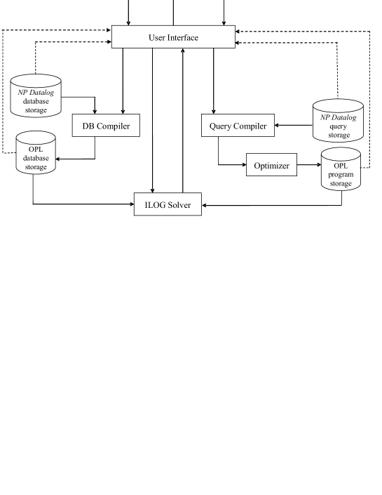
Figure 1: System Architecture.

• User Interface – This module receives in input a pair of strings identifying the file containing the source database and the file containing the query. If both the database and the query have already been translated, then the UI asks the module ILOG Solver to execute the query. If the database (resp. query) has not been translated, then the UI sends the name of the file containing the source database (resp. query) to the module Database Compiler (resp. Query Compiler) to be translated. Moreover, this module is in charge of visualizing the answer to the input query.

• Database compiler – This module translates the source database into an OPL database.

• Query compiler – This module receives in input an ${\mathcal{}N\!P\,D}atalog$ query and gives in output the corresponding OPL code. In order to check the correctness of the query and generate the target code, the module uses information on the schema of predicates.

• Optimizer – This module rewrites the OPL code received from the module Query Compiler and gives in output the target (optimized) OPL code.

• Query executor – This module consists of the ILOG OPL Development Studio which executes the query stored by the module Optimizer into the OPL program storage, over a database stored into the OPL database storage. The module Query executor interacts with the module User Interface by providing it the obtained result.

Therefore, ${\mathcal{}N\!P\,D}atalog$ can be also used to define a logic interface for constraint programming solvers such as ILOG. The experiments presented in this subsection show that the combination of the two components is effective so that constraint solvers (as well as SAT solvers) can be used as an efficient tool for computing logic queries whose semantics is based on stable models.

In order to assess the efficiency of our approach, we have performed several experiments comparing the performance obtained by implementing ${\mathcal{}N\!P\,D}atalog$ over the ILOG OPL Development Studio against Answer Set Programming systems. Specifically,  ${\mathcal{}N\!P\,D}atalog$/OPL  has been compared with DLV, Smodels, ASSAT, Clasp and XSB. The following version of the aforementioned systems have been used:

• ILOG OPL Development Studio 6.1 [ILOG OPL Studio]

• DLV release 2007-10-11 [DLV Web Site]

• Smodels 2.33 (and lparse 1.1.1) [Smodels Web Site]

• ASSAT 2.02 (lparse 1.1.1 and zChaff 2007.3.12) [ASSAT Web Site, zChaff]

• Clasp 1.2.1 (and lparse 1.1.1) [Clasp Web Site]

• XSB version 3.2 March 15, 2009 [XSB Web Site]

The performances of the systems have been evaluated by measuring the time necessary to find one solution of the following problems: 3-Coloring, Hamiltonian Cycle, Transitive Closure, Min Coloring, N-Queens and Latin Squares.

For each system, we have used efficient encodings of the problems which exploit efficient built-in constructs provided by the systems. Every encoding and database used in the experiments can be downloaded from the ${\mathcal{}N\!P\,D}atalog$ web site (http://wwwinfo.deis.unical.it/npdatalog/).

All the experiments were carried out on a PC with a processor Intel Core Duo 1.66 GHz and 1 GB of RAM under the Linux operating system . In the sequel of this section the experimental results are presented.

3 Coloring.

The 3-Coloring query has been evaluated on structured graphs of the form reported in Fig. 2(i) and random graphs. Specifically, structured graphs with $base\mathchar 61\relax height$ have been used (here $base$ denotes the number of nodes in the same row, $height$ the number of nodes in the same column; the total number of nodes in the graph is $base*height$). The random graphs have been generated by means of Culberson’s graph generator [K-Colorable graph generator]. Specifically, the following parameters have been used: K-coloring scheme equal to Equi-partitioned, Partion number equal to 3, Graph type is IID (independent random edge assignment). Both structured and random graphs are all 3-colorable; the results, showing the execution times (in seconds) as the size of the graph increases, are reported in Fig. 4 and Fig. 4, respectively.

(i)		(ii)

Figure 2: Structured Graphs.          

As for structured graphs, the $x$-axis reports the number of nodes in the same layer (i.e. the value of $base$). ${\mathcal{}N\!P\,D}atalog$ and DLV are faster than the other systems; ASSAT and Clasp have almost the same execution times (observe that the scale of the $y$-axis is logarithmic).

Regarding random graphs, it is worth noting that we have considered, for each number of nodes, five different graphs. Thus, the execution times reported in Fig. 4 have been obtained by evaluating the query five times (over different graphs with the same number of nodes) and computing the mean value. ${\mathcal{}N\!P\,D}atalog$/OPL is faster than the other systems; again, ASSAT and Clasp have almost the same execution times.

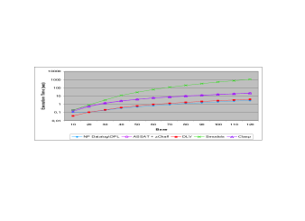
Figure 3: Execution time for the 3-coloring problem on structured graphs.

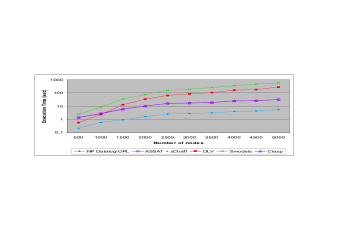
Figure 4: Execution time   for  the 3-coloring problem on random graphs.

Hamiltonian Cycle.

The Hamiltonian Cycle problem has been evaluated over benchmark graphs used to test other systems [HC Instances] and random graphs generated by means of Culberson’s graph generator [HC Program Archive]. All the graphs have a Hamiltonian cycle. The ${\mathcal{}N\!P\,D}atalog$ encoding (as well as the encodings for the other systems) can be found on [${\mathcal{}N\!P\,D}atalog$ Web site]. The results are reported in Fig. 6 and Fig. 6. The $x$-axis reports the used graphs: a label $nvXaY$ refers to a graph with $X$ nodes and $Y$ arcs. Observe that, in Fig. 6, a missing value means that the system has not answered in 30 minutes. Clasp is the fastest system for both types of graphs. DLV and Smodels are on average faster than the remaining systems. For large “dense” graphs Smodels outperforms DLV, but on some benchmark instances it runs out of time.

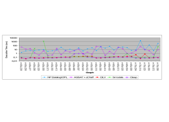
Figure 5: Execution time for the Hamiltonian Cycle problem on benchmark graphs.

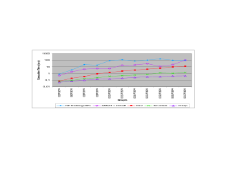
Figure 6: Execution time for the Hamiltonian Cycle problem on random graphs.

Transitive Closure.

The Transitive Closure problem has been evaluated over directed structured graphs such as those reported in Fig. 7. Specifically, instances with $base\mathchar 61\relax height$ have been used ($base$ denotes the number of nodes in the same row, $height$ the number of nodes in the same column).

Figure 7: Directed structured graphs.

The results, which are reported in Fig. 8, show that DLV and XSB are faster than the other systems; ASSAT, Clasp and Smodels almost have the same execution times.

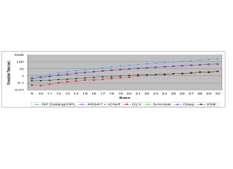
Figure 8: Execution time for the Transitive Closure problem on directed structured graphs.

Min Coloring.

As for the Min Coloring optimization problem, we have used structured graphs such as those of Fig. 2. Instances having the structure reported in Fig. 2(i) need at least three colors to be colored, whereas instances having the structure reported in Fig. 2(ii) need at least four colors to be colored. The number of colors available in the database has been fixed for the two structures, respectively, to four and five (one more than the number of colors necessary to color the graph). The results are reported in Fig. 9 and show that ${\mathcal{}N\!P\,D}atalog$ outperforms DLV. A missing time means that DLV runs out of time (also in this case we had a 30 minute time-limit).

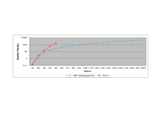
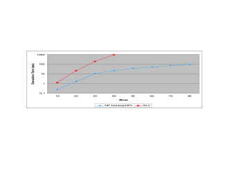
(i)		(ii)

Figure 9: Execution time for the Min Coloring problem on structured graphs.

N-Queens.

We have considered empty chessboards to be filled with $N$ Queens for increasing values of $N$. The results are reported in Fig. 10. Clasp is faster than ${\mathcal{}N\!P\,D}atalog$ which is in turn faster than ASSAT; for a high number of queens, DLV and Smodels become slower than the other systems.

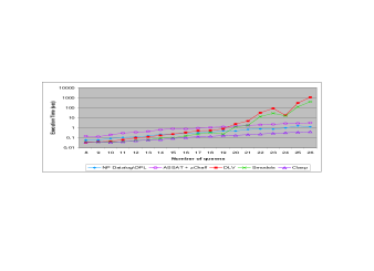
Figure 10: Execution time for the N-Queens problem.

Latin Squares.

We have considered partially filled tables which have been generated randomly. In every table, $60\%$ of the squares are empty. We have considered, for each table size, five different instances. Thus, the execution times reported in Fig. 11 have been obtained by evaluating the query five times (over different tables of the same size) and computing the mean value. The results show that ${\mathcal{}N\!P\,D}atalog$ and Clasp are faster than the other systems.

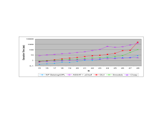
Figure 11: Execution time for the Latin Squares problem on random squares.

The experimental results reported above show that our system only seems to suffer with programs where the evaluation of the deterministic components is predominant. The reason is that deterministic components (often consisting of recursive rules) are translated into OPL scripts, which correspond to the evaluation of such components by means of the naive fixpoint algorithm, whereas problems which can be expressed without recursion (or in which the non-deterministic components are predominant) are executed efficiently. The implementation of our system prototype could be enhanced by making more efficient the translation of stratified (sub)programs or by using a different evaluator for these components. For instance, they could be evaluated by means of ASP systems, thus combining their efficiency in the computation of deterministic components with the efficiency of OPL in the computation of non-deterministic components.

6 Related Languages and Systems

Several languages have been proposed for solving $\mathcal{}N\!P$ problems. Here we have analyzed three different classes of languages: specification languages, constraint and logic programming languages, and answer set logic languages.

Specification Languages

Specification languages are highly declarative and allow the user to specify problems in terms of guess and check techniques.

NP-SPEC [Cadoli et al. 2000, Cadoli and Schaerf 2005] is a logic-based specification language allowing the built-in second-order predicates Subset, Partition, Permutation and IntFunc. The semantics of an NP-SPEC program is based on the notion of model minimality and the language upon which this semantics relies on is $DATALOG^{CIRC}$, i.e. an extension of DATALOG in which only some predicates are minimized and the interpretation of the other is left open. An NP-SPEC program consists of two sections: the DATABASE section, specifying the instance and the SPECIFICATION section specifying the question. To make NP-SPEC executable, specifications are translated into SAT instances and then executed using a SAT solver.

KIDS (Kestrel Interactive Development System) [Smith 1990] is a semi-automatic program development system that, starting from an initial specification of the problem, produces an executable code through a set of consistency-preserving transformations. The problem is written in a logic based language augmented with set-theoretic data types and functional constraints on the input/output behavior. To make the language executable, specifications are firstly translated into $CommonLisp$ and then into machine code. Before the compilation task, the user may select an optimization technique, such as simplification or partial evaluation, to obtain a more efficient target code.

SPILL-2 (SPecifications In a Logic Language) is the second version of an executable typed logic language that is an extension of the Prolog-like language Goedel [Kluzniak and Milkowska 1997]. A specification in SPILL-2 consists of a set of type declarations, a set of function declarations, a set of predicate declarations and a number of logical expressions (queries) that are used to test the specification. A specification in SPILL is required to be “executable” in the sense that it is possible to “test” whether a provided solution is feasible w.r.t. a given specification. The execution of a program consists in evaluating each query in the context of the specification and reporting the result (true if the query succeeds and false otherwise).

Constraint and Logic Programming Languages

The basic idea of constraint programming (CP) is to model and solve a problem by exploring the set of constraints that fully characterize the problem. Almost all computationally hard problems, such as planning, scheduling and graph theoretic problems, fall into this category. A large number of systems (more than 40) for solving CP problems have been developed in computer science and artificial intelligence:

• Constraint Logic Programming, an extension of logic programming able to manage constraints, started about 20 years ago by Jaffar et al. [Jaffar et al. 1992]. Several constraint logic languages allowing the formulation of constraints over different domains exist. Basically, all these languages embed efficient constraint solvers in logic based programming languages, such as Prolog. Here we cite, among the others, CLP [Marriott and Stuckey 1998], SICStus Prolog [SICStus Prolog Web Site], BProlog [Zhou 2002], ECLiPSe [Wallace and Schimpf 1999] and Mozart [Van Roy et al. 1999].

• ILOG OPL Development Studio [ILOG OPL Studio], an integrated development environment for mathematical programming and combinatorial optimization applications. The syntax of OPL is well-suited to express optimization problems defined in the mathematical programming style [Van Hentenryck 1988, Van Hentenryck et al. 1999].

• Constraint LINGO [Finkel et al. 2004], a high-level logic-programming language for expressing tabular constraint-satisfaction problems such as those found in logic puzzles and combinatorial problems such as graph coloring.

Several languages extending Prolog have been proposed as well. Most of these languages have been designed to provide powerful capabilities to represent and solve general problems and not to solve $\mathcal{}N\!P$ problems. Here we mention:

BinProlog [BinProlog], a fast and compact Prolog compiler, based on the transformation of Prolog to binary clauses. BinProlog is based on the BinWAM abstract machine, a specialization of the WAM for the efficient execution of binary logic programs.

XSB [Rao et al. 1997], an extension of Prolog supporting the well-founded semantics [Van Gelder et al. 2001] and including implementations of OLDT (tabling) and HiLog terms. OLDT resolution is extremely useful for recursive query computation, allowing programs to terminate correctly in many cases where Prolog does not. HiLog supports a type of higher-order programming in which predicate symbols can be variable or structured.

An extension of classical first order logic, called ID-Logic, has been proposed in [Denecker 2000]. Basically, in an ID-Logic theory, we can distinguish four different components describing i) data, ii) open predicates, iii) definitions and iv) assertions (or constraints). The relationships between ID-Logic and ASP has been studied in [Marien et al. 2004], where it has been also presented how ID-Logic theories can be translated into DATALOG^¬ programs under ASP semantics.

Answer Set Programming Languages and Systems

Several deductive systems based on stable model semantics have been developed too. Here we discuss some of the more interesting answer-set based systems and languages:

DLV (Vienna Univ. of Technology and University of Calabria) [Leone et al. 2006, Eiter et al. 1997] is a deductive database system, based on disjunctive logic programming. DLV extends Datalog with general negation, inclusive head disjunction and two different forms of constraints: strong constraints, which must be satisfied, and weak constraints, which are satisfied if possible (preferred models are those which minimize the number of ground weak constraints which are not satisfied). For instance, the program of Example 1 is a DLV program, whereas by replacing exclusive disjunction with inclusive disjunction in the program of Example 2 we get a DLV program (the minimality of the models guarantees that every node cannot belong to both relations $\mathtt{v}$ and $\mathtt{n}v$). The optimization query of examples 1 and 2 can be defined by adding the weak constraint $\mathtt{:}\sim v(X)$ which minimizes the number of ground false weak constraints (i.e. $\mathtt{v}$-tuples).

Smodels (Helsinki Univ. of Technology) [Simons et al. 2002] is a system for answer set programming consisting of Smodels, an efficient implementation of the stable model semantics for normal logic programs and lparse, a front-end that transforms user programs so that they can be understood by Smodels.

Besides standard rules lparse also supports a number of extended rules: choice, constraint and weight rules. The formal semantics of all three types of rules can be defined through the use of weight constraints and weight constraint rules. In lparse the weight constraints are implemented as special literal types. Basically, a weight constraint is of the form: $L\leq l_{1}\mathchar 61\relax w_{1},\dots,l_{n}\mathchar 61\relax w_{n}\leq U$ where $l_{1},\dots,l_{n},$ are literals, $L$ and $U$ are the integral lower and upper bounds, and $w_{1},\dots,w_{n}$ are weights of the literals. The intuitive semantics of a weight constraint is that it is satisfied exactly when the sum of weights of satisfied literals $l_{1},\dots,l_{n}$ is between $L$ and $U$, inclusive. A weight constraint rule is of the form $C_{0}\leftarrow C_{1},\dots,C_{n}$ where $C_{0},\ldots,C_{n}$ are weight constraints. Besides the use of literals, lparse also enhances the use of conditional literals having the form: $p(X):q(X)$ where $p(X)$ is any basic literal and $q(X)$ is a domain predicate.

Datalog Constraint. [East and Truszczynski 2000] proposed a new nonmonotonic logic, called Datalog with constraints or DC. A DC theory consists of constraints and Horn rules (Datalog program). The language is determined by a set of atoms $At\mathchar 61\relax At_{C}\cup At_{H}$ where $At_{C}$ and $At_{H}$ are disjoint. Formally, a DC theory is a triple $T\mathchar 61\relax(T_{C},T_{H},T_{PC})$ where $T_{C}$ is a set of constraints over $At_{C}$, $T_{H}$ is a set of Horn rules whose head atoms belong to $At_{H}$ and $T_{PC}$ is a set of constraints over $At$ (post constraints). The problem of the existence of an answer set, for a finite propositional $DC$ theory $T$, is $\mathcal{}N\!P$-complete [East and Truszczynski 2000].

ASSAT. [Lin and Zhao 2004] proposed a translation from normal logic programs with constraints under the answer set semantics to propositional logic. The peculiarity of this technique consists in the fact that for each loop in the program, a corresponding loop formula to the program’s completion is added. The result is a one-to-one correspondence between the answer sets of the program and the models of the resulting propositional theory. As in the worst case the number of loops in a logic program can be exponential, the technique proposes to add a few loop formulas at a time, selectively. Based on these results, a system called ASSAT(X), depending on the SAT solver X used, has been implemented for computing answer sets of a normal logic program with constraints.

Cmodels [Lierler 2005a, Lierler 2005b] is an answer set programming system that uses the frontend lparse and whose main computational characteristic is that it computes answer sets using a SAT solver for search. Cmodels deals with programs that may contain disjunctive, choice, cardinality and weight constraint rules. The basic execution steps of the system can be outlined as follows: (1) the program’s completion is produced; (2) a model of the completion is computed using a SAT solver; (3) if the model is indeed an answer set, then the model is returned, otherwise the system goes back to Step 2. The idea is thus to use a SAT solver for generating model candidates and then check if they are indeed the answer sets of a program. The way Step 3 is implemented depends on the class of a logic program.

Clasp [Gebser et al. 2007] is an answer set solver for (extended) normal logic programs. It combines the high-level modeling capacities of answer set programming (ASP) with state-of-the-art techniques from the area of Boolean constraint solving. In fact, the primary Clasp algorithm relies on conflict-driven learning, a technique that proved successful for satisfiability checking (SAT). Unlike other ASP solvers that use conflict-driven learning, Clasp does not rely on legacy software, such as a SAT solver or any other existing ASP solver.

A-Prolog [Gelfond 2002] is a logic language whose semantics is based on stable models, designed to represent defaults (i.e. statements of the form “Elements of a class $C$ normally satisfy property $P$”), exceptions and causal effects of actions (“statement $F$ becomes true as a result of performing an action $A$”). In the same work, an extension of the language, called ASET-Prolog, is presented. Such an extension enriches the language with two new types of atoms: s-atoms, which allows us to define subsets of relations, and f-atoms, which allows us to express constraints on the cardinality of sets. An interesting application showing how declarative programming in A-Prolog can be used to describe the dynamic behavior of digital circuits is presented in [Balduccini et al. 2000].

Comparison with the other approaches proposed in the literature

${\mathcal{}N\!P\,D}atalog$ is related i) to specification languages, for the style of defining problems, ii) to answer set languages, for the syntax and declarative semantics, and iii) to constraint programming.

Specification Languages

The problem with specification languages is the tradeoff between the expressiveness of the formal notation and its execution. In general, specifications can be executed only by blind search through the space of all proofs. A possible solution consists in adding (to specifications) refinements which improve the execution, but the result could be a longer specification, containing details and, consequently, hard to understand.

NP-SPEC programs have a structure similar to the one of ${\mathcal{}N\!P\,D}atalog$ programs, although from the syntax point of view, the use of meta-predicates, in some cases, does not make programs shorter and more intuitive (see, for instance, the N-Queen problem reported in [Cadoli and Schaerf 2005]). NP-SPEC uses in addition to standard Datalog rules, also meta-predicates and set operators, whereas ${\mathcal{}N\!P\,D}atalog$ uses only standard Datalog rules with shortcuts for limited forms of (unstratified) negation. Moreover, although there is no difference in expressivity, guesses in NP-SPEC are defined over base relations, whereas in ${\mathcal{}N\!P\,D}atalog$ they are defined over general ‘deterministic’ relations defined by stratified Datalog programs. As a further difference, the partition mechanism is more general and flexible in ${\mathcal{}N\!P\,D}atalog$ w.r.t. NP-SPEC as in the latter the number of partitions is fixed. Concerning the semantics aspects, the declarative semantics of NP-SPEC programs is based on the notion of model minimality, whereas those of ${\mathcal{}N\!P\,D}atalog$ is based on stable models.

KIDS results are “sensitive” to the implementation issue. Indeed, the KIDS system is semiautomatic: the user is asked to interact with the system in order to transform high level declarative specification into an efficient, correct and executable program. Moreover, the complexity of the final implementation in KIDS can result in dramatic improvements if specialized techniques are used. On the other hand, ${\mathcal{}N\!P\,D}atalog$ is a fully declarative language whose execution process is automatically optimized by the ILOG OPL Development Studio.

SPILL-2 is not meant to use the specification of a problem in order to compute a solution, but to test the specification against some specific case, i.e. to verify whether a given specification implies certain intended properties or, in other words, if a specified property is consistent with the specification. As for differences, specification and queries in SPILL are compiled to Prolog, whereas our approach introduces specifications using ${\mathcal{}N\!P\,D}atalog$ and then performs the translation of queries into OPL programs. Moreover, ${\mathcal{}N\!P\,D}atalog$ is based on stable model semantics, whereas SPILL uses a pure first order semantics, i.e. it does not include any form of model minimization operations. As for a further difference, it is worth noting that SPILL does not provide a characterization of its expressive power and its complexity.

Constraint and Logic Programming Languages

Constraint Logic Languages, such as SICStus Prolog, ECLiPSe and BProlog, are extensions of Prolog and, therefore, they are not fully-declarative. Their semantics is based on top-down evaluation of queries (SLDNF resolution), whereas answer-set programming is based on bottom-up evaluation. $XSB$ is an extension of Prolog with a declarative semantics (namely the well-founded semantics) based on top-down evaluation of queries (OLDT resolution) with tabling. Moreover, while answer-set languages permit $\mathcal{}N\!P$ problems to be easily expressed (it suffices to translate their logic definition into logic programming rules), constraint logic programming languages are procedural and the efficient implementation of $\mathcal{}N\!P$ problems is hard and time-consuming.

The relationship between ID Logic and ${\mathcal{}N\!P\,D}atalog$ is strong since in our language we can also distinguish components describing data, guess predicates, standard rules and constraints, which correspond, respectively, to the ID logic components describing data, open predicates, definitions and constraints. Moreover, the aim of ${\mathcal{}N\!P\,D}atalog$ is also the easy translation into different formalisms (other than ASP), including constraint programming languages.

Answer Set Programming Languages

The main difference of ${\mathcal{}N\!P\,D}atalog$ with respect to DLV and Smodels is that only restricted forms of (unstratified) negations, embedded into built-in constructs, are allowed. As a consequence, ${\mathcal{}N\!P\,D}atalog$ is less expressive than DLV since the latter also uses (inclusive) disjunction and permits expression of problems in the second level of the polynomial hierarchy. The use of simpler languages such as ${\mathcal{}N\!P\,D}atalog$ allows us to avoid writing non-intuitive queries which are difficult to optimize or translate in other formalisms for which efficient executors exist. It is important to observe that cardinality constraints and conditional literals of Smodels allows us to express both subset and (generalized) partition rules as defined in ${\mathcal{}N\!P\,D}atalog$. This means that in Smodels it is also possible to avoid using unstratified negation without losing expressiveness. We also note that s-atoms and f-atoms of ASET-Prolog enable us to express subset and (generalized) partition rules.

${\mathcal{}N\!P\,D}atalog$ is also strongly connected to Datalog Constraint (DC), which is also based on stable model semantics. The main difference between ${\mathcal{}N\!P\,D}atalog$ and DC consists in the fact that ${\mathcal{}N\!P\,D}atalog$ forces users to write queries in a more disciplined form. In particular, DC guesses are expressed by means of constraints (a guess is any set of atoms in $At_{C}$ satisfying the constraint in $T_{C}$) and there is no clear separation between $T_{C}$ (constraints used to guess) and $T_{PC}$ (constraints used to check). Moreover, DC only uses positive rules to infer true atoms, whereas ${\mathcal{}N\!P\,D}atalog$ uses stratified rules. The expressive power of both languages captures the first level of the polynomial hierarchy. The experiments reported in [East and Truszczynski 2000] show that the guess and check style of expressing hard problems can be further optimized.

The philosophy of ASSAT is similar to that of ${\mathcal{}N\!P\,D}atalog$: while in the ASSAT approach programs are translated in propositional logic and then executed by means of a SAT solver, ${\mathcal{}N\!P\,D}atalog$ programs are translated into OPL programs and then executed by using the ILOG OPL Development Studio. An approach similar to the one of ASSAT is adopted by Cmodels.

A-Prolog is a general logic language (i.e. it allows function symbols, classical negation, head disjunction and subset rules) whose semantics is based on stable models. The aim of A-Prolog is the design of a general language for knowledge representation and causal reasoning, whereas ${\mathcal{}N\!P\,D}atalog$ is a simpler language (similar to the restricted FA-Prolog) which can be easily efficiently executed and translated in other formalisms.

7 Conclusion

$\mathcal{}N\!P$ search and optimization problems can be formulated as DATALOG^¬ queries under non-deterministic stable model semantics. In order to enable a simpler and more intuitive formulation of these problems, the ${\mathcal{}N\!P\,D}atalog$ language has been proposed. It is obtained by extending stratified Datalog with constraints and two constructs for expressing partitions of relations, so that search and optimization queries can be expressed using only simple forms of unstratified negation. It has also been shown that ${\mathcal{}N\!P\,D}atalog$ captures the class of $\mathcal{}N\!P$ search and optimization problems and that ${\mathcal{}N\!P\,D}atalog$ queries can be easily translated into OPL programs. An algorithm for the translation of ${\mathcal{}N\!P\,D}atalog$ programs into OPL statements has been provided and its correctness has been proved. The proposed algorithm has been implemented by a system prototype which takes in input an ${\mathcal{}N\!P\,D}atalog$ query and gives in output an equivalent OPL program which is then executed using the ILOG OPL Development Studio. Consequently, ${\mathcal{}N\!P\,D}atalog$ can also be used to define a logic interface for constraint programming solvers. Several experiments comparing the computation of queries by different systems have shown the validity of our approach.

References

- 1
- Abiteboul et al. 1995 Abiteboul, S., Hull, R., and Vianu, V. 1995. Foundations of Databases. Addison-Wesley.
- ASSAT Web Site ASSAT Web Site. http://assat.cs.ust.hk/
- Balduccini et al. 2000 Balduccini, M., Gelfond, M., and Nogueira, M. 2000. A-Prolog as a tool for declarative programming. International Conference on Software Engineering and Knowledge Engineering, 63–72.
- Baral 2003 Baral, C. 2003. Knowledge Representation Reasoning and Declarative Problem Solving. Cambridge University Press.
- BinProlog BinProlog. http://www.binnetcorp.com/BinProlog/
- Cadoli and Schaerf 2005 Cadoli, M. and Schaerf, A. 2005. Compiling problem specifications into SAT. Artificial Intelligence, 162(1–2), 89–120.
- Cadoli et al. 2000 Cadoli, M., Ianni, G., Palopoli, L., Schaerf, A., and Vasile, D. 2000. NP-SPEC: An Executable Specification Language for Solving All Problems in NP. Computer Languages, 26(2–4), 165–195.
- Cholewinski et al. 1996 Cholewinski, P., Marek, V. W., and Truszczynski, M. 1996. Default Reasoning System DeReS. Proceedings of the International Conference on Principles of Knowledge Representation and Reasoning, 518–528.
- Clasp Web Site Clasp Web Site. http://www.cs.uni-potsdam.de/clasp/
- Denecker 2000 Denecker, M. 2000. Extending Classical Logic with Inductive Definitions. Computational Logic, 703–717.
- DLV Web Site DLV Web Site. http://www.dbai.tuwien.ac.at/proj/dlv/
- East and Truszczynski 2000 East, D. and Truszczynski, M. 2000. DATALOG with Constraints - An Answer-Set Programming System. Proceedings of the National Conference on Artificial Intelligence, 163–168.
- East and Truszczynski 2006 East, D. and Truszczynski, M. 2006. Predicate-calculus based logics for modeling and solving search problems. ACM Transaction on Computational Logic, 7(1), 38–83.
- Eiter et al. 1997 Eiter, T., Leone, N., Mateis, C., Pfeifer G., and Scarcello, F. 1997. A Deductive System for Non-monotonic Reasoning. Proceedings of the International Conference on Logic Programming and Nonmonotonic Reasoning, 363–374.
- Fagin 1974 Fagin, R. 1974. Generalized First-Order Spectra and Polynomial-Time Recognizable Sets. In Complexity of Computation (R. Karp, Ed.), SIAM-AMS Proc., Vol. 7, 43–73.
- Finkel et al. 2004 Finkel,R. A., Marek, V. W., and Truszczynski, M. 2004. Constraint Lingo: towards high-level constraint programming. Software Practice and Experience, 34(15), 1481-1504.
- Gebser et al. 2007 Gebser, M., Kaufmann, B., Neumann, A., and Schaub, T. 2007. Conflict-Driven Answer Set Solving. Twentieth International Joint Conference on Artificial Intelligence.
- Gelfond and Lifschitz 1988 Gelfond, M. and Lifschitz, V. 1988. The Stable Model Semantics for Logic Programming. Proceedings of the International Conference on Logic Programming, 1070–1080.
- Gelfond 2002 Gelfond, M. 2002. Representing Knowledge in A-Prolog. Computational Logic: Logic Programming and Beyond, 413–451.
- Greco 1999 Greco, S. 1999. Dynamic Programming in Datalog with Aggregates. IEEE Transactions on Knowledge and Data Engineering, 11(2), 265–283.
- Greco and Saccà 2002 Greco, S. and Saccà, D. 2002. Search and Optimization Problems in Datalog. Computational Logic: Logic Programming and Beyond, 61–82.
- Greco and Saccà 1997 Greco, S. and Saccà, D. 1997. NP Optimization Problems in Datalog. Symposium on Logic Programming, 181–195.
- Greco et al. 1995 Greco, S., Saccà, D., and Zaniolo C. 1995. Datalog with Stratified Negation and Choice: from to . Proceedings of the International Conference on Database Theory, 574–589.
- Greco and Zaniolo 2001 Greco, S. and Zaniolo, C. 2001. Greedy Algorithms in Datalog. Theory and Practice of Logic Programming, 1(4), 381–407.
-
HC Program Archive
Hamiltonian Cycle Program Archive.
http://web.cs.ualberta.ca/joe/Theses/HCarchive/main.html - HC Instances Hamiltonian Cycle Instances. http://assat.cs.ust.hk/Assat-2.0/hc-2.0.html
- ILOG OPL Studio ILOG OPL Studio. http://www.ilog.com/products/oplstudio/
- Jaffar et al. 1992 Jaffar, J., Michaylov, S., Stuckey, P.J., and Yap, R. 1992. The CLP(R) Language and System. ACM Transaction on Programming Languages and Systems, 14(3), 339–395.
- Johnson 1990 Johnson, D. S. 1990. A Catalog of Complexity Classes. In Handbook of Theoretical Computer Science, Vol. 1, J. van Leewen (ed.), North-Holland, 67– 161.
-
K-Colorable graph generator
K-Colorable graph generator.
http://web.cs.ualberta.ca/joe/Coloring/Generators/generate.html - Kluzniak and Milkowska 1997 Kluzniak, F. and Milkowska, M. 1997. Spill - A Logic Language for Writing Testable Requirements Specifications. Science of Computer Programming, 28(2-3), 193–223.
- Kolaitis and Papadimitriou 1991 Kolaitis, P. and Papadimitriou, C. 1991. Why not Negation by Fixpoint? Journal of Computer and System Sciences, 43(1), 125–144.
- Kolaitis and Thakur 1995 Kolaitis, P. G. and Thakur, M. N. 1995. Approximation Properties of NP Minimization Classes. Journal of Computer and System Sciences, 51, 391–411.
- Leone et al. 2006 Leone, N., Pfeifer, G., Faber, W., Eiter, T., Gottlob, G., Perri, S., and Scarcello, F. 2006. The DLV System for Knowledge Representation and Reasoning. ACM Transactions on Computational Logics, 7(3), 499–562.
- Lierler 2005a Lierler, Y. 2005. Disjunctive Answer Set Programming via Satisfiability. Answer Set Programming.
- Lierler 2005b Lierler, Y. 2005. Cmodels - SAT-Based Disjunctive Answer Set Solver. Logic Programming and Nonmonotonic Reasoning, 447–451.
- Lin and Zhao 2004 Lin, F. and Zhao, Y. 2004. ASSAT: computing answer sets of a logic program by SAT solvers. Artificial Intelligence 157(1-2), 115–137.
- Marek and Truszczynski 1991 Marek, W. and Truszczynski, M. 1991. Autoepistemic Logic. Journal of the ACM, 38(3), 588–619.
- Marien et al. 2004 Marien, M., Gilis, D., and Denecker, M. 2004. On the Relation Between ID-Logic and Answer Set Programming. Logics in Artificial Intelligence, 108–120.
- Marriott and Stuckey 1998 Marriott, K. and Stuckey, P. J. 1998. Programming with Constraints: An Introduction. MIT Press.
- Niemela et al. 1999 Niemela, I., Simons, P., and Soininen, T. 1999. Stable Model Semantics of Weight Constraint Rules. Proceedings of the International Conference on Logic Programming and Nonmonotonic Reasoning, 317–331.
- Web site NP Datalog Web site. http://wwwinfo.deis.unical.it/npdatalog/
- Papadimitriou and Steiglitz 1982 Papadimitriou, C. H. and Steiglitz, K. 1982. Combinatorial Optimization—Algorithms and Complexity. Prentice-Hall.
- Papadimitriou and Yannakakis 1982 Papadimitriou, C. H. and Yannakakis, M. 1982. Optimization, Approximation, and Complexity Classes. Journal Computer and System Sciences, 43, 425–440.
- Papadimitriou 1994 Papadimitriou, C. H. 1994. Computational Complexity. Addison-Wesley.
- Rao et al. 1997 Rao, P., Sagonas, K.F., Swift, T., Warren, D.S., and Freire, J. 1997. XSB: A System for Effciently Computing WFS. Proceedings of the International Conference on Logic Programming and Nonmonotonic Reasoning, 431–441.
- Saccà 1997 Saccà, D. 1997. The Expressive Powers of Stable Models for Bound and Unbound Queries. Journal of Computer and System Sciences, 54(3), 441–464.
- Schlipf 1995 Schlipf, J. S. 1995. The Expressive Powers of the Logic Programming Semantics. Journal of Computer and System Sciences, 51(1), 64–86.
- Smith 1990 Smith, D. R. 1990. KIDS: A Semiautomatic Program Development System. IEEE Transaction on Software Engineering, 16(9), 1024–1043.
- SICStus Prolog Web Site SICStus Prolog Web Site. http://www.sics.se/isl/sicstuswww/site/index.html
- Simons et al. 2002 Simons, P., Niemela, I. and Soininen, T. 2002. Extending and Implementing the Stable Model Semantics. Artificial Intelligence, 138(1-2), 181-234.
- Smodels Web Site Smodels Web Site. http://www.tcs.hut.fi/Software/smodels/
- Ullman 1988 Ullman, J. K. 1988. Principles of Data and Knowledge-Base Systems, Vol. 1 and 2. Computer Science Press, New York.
- Van Gelder et al. 2001 Van Gelder, A., Ross, K.A., and Schlipf, J.S. 2001. The Well-Founded Semantics for General Logic Programs. Journal of ACM, 620–650.
- Van Hentenryck 1988 Van Hentenryck, P. 1988. The OPL Optimization Programming Language. Mit Press.
- Van Hentenryck et al. 1999 Van Hentenryck, P., Michel, L., Perron, L., and Regin, J. C. 1999. Constraint Programming in OPL. Proceedings of the International Conference on Principles and Practice of Declarative Programming, 98–116.
- Van Roy et al. 1999 Van Roy, P. 1999. Logic Programming in Oz with Mozart. Proceedings of the International Conference on Logic Programming, 38–51.
- Wallace and Schimpf 1999 Wallace, M. and Schimpf, J. 1999. ECLiPSe: Declarative Specification and Scaleable Implementation. Proceedings of the International Workshop on Practical Aspects of Declarative Languages, 365–366.
- XSB Web Site XSB Web Site. http://xsb.sourceforge.net/
- zChaff zChaff. http://www.princeton.edu/chaff/zchaff.html
- Zhou 2002 Zhou, N. 2002. Implementing Constrant Solvers in B-Prolog. Intelligent Information Processing, 249-260.
- Zumpano et al. 2004 Zumpano, E., Greco, S., Trubitsyna, I., and Veltri, P. 2004. On the semantics and expressive power of Datalog-like languages for NP search and optimization problems. Proceedings of the ACM Symppsium on Applied Computing, 692–697.