Spatial Analysis of Opportunistic Downlink Relaying in a Two-Hop Cellular System

Abstract

We consider a two-hop cellular system in which the mobile nodes help the base station by relaying information to the dead spots. While two-hop cellular schemes have been analyzed previously, the distribution of the node locations has not been explicitly taken into account. In this paper, we model the node locations of the base stations and the mobile stations as a point process on the plane and then analyze the performance of two different two-hop schemes in the downlink. In one scheme the node nearest to the destination that has decoded information from the base station in the first hop is used as the relay. In the second scheme the node with the best channel to the relay that received information in the first hop acts as a relay. In both these schemes we obtain the success probability of the two hop scheme, accounting for the interference from all other cells. We use tools from stochastic geometry and point process theory to analyze the two hop schemes. Besides the results obtained a main contribution of the paper is to introduce a mathematical framework that can be used to analyze arbitrary relaying schemes. Some of the main contributions of this paper are the analytical techniques introduced for the inclusion of the spatial locations of the nodes into the mathematical analysis.

I Introduction

Cellular systems are the most widely deployed wireless systems and provide reliable communication services to billions around the world. They consist of base stations that serve a geographical area called cell. In most of the present cellular systems, the base station (BS) communicates directly with the mobile users (MS) in its cell. This single-hop architecture makes it is difficult for the BSs to communicate with MSs at the cell boundary because of the distance and the inter-cell interference. So a base station will have to increase its power to maintain the rate of transmission. The dead spots problem can be countered by using more base stations, thereby increasing the spatial reuse. But increasing the number of base stations can be prohibitively expensive or even impossible. The problem can be addressed more effectively by moving away from the paradigm of single-hop communication and permitting the base station to communicate with mobile stations at the boundary by using the other intermediate MSs in its cell in a sequence of hops. Although such multi-hopping requires some significant changes in the present cellular system architecture, it may help to effectively combat the dead spots problem, and hence the cellular multi-hopping problem is worthy to investigate [1, 2]. In this paper, we analyze the benefits of two-hop cellular communication by comparing its performance with a traditional single-hop cellular system. A two-hop system,

• may provide significant benefits over single-hop communication.

• does not have the implementation complexity of larger number of hops (in terms of routing and scheduling).

When a BS transmits, multiple MSs will be able to receive the information, and hence these mobile nodes can help the BS transmit information to the cell edge. Since more than one MS can act as a relay, it is not clear how to choose a subset of these relays in a distributed fashion so as to reduce the interference and increase the probability of packet delivery. In this paper, we analyze simple relay selection schemes and compare their performance with direct transmission. We account for the inter-cell interference and the spatial structure of the transmitting nodes in the analysis.

We use methods from stochastic geometry and point process theory to model and study the two-hop cellular system. In particular we provide techniques based on probability generating functional of a point process to analyze the outage probabilities, and we provide asymptotic results for the outage at high $\mathsf{SNR}$ and low BS density. The techniques presented in this paper can be extended to analyze more complicated relay selection schemes, power control mechanisms and other multi-hop techniques. The major emphasis of the paper is in the methodology and the techniques of the analysis rather than the specifics of the communication system. For example we concentrate only on two specific relay selection methods although many more methods have been proposed in the literature.

I-A Previous work

The problem of two-hop extensions of cellular system has been studied extensively, and a provision for a multi-hop technique has been included in the A-GSM standard [1, 2]. In [3], a MS is selected to help the BS depending on the large-scale path-loss on the BS-relay link and the relay-destination link. [4] considers a similar problem, but the MSs that can act as relays are assumed to be located on a circle around the BS, and the authors provide various power allocation schemes and verify their performance by simulations. The present problem is also very similar to the problem of opportunistic relay selection. In [5, 6] a detailed analysis of a opportunistic two-hop relaying scheme obtaining full diversity order using distributed space-time codes has been provided. But a distributed space-time code requires very tight coordination and precise signaling among the relays, which increases the overhead and complexity in the system. An alternative approach is to choose the best relay, and in opportunistic relaying (OR) [7] a relay is chosen so as to maximize the minimum signal-to-noise ratio ($\mathsf{SNR}$) of the source-relay and the relay-destination links. In selection cooperation (SC)[8, 9] the relay with maximum relay-destination $\mathsf{SNR}$ is chosen and has been shown that SC and OR provide a similar diversity order. In [5, 7, 8, 9], distributed relay selection schemes are analyzed and asymptotes of the outage are provided for high $\mathsf{SNR}$. The asymptotes provided are functions of the means of fading coefficients between the source, relays and the destination. Averaging these results with respect to the spatial distribution of the nodes is difficult and hence we use an alternative approach. In our approach we model the node locations in a statistical manner and incorporate this information in the analysis from the start rather than averaging over the spatial locations at the end. Our emphasis is on low-overhead schemes that can readily be implemented.

The paper is organized as follows: In Section II the system model is introduced, assumptions stated and the metrics used in the paper defined. In Section III the outage probability in the direct connection between the BS and its destination is derived. In Sections IV and V the outage probability of the two-hop schemes employing different relay selection schemes are analyzed. The asymptotic gain of using the two-hop schemes over the direct connection is also studied in these sections. In Section VI simulation results are provided and compared to the theory.

II System Model

We assume that the BSs (cell towers) are arranged on a square lattice of density $\lambda_{b}$.

$$\Phi_{b}={\left\{\frac{x}{\sqrt{\lambda_{b}}},\quad x\in\mathbb{Z}^{2}\right\}}.$$

The analysis in this paper generalizes in a straightforward manner to any deterministic arrangement of BS. We assume that $n_{x}$ MSs are available to assist a BS $x\in\Phi_{b}$. More precisely, the locations of the mobile stations that assist the base station $x$ form a Poisson point process [10] (PPP) $\Phi_{x}$ of density $\lambda_{x}(y)=\eta(y-x)$. For example choosing $\eta(y)=\mathbf{1}_{y}([-1/2,1/2]^{2})$ and $\lambda_{b}=1$ would lead to a square coverage area for each base station. We use $\mathbf{1}_{x}(A)$ to denote the indicator function of set $A$. See Figure 1. Observe that it is not necessary for a MS to be associated to its nearest BS, i.e., some MSs may be outside the Voronoi cell of their BS. We further make the following assumptions:

1. The average number of MS that each BS serves is finite, i.e.,

   $$N=\int_{\mathbb{R}^{2}}\eta(x)\mathrm{d}x<\infty.$$

   This assumption implies that $\Phi_{x}$ cannot be homogeneous [10, 11].

2. The locations of the mobile users associated with different base stations are independent.

Since the number of MSs in each cell is Poisson with mean $N=\mathbb{E}[n_{x}]$, each cell is empty with probability $\exp(-N)$. We shall use $\mu$ to denote the probability that a cell is not empty, i.e., $\mu=1-\exp(-N)$.

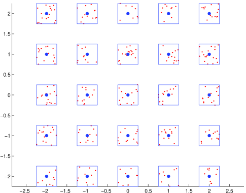
Figure 1: Illustration of the cellular system with $\lambda_{b}=1$ and $\eta(y)=50\cdot\mathbf{1}_{y}([-0.25,0.25]^{2})$. So on a average there are $12.5$ MSs per cell. The bold dots represent the BSs and the smaller dots the MSs. The white spaces between the cells may consist of other cells which transmit at a different frequency. We may model the case where the neighboring cells use the same frequency by choosing $\eta(y)=\mathbf{1}_{y}([-0.5,0.5]^{2})$.

Independent Rayleigh fading is assumed between any pair of nodes and also across time, and the power fading coefficient between a node $x$ and node $y$ is denoted by $\mathsf{h}_{xy}$. Hence $\mathsf{h}_{xy}$ is an exponential random variable with unit mean. The path-loss model is denoted by $\ell(x):\ \mathbb{R}^{2}\setminus\{o\}\rightarrow\mathbb{R}^{+}$ and is a continuous, positive, non-increasing function of $\|x\|$ that satisfies

$$\int_{\mathbb{R}^{2}\setminus B(o,\epsilon)}\ell(x)\mathrm{d}x<\infty,\quad\forall\epsilon>0,$$ (1)

where $B(a,r)$ denotes a disc of radius $r$ centered around $a$. $\ell(x)$ is usually taken to be a power law in one of the forms:

1. Singular path-loss model: $\|x\|^{-\alpha}$.

2. Non-singular path-loss model: $(1+\|x\|^{\alpha})^{-1}$ or $\min\{1,\|x\|^{-\alpha}\}$.

The integrability condition (1) requires $\alpha>2$ in all the above models. Assuming simple linear receivers and treating interference as noise, the communication between $x$ and $y$ is successful if

$$\mathsf{SINR}(x,y,\Phi)=\frac{p_{x}\mathsf{h}_{xy}\ell(x-y)}{\sigma^{2}+\sum_{z\in\Phi}p_{z}\mathsf{h}_{zy}\ell(z-y)}>\theta.$$ (2)

We also assume $\theta>1$ which implies at most one transmitter can connect to a receiver. Here $\Phi$ is the set of interfering transmitters, $p_{z}$ is the transmission power used by a transmitter located at $z$ and $\sigma^{2}$ is the the additive white Gaussian noise power at the receiver. We make the following assumptions:

1. In the two-hop schemes that will be analyzed, BSs transmit in the even time slots and the MSs transmit in the odd time slots, synchronized across all cells.

2. Each base station $x$ has an additional mobile station, the destination at $r(x)$ with $\|r(x)-x\|=R$, to which the BS wants to transmit information. This additional node just receives and never transmits.

3. All the BSs transmit with equal power $P$.

Notation:

• Define

  $$\mathbf{1}(x\rightarrow y\mid\Phi)=\mathbf{1}(\mathsf{SINR}(x,y,\Phi)>\theta).$$

  $\mathbf{1}(x\rightarrow y\mid\Phi)$ is the indicator random variable that is equal to one if a transmitter at $x$ is able to connect to a receiver $y$ when the interfering set is $\Phi$.

• Define

  $$\hat{\Phi}(x)=\left\{y\in\Phi_{x}:\ \mathbf{1}(x\rightarrow y\mid\Phi_{b}\setminus\{x\})\right\}.$$

  $\hat{\Phi}(x)$ is the set of MSs in the cell of BS $x$ to which the BS $x$ is able to connect in the first hop (even time slots).

Metric: Let $\mathsf{P}_{d}$ denote the probability that a BS can connect to its destination directly in the first hop. Since all BSs are identical

$$\mathsf{P}_{d}=\mathbb{E}\mathbf{1}(o\rightarrow r(o)\mid\Phi_{b}\setminus\{o\}).$$ (3)

where $o$ denotes the origin $(0,0)$. A BS can connect to multiple MSs in its cell, and these connected MS are the potential transmitters in the second hop. In the relay selection methods studied in the next section, a subset of these potential transmitters $R_{x}\subseteq\hat{\Phi}(x)$ are selected for each $x\in\Phi_{b}$ to transmit in the next hop. Let the probability that a relay can connect to its intended destination (determined by the source to which it connects in the first hop) in the second hop be $\mathsf{P}_{r}$, i.e.,

$$\mathsf{P}_{r}=1-\mathbb{E}\prod_{\mathsf{x}\in R_{o}}1-\mathbf{1}(\mathsf{x}\rightarrow r(o)\mid\Psi\setminus\{\mathsf{x}\}),$$ (4)

where $\Psi=\bigcup_{x\in\Phi_{B}}R_{x}$ is the set of all transmitters in the second hop. Here we are assuming no cooperative communication between nodes which have the same information, and hence relays belonging to the same cluster also interfere with each other in the second hop. Since $\theta>1$, at most one transmitter can connect to a receiver and thus

$$\mathsf{P}_{r}=\mathbb{E}\sum_{\mathsf{x}\in R_{o}}\mathbf{1}(\mathsf{x}\rightarrow r(o)\mid\Psi\setminus\{\mathsf{x}\}),$$ (5)

and the probability of success for the two-hop scheme is

$$\mathsf{P}_{s}=1-(1-\mathsf{P}_{d})(1-\mathsf{P}_{r}).$$

The BS can potentially transmit in the second hop instead of using the MS as intermediate relays. This retransmission scheme will be used as the base reference, and the performance of the relay selection schemes will be compared with this retransmission scheme. The gain in using the two-hop scheme over the retransmission scheme can be characterized as

$$\mathsf{G}(\mathsf{SNR},\lambda_{b})=\frac{(1-\mathsf{P}_{d})^{2}}{(1-\mathsf{P}_{d})(1-\mathsf{P}_{r})}=\frac{1-\mathsf{P}_{d}}{1-\mathsf{P}_{r}},$$ (6)

where

$$\mathsf{SNR}=\frac{P\ell(R)}{\sigma^{2}}$$

is the received SNR for the direct transmission. To compare the direct transmission with the relay selection scheme, power is allocated across the selected relays in the second hop so that the total power is equal to $P$. Another pertinent metric to capture the performance of the network is the diversity gain, defined as

$$\mathrm{d}(\lambda_{b})=-\lim_{\mathsf{SNR}\rightarrow\infty}\frac{\log(1-\mathsf{P}_{s})}{\log(\mathsf{SNR})}.$$

From the definition of the diversity and the gain, the following relation follows:

$$\mathrm{d}_{2}(\lambda_{b})-\mathrm{d}_{d}(\lambda_{b})=\lim_{\mathsf{SNR}\rightarrow\infty}\frac{\log(\mathsf{G}(\mathsf{SNR},\lambda_{b}))}{\log(\mathsf{SNR})},$$

where $\mathrm{d}_{d}$ is the diversity gain for the single-hop retransmission scheme, and $\mathrm{d}_{2}$ is the diversity gain of the two-hop scheme. From the definition of $\mathsf{P}_{s}$ it can be observed that the information received in the two time slots is decoded independently.

In the next sections, we will analyze the success probability $\mathsf{P}_{r}$ and the diversity order of the relay selection schemes. It is easy to observe that the probability $\mathsf{P}_{r}$ of any relay selection scheme does not tend to one by increasing the $\mathsf{SNR}$ because of the interference caused by transmissions in other cells. So to evaluate the asymptotic performance of the system, we scale the BS density as

$$\lambda_{b}=\mathsf{SNR}^{-\beta},\quad\beta\geq 0.$$ (7)

As will be evident in the next section, if the signal-to-interference ratio is defined as

$$\mathsf{SIR}=\frac{\ell(R)}{\sum_{\mathsf{x}\in\Phi_{b}\setminus\{o\}}\ell(\mathsf{x}-r(o))},$$ (8)

the scaling in (7) translates to

$$\mathsf{SIR}=\Theta(\mathsf{SNR}^{\frac{\alpha\beta}{2}}).$$

So the system is interference-limited when $\beta<2/\alpha$ and noise-limited otherwise. Hence the scaling in (7) helps us evaluate the performance of the system by varying $\beta$. In practice this scaling can be achieved by frequency planning and decreasing the spatial resuse factor. We now begin with the analysis of the direct transmission scheme.

III First Hop: Base Station Transmits

III-A Direct Connection

When the BSs transmit, the inter-cell interference, fading and the noise may cause the transmission to fail. The probability of direct connection is given by

$$\mathsf{P}_{d} = \mathbb{E}\mathbf{1}(o\rightarrow r(o)\mid\Phi_{b}\setminus\{o\})$$

$$= \mathbb{P}\left(\frac{\mathsf{h}_{xy}\ell(R)}{\frac{\sigma^{2}}{P}+\sum_{y\in\Phi_{B}\setminus\{o\}}\mathsf{h}_{yr(o)}\ell(y-r(o))}>\theta\right)$$

$$= \exp\left(-\frac{\theta\sigma^{2}}{P\ell(R)}\right)\prod_{y\in\Phi_{b}\setminus\{o\}}\frac{1}{1+\frac{\theta}{\ell(R)}\ell(y-r(o))}$$

$$= \exp\left(-\frac{\theta}{\mathsf{SNR}}\right)\Delta(r(o)),$$ (10)

where

$$\Delta(x)=\prod_{y\in\Phi_{b}\setminus\{o\}}\frac{1}{1+\frac{\theta}{\ell(x)}\ell(y-x)}.$$

The following lemma is required to analyze the asymptotics of the success probability.

Lemma 1

When $\ell(x)=\|x\|^{-\alpha}$ or $\ell(x)=1/(1+\|x\|^{\alpha})$,

$$\lim_{\lambda_{b}\rightarrow 0}\frac{1-\Delta(x)}{\lambda_{b}^{\alpha/2}}=\frac{\theta C(\alpha)}{\ell(x)},$$

where

$$C(\alpha)=\frac{\xi(\alpha/2,0)\left[\xi(\alpha/2,1/4)-\xi(\alpha/2,3/4)\right]}{2^{\alpha-2}}.$$ (11)

$\xi(s,b)=\sum_{k=0,k\neq-b}^{\infty}(k+b)^{-s}$ is the generalized Riemann zeta function.

Proof:

We consider the case of $\ell(x)=\|x\|^{-\alpha}$; the other case follows similarly. From the definition of $\Delta(x)$ it follows that

$$\exp\Big{(}-\theta\ell(x)^{-1}\sum_{y\in\Phi_{b}\setminus\{o\}}\ell(y-x)\Big{)} \leq \Delta(x)\leq\Big{(}1+\theta\ell(x)^{-1}\sum_{y\in\Phi_{b}\setminus\{o\}}\ell(y-x)\Big{)}^{-1}.$$

We have

$$\sum_{y\in\Phi_{b}\setminus\{o\}}\ell(y-x) = \sum_{y\in\mathbb{Z}^{2}\setminus\{o\}}\ell\left(\frac{y}{\sqrt{\lambda_{b}}}-x\right)$$

$$= \lambda_{b}^{\alpha/2}\sum_{y\in\mathbb{Z}^{2}\setminus\{o\}}\ell(y-x\sqrt{\lambda_{b}}).$$

Dividing both sides by $\lambda^{\alpha/2}$ and taking the limit, the result follows from the definition of the Epstein zeta function [12]. ∎

We have $C(3)\approx 9.03362$ and $C(4)\approx 6.02681$. From the derivation of the above lemma we observe that $\mathsf{SIR}\sim\mathsf{SNR}^{\alpha\beta/2}\ell(R)C(\alpha)^{-1}$ where the definition of $\mathsf{SIR}$ is provided in (8). Using the above lemma, the asymptotic expansion of $\mathsf{P}_{d}$ for $\lambda_{b}=\mathsf{SNR}^{-\beta},\beta\neq 0$, at high $\mathsf{SNR}$ is

$$\mathsf{P}_{d}\sim\left\{\begin{array}[]{ll}1-\theta\mathsf{SNR}^{-1}&\alpha\beta>2\\ 1-\theta\left(1+C(\alpha)\ell(R)^{-1}\right)\mathsf{SNR}^{-1}&\alpha\beta=2\\ 1-\theta C(\alpha)\ell(R)^{-1}\mathsf{SNR}^{-\alpha\beta/2}&0<\alpha\beta<2,\\ \end{array}\right.$$ (12)

and the diversity gain of the direct transmission is

$$\mathrm{d}_{d}(\mathsf{SNR}^{-\beta})=\min\left\{1,\frac{\beta\alpha}{2}\right\}.$$

So for the direct transmission, $\beta<2/\alpha$ corresponds to the interference-limited regime and $\beta>2/\alpha$ corresponds to the noise-limited regime. From Figure 2 we note that the asymptotes in (12) are close to the true $1-\mathsf{P}_{r}$ even at moderate $\mathsf{SNR}$.

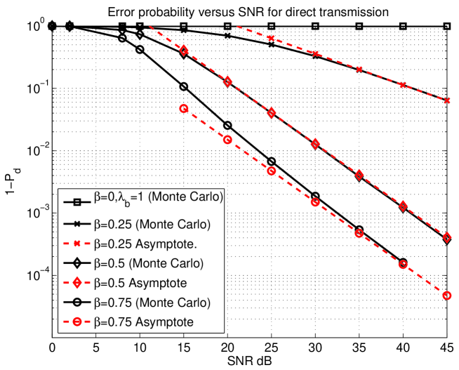
Figure 2: Outage probability $1-\mathsf{P}_{d}$ versus $\mathsf{SNR}$ for $\lambda_{b}=\mathsf{SNR}^{-\beta}$ with different $\beta$. The system parameters are $\alpha=4$, $\theta=1.5$, $r(o)=(0.5,0.5)$ and $\ell(x)=(1+\|x\|^{4})^{-1}$. The dashed lines are the asymptotes derived in (12). Observe the difference in the slopes of the error curve for $\beta<0.5$ and $\beta\geq 0.5$.

In the scaling law provided, observe that the distance of the receiver from the BS is fixed.

III-B Properties of the potential relay sets $\hat{\Phi}(x)$.

In this subsection, the properties of the node set that the BS at the origin is able to connect to are analyzed. When the BSs transmit, the interference seen by two MSs is independent. So the set of MSs to which the BS at the origin can connect to is an independent thinning of $\Phi_{o}$. Hence $\hat{\Phi}(o)$ is also a PPP and since the thinning depends on the position, the resulting process is inhomogeneous. Hence the intensity of $\hat{\Phi}(o)$ is

$$\delta(x)=\eta(x)\mathbb{E}\mathbf{1}(o\rightarrow x\mid\Phi_{b}\setminus\{o\}).$$

Following a procedure similar to the derivation of (10), the intensity is given by

$$\delta(x)=\eta(x)\exp\left(-\frac{\theta}{\mathsf{SNR}}\frac{\ell(R)}{\ell(x)}\right)\Delta(x).$$ (13)

The average number of MSs which the BS is able to connect to is

$$\mathbb{E}\sum_{x\in\Phi_{o}}\mathbf{1}(o\rightarrow x\mid\Phi_{b}\setminus\{o\}) = \int_{\mathbb{R}^{2}}\delta(x)\mathrm{d}x,$$ (14)

which follows from the Campbell-Mecke theorem [10]. The average distance over which the BS at the origin can connect is

$$L = \frac{\mathbb{E}\sum_{x\in\Phi_{o}}\|x\|\mathbf{1}(o\rightarrow x\mid\Phi_{b})}{\mathbb{E}\sum_{x\in\Phi_{o}}\mathbf{1}(o\rightarrow x\mid\Phi_{b})}$$ (15)

$$= \frac{\int_{\mathbb{R}^{2}}\|x\|\delta(x)\mathrm{d}x}{\int_{\mathbb{R}^{2}}\delta(x)\mathrm{d}x}.$$ (16)

In the second hop, a subset of the MSs which were able to receive information in the first-hop transmit. In the next sections we analyze the following two strategies to select a subset $R_{x}\subset\hat{\Phi}(x)$ to transmit in the second hop (odd time slots):

• The MS closest to the destination and that has received information in the first hop transmits in the second hop. This strategy requires nodes to know their respective locations.

• The MS with the best channel (fading and path-loss) to the destination that has received information in the first hop transmits. This strategy requires the relays to have channel state information.

IV Method 1: Nearest Relay to the Destination Transmits

In this relay selection method, the node $x\in\hat{\Phi}(a),a\in\Phi_{b}$, closest to $r(a)$ is selected to transmit in the second hop. To do this each node should know its own location, and each packet should have location information about its destination. For a fair comparison with the direct transmission scheme, we assume that the selected relay transmits with power $\mathsf{SNR}\sigma^{2}/\ell(R)$. The probability of success in this relay selection method is

$$\mathsf{P}_{r} = \mathbb{P}\left(\mathsf{h}_{x,r(o)}\ell(r)>\theta(\sigma^{2}+I)\right),$$

where $I$ is the inter cell interference at $r(o)$, and $r$ is the distance from the relay in the set $\hat{\Phi}(o)$ that is nearest to $r(o)$. More precisely

$$r=\left\{\begin{array}[]{ll}\inf_{x\in\hat{\Phi}(o)}\|x-r(o)\|,&|\hat{\Phi}(o)|>0\\ \infty,&|\hat{\Phi}(o)|=0.\end{array}\right.$$

$\hat{\Phi}(o)$ can be empty because of the following two reasons:

1. The cell has no MS to begin with. The probability of this happening is $1-\mu$.

2. The BS was not able to connect to any MS in the first time slot.

For a fair comparison with direct transmission, we condition on the cell at the origin having at least one MS to begin with, i.e., $n_{o}>0$. So

$$\mathsf{P}_{r}\mid(n_{o}>0)=\mathsf{P}_{r}\mu^{-1}.$$

Let $F_{o}(r,\mathsf{SNR},\lambda_{b})$ denote the CDF of the first contact distribution of $\hat{\Phi}(o)$ from $r(o)$. It is given by

$$F_{o}(r,\mathsf{SNR},\lambda_{b}) = 1-\exp\left(-\int_{B(r(o),r)}\delta(x)\mathrm{d}x\right).$$ (17)

Observe that $F_{o}(r,\mathsf{SNR},\lambda_{b})$ is a defective distribution, i.e., $F_{0}(\infty,\mathsf{SNR},\lambda_{b})<1$. Let

$$f_{o}(r,\mathsf{SNR},\lambda_{b})=-\frac{\partial}{\partial r}F_{o}(r,\mathsf{SNR},\lambda_{b})$$

denote the PDF of the first contact distribution. Hence

$$\mathsf{P}_{r} = \int_{0}^{\infty}\exp\left(-\frac{\theta\ell(R)}{\mathsf{SNR}\ell(r)}\right)\underbrace{\mathbb{E}\left(\exp\left(-\frac{\theta\ell(R)}{\mathsf{SNR}\sigma^{2}\ell(r)}I\right)\right)}_{T_{1}(\lambda_{b},r)}f_{o}(r,\mathsf{SNR},\lambda_{b})\mathrm{d}r.$$

where $I$ is the interference at $r(o)$ caused by transmitters in other cells. Even though $\int f_{o}(r,\mathsf{SNR},\lambda_{b})\mathrm{d}r<1$ the above average is correct since the integrand is zero at $r=\infty$ where the remaining mass of the first contact distribution lies. We now evaluate $T_{1}(\lambda_{b},r)$. Let $f_{a}(x),a\neq 0$, $x\in\mathbb{R}^{2}$, denote the PDF of the nearest neighbor of $r(a)$ in the set $\hat{\Phi}(a)$ relative to $a$, conditioned on the event $|\hat{\Phi}(a)|>0$. We then have

$$T_{1}(\lambda_{b},r)=\prod_{a\in\mathbb{Z}^{2}\setminus\{o\}}\int_{\mathbb{R}^{2}}\mathbb{E}\left[\frac{f_{a}(x)}{1+\frac{\theta}{\ell(r)}\ell(\frac{a}{\sqrt{\lambda_{b}}}+x-r(o))\mathbf{1}(|\hat{\Phi}(a)|>0)}\right]\mathrm{d}x$$

Taking the average with respect to $|\hat{\Phi}(a)|$ yields

$$\prod_{a\in\mathbb{Z}^{2}\setminus\{o\}}\int_{\mathbb{R}^{2}}\mathbb{E}\left[1-\mathbf{1}(|\hat{\Phi}(a)|>0)+\frac{f_{a}(x)\mathbf{1}(|\hat{\Phi}(a)|>0)}{1+\frac{\theta}{\ell(r)}\ell(\frac{a}{\sqrt{\lambda_{b}}}+x-r(o))}\right]\mathrm{d}x$$

$$\prod_{a\in\mathbb{Z}^{2}\setminus\{o\}}1-\int_{\mathbb{R}^{2}}\frac{f_{a}(x)(1-\exp(-\int\delta(y)\mathrm{d}y))}{1+\frac{\ell(r)}{\theta}\ell(\frac{a}{\sqrt{\lambda_{b}}}+x-r(o))^{-1}}\mathrm{d}x.$$

$f_{a}(x)$ depends on the geometry of each cell, $\delta(x)$, $r(a)$, and is easy to calculate once these quantities are known. We now calculate the asymptotics of $\mathsf{P}_{r}$ and the asymptotic gain.
Asymptotic gain: In this part we scale the BS density as $\lambda_{b}=\mathsf{SNR}^{-\beta}$. It is easy to observe that the average number of MS in each cell that are potential relays, i.e., $\int\delta(x)\mathrm{d}x$, scales as

$$\int\delta(x)\mathrm{d}x\sim\int\eta(x)\mathrm{d}x-\frac{\theta\ell(R)}{\mathsf{SNR}}\int\frac{\eta(x)}{\ell(x)}\mathrm{d}x-\frac{\theta C(\alpha)}{\mathsf{SNR}^{\alpha\beta/2}}\int\frac{\eta(x)}{\ell(x)}\mathrm{d}x.$$ (18)

It can also be verified that

$$\sup_{r}|F_{o}(r,\mathsf{SNR},\mathsf{SNR}^{-\beta})-F_{o}(r,\infty,0)|\rightarrow 0$$

as $\mathsf{SNR}\rightarrow\infty$, which implies $F_{o}(r,\mathsf{SNR},\mathsf{SNR}^{-\beta})$ converges uniformly to $F_{o}(r,\infty,0)$. Hence we can interchange the derivative and the limit in the asymptotic analysis. We have

$$f_{o}(r,\mathsf{SNR},\mathsf{SNR}^{-\beta})=\exp\left(-\int_{B(r(o),r)}\delta(x)\mathrm{d}x\right)\frac{\partial}{\partial r}\int_{B(r(o),r)}\delta(x)\mathrm{d}x.$$

From (18) and the fact that $\exp(-x)\sim 1-x$ for small $x$ it follows that,

$$f_{o}(r,\mathsf{SNR},\mathsf{SNR}^{-\beta})\sim\left\{\begin{array}[]{ll}\exp\left(-f(r)\right)\left(\frac{\partial}{\partial r}f(r)-\frac{\theta\ell(R)}{\mathsf{SNR}}g(r)\right)&\alpha\beta>2\\ \exp\left(-f(r)\right)\left(\frac{\partial}{\partial r}f(r)-\frac{\theta C(\alpha)}{\mathsf{SNR}^{\alpha\beta/2}}g(r)\right)&\alpha\beta<2\end{array}\right.$$

where

$$g(r)=\frac{\partial}{\partial r}\int_{B(r(o),r)}\frac{\eta(x)}{\ell(x)}\mathrm{d}x-\int_{B(r(o),r)}\frac{\eta(x)}{\ell(x)}\mathrm{d}x\frac{\partial}{\partial r}f(r),$$

and

$$f(r)=\int_{B(r(o),r)}\eta(x)\mathrm{d}x.$$

The following limit follows similar to the asymptotic analysis of $\mathsf{P}_{d}$

$$\lim_{\mathsf{SNR}\rightarrow\infty}\frac{1-T_{1}(\mathsf{SNR}^{-\beta},r)}{\mathsf{SNR}^{-\beta\alpha/2}}=\frac{\theta C(\alpha)\mu}{\ell(r)},$$

where $C(\alpha)$ is given by (11). By some basic algebraic manipulations the asymptotic expansion of the error probability with respect to $\mathsf{SNR}$ with $\lambda_{b}=\mathsf{SNR}^{-\beta},\beta>0$, is

$$1-\mathsf{P}_{2}\mid(n_{o}>0)\sim\left\{\begin{array}[]{ll}\frac{\theta\ell(R)}{\mathsf{SNR}\mu}\int_{0}^{\infty}\exp\left(-f(r)\right)\left\{g(r)+\ell(r)^{-1}\frac{\partial}{\partial r}f(r)\right\}\mathrm{d}r&\alpha\beta>2\\ \frac{\theta C(\alpha)}{\mathsf{SNR}^{\alpha\beta/2}\mu}\int_{0}^{\infty}\exp\left(-f(r)\right)\left\{g(r)+\mu\ell(r)^{-1}\frac{\partial}{\partial r}f(r)\right\}\mathrm{d}r&\alpha\beta<2.\end{array}\right.$$ (19)

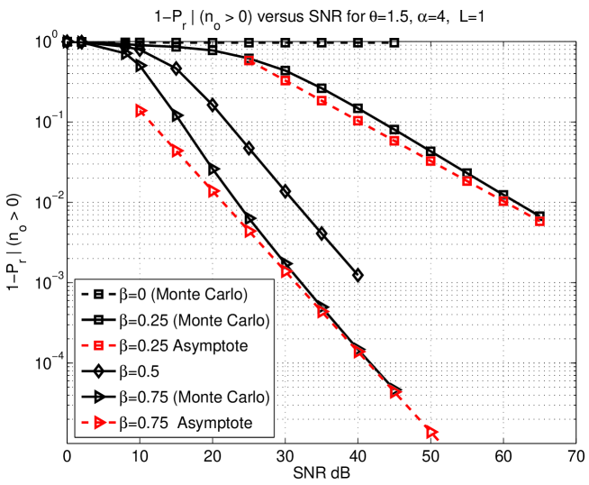
Figure 3: Outage probability $1-\mathsf{P}_{r}\mid(n_{o}>0)$ versus $\mathsf{SNR}$ for $\lambda_{b}=\mathsf{SNR}^{-\beta}$ for different $\beta$. The system parameters are $\alpha=4$, $\theta=1.5$, $r(o)=(0.5,0.5)$, $\ell(x)=(1+\|x\|^{4})^{-1}$ and $\eta(y)=5\mathbf{1}_{y}([-0.5,0.5]^{2})$. The dashed lines are the asymptotes derived in (19). The dashed lines are the asymptotes derived in (19) and are approximately equal to $10.351\mathsf{SNR}^{-0.5}$ (interference-limited) and $1.387\mathsf{SNR}^{-1}$ (noise-limited).

These asymptotes are plotted in Figure 3. From (19) the asymptotic gain is

$$\lim_{\mathsf{SNR}\rightarrow\infty}G(\mathsf{SNR},\mathsf{SNR}^{-\beta})\sim\left\{\begin{array}[]{ll}\mu\ell(R)^{-1}\left(\int_{0}^{\infty}\exp\left(-f(r)\right)\left\{g(r)+\ell(r)^{-1}\frac{\partial}{\partial r}f(r)\right\}\mathrm{d}r\right)^{-1}&\alpha\beta>2\\ \mu\ell(R)^{-1}\left(\int_{0}^{\infty}\exp\left(-f(r)\right)\left\{g(r)+\mu\ell(r)^{-1}\frac{\partial}{\partial r}f(r)\right\}\mathrm{d}r\right)^{-1}&\alpha\beta<2.\end{array}\right.$$

Remarks:

• We observe that the gain is higher in the interference-limited regime than the noise-limited regime. This is because in this relay selection method, some of the cells may not be able to transmit because they do not contain any MS, which happens with probability $1-\mu$.

• Since the gain does not scale with $\mathsf{SNR}$, the diversity of this scheme is also equal to $\min\{1,\beta\alpha/2\}$. See Figure 3 for the error plot obtained by Monte Carlo simulations and the above asymptotes obtained theoretically.

V Method 2: Relay With Best Channel to the Destination Transmits(Selection Cooperation).

In this selection procedure, the fading between a potential relay and the destination is also included in the criterion for the relay selection. The relay with the best channel to the destination is selected. This method of relay selection is called selection cooperation. In the second hop, each relay of the set $\hat{\Phi}(o)$ can send a channel estimation packet to the destination in an orthogonal fashion, and the destination can choose the relay with the best channel. Alternatively, if channel reciprocity is assumed, the relays can estimate the channel between themselves and the destination when receiving the NACK and use this information to elect the best relay in a distributed fashion.

As in the previous section we shall find the success probability conditioned on the cell at the origin being non-empty, i.e., $\mathsf{P}_{r}\mid n_{o}>0$. As indicated earlier

$$\mathsf{P}_{r}\mid(n_{o}>0)=\mu^{-1}\mathsf{P}_{r}.$$

Hence we shall first calculate the unconditional probability $\mathsf{P}_{r}$ and then multiply it with $\mu^{-1}$. The relay that is selected is mathematically described by

$$\operatorname{arg~{}max}_{x\in\hat{\Phi}(o)}\{\mathsf{h}_{xr(o)}\ell(x-r(o))\}.$$

The exact analysis of this relay selection in the presence of interference is difficult and hence our aim in this section is to obtain the scaling behaviour of $G(\mathsf{SNR},\mathsf{SNR}^{-\beta/2})$. Let $k$ denote the cardinality of the set $\hat{\Phi}(o)$. Since the connectivity in the first hop is independent across relays, $k$ is a Poisson random variable with mean

$$\mathbb{E}[k]=\int_{\mathbb{R}^{2}}\delta(x)\mathrm{d}x.$$

To make the comparison with the direct transmission easier, we assume that each node transmits with power $P=\mathsf{SNR}\sigma^{2}/\ell(R)$. The probability of error is

$$1-\mathsf{P}_{r}=\mathbb{P}\left(P\max_{x\in\hat{\Phi}(o)}\{\mathsf{h}_{xr(o)}\ell(x-r(o))\}<\theta(I+\sigma^{2})\right),$$

where $I$ is the interference at $r(o)$ caused by concurrent transmissions in other cells. Conditioning on the point set $\hat{\Phi}(o)$ we have

$$1-\mathsf{P}_{r}\mid\hat{\Phi}(o) = \mathbb{P}\left(P\max_{x\in\hat{\Phi}(o)}\{\mathsf{h}_{xr(o)}\ell(x-r(o))\}<\theta(I+\sigma^{2})\mid\hat{\Phi}(o)\right)$$

$$= \mathbb{E}\left[\prod_{x\in\hat{\Phi}(o)}1-\exp\left(-\frac{\theta(\sigma^{2}+I)}{P\ell(x-r(o))}\right)\mid\hat{\Phi}(o)\right].$$

Since $\hat{\Phi}(o)$ is a PPP with intensity function $\delta(x)$, conditioning on there being $k$ points in the set, each node in the set is independently distributed with density $\kappa(x)=\frac{\delta(x)}{\int_{\mathbb{R}^{2}}\delta(y)\mathrm{d}y}$. Removing the conditioning on the locations of $\hat{\Phi}(o)$, we obtain

$$1-\mathsf{P}_{r}\mid(|\hat{\Phi}(o)|=k)=\mathbb{E}\left[1-\int_{\mathbb{R}^{2}}\exp\left(-\frac{\theta(\sigma^{2}+I)}{P\ell(x-r(o))}\right)\kappa(x)\mathrm{d}x\right]^{k}$$ (20)

Using binomial expansion,

$$1-\mathsf{P}_{r}\mid(|\hat{\Phi}(o)|=k)=\underbrace{\mathbb{E}\left[\sum_{m=0}^{k}(-1)^{m}{k\choose m}\mathbb{E}\left[\int_{\mathbb{R}^{2}}\exp\left(-\frac{\theta(\sigma^{2}+I)}{P\ell(x-r(o))}\right)\kappa(x)\mathrm{d}x\right]^{m}\right]}_{a_{k}}.$$

Hence $1-\mathsf{P}_{r}\mid(|\hat{\Phi}(o)|=k)$ is equal to

$$\sum_{m=0}^{k}(-1)^{m}{k\choose m}\int_{\mathbb{R}^{2m}}\nu(x_{1},\ldots,x_{m})\exp\left(-\frac{\theta\sigma^{2}\sum_{b=1}^{m}\ell(x_{b}-r(o))^{-1}}{P}\right)\prod_{b=1}^{m}\kappa(x_{b})dx_{1}\ldots\mathrm{d}x_{m},$$

where

$$\nu(x_{1},\ldots,x_{m}) = \mathbb{E}\left[\prod_{b=1}^{m}\exp\left(-\frac{I\theta}{\ell(x_{b}-r(o))}\right)\right]$$

$$= \mathbb{E}\left[\exp\left(-I\theta\varrho(x_{1}^{m})\right)\right]$$

$$= \mathbb{E}\left[\exp\left(-\theta\varrho(x_{1}^{m})\sum_{a\in\mathbb{Z}^{2}}\mathsf{h}_{y(a)r(o)}\ell(y(a)-r(o))\mathbf{1}(|\hat{\Phi}(a)|>0)\right)\right]$$

where $y(a)$ denotes the location of the selected relay in the cell at $a$ and $\varrho(x_{1}^{m})=\sum_{b=1}^{m}\ell(x_{b}-r(o))^{-1}$. Let $g_{a}(x)$ denote the PDF of $a-x$ where

$$x=\operatorname{arg~{}max}_{x\in\hat{\Phi}(a)}\{\mathsf{h}_{xr(a)}\ell(x-r(a))\}.$$

$g_{a}(x)$ is difficult to calculate and is the reason of resorting to asymptotics. Since $\mathsf{h}_{y(a)r(o)}$ is exponential it follows that

$$\nu(x_{1},\ldots,x_{m})=\prod_{a\in\mathbb{Z}^{2}}1-\int_{\mathbb{R}^{2}}\frac{g_{a}(y)(1-\exp(-\int\delta(x)\mathrm{d}x)}{1+\theta^{-1}\varrho(x_{1}^{m})^{-1}\ell(y+\frac{a}{\sqrt{\lambda_{b}}}-r(o))^{-1}}\mathrm{d}y.$$

Hence the unconditional probability of error is

$$\mathsf{P}_{r}=\mu^{-1}\left[1-\exp\left(-\int_{\mathbb{R}^{2}}\delta(x)\mathrm{d}x\right)\sum_{k=0}^{\infty}a_{k}\frac{(\int\delta(x)\mathrm{d}x)^{k}}{k!}.\right]$$

Asymptotic gain: The above expansion is too unwieldy to yield any asymptotics. We shall use (20) to obtain the gain in the high-$\mathsf{SNR}$ and low-interference regime. Removing the conditioning in (20) we have

$$1-\mathsf{P}_{r}=\mathbb{E}\exp\left[-\int_{\mathbb{R}^{2}}\exp\left(-\frac{\theta(\sigma^{2}+I)}{P\ell(x-r(o))}\right)\delta(x)\mathrm{d}x\right].$$

The above result follows from the generating function of a Poisson random variable. Hence the required conditional probability is

$$\mathsf{P}_{r}\mid(n_{o}>0) = \mu^{-1}\left(1-\mathbb{E}\exp\left[-\int_{\mathbb{R}^{2}}\exp\left(-\frac{\theta(\sigma^{2}+I)}{P\ell(x-r(o))}\right)\delta(x)\mathrm{d}x\right]\right).$$

An upper bound follows from Jensen’s inequality:

$$\mathsf{P}_{r}\mid(n_{o}>0)\leq\mu^{-1}\left(1-\exp\left[-\int_{\mathbb{R}^{2}}\mathbb{E}\exp\left(-\frac{\theta(\sigma^{2}+I)}{P\ell(x-r(o))}\right)\delta(x)\mathrm{d}x\right]\right).$$

Similarly a lower bound can be obtained by using the inequality $\exp(-x)\geq 1-x$ for the inner $\exp$,

$$\mathsf{P}_{r}\mid(n_{o}>0) \geq \mu^{-1}\left(1-\exp\left(-\int_{\mathbb{R}^{2}}\delta(x)\mathrm{d}x\right)\mathbb{E}\exp\left(\int_{\mathbb{R}^{2}}\frac{\theta(\sigma^{2}+I)}{P\ell(x-r(o))}\delta(x)\mathrm{d}x\right)\right).$$

To evaluate the upper and lower bounds we observe that we will have to find $\mathbb{E}[\exp(-sI)]$. By a procedure similar to the derivation of $\nu(x_{1},\ldots,x_{m})$:

$$\mathbb{E}[\exp(-sI)]=\prod_{a\in\mathbb{Z}^{2}}1-\int_{\mathbb{R}^{2}}\frac{g_{a}(y)(1-\exp(-\int\delta(x)\mathrm{d}x)}{1+s^{-1}\ell(y+\frac{a}{\sqrt{\lambda_{b}}}-r(o))^{-1}}\mathrm{d}y.$$

Recall that $\delta(x)$ is equal to

$$\eta(x)\exp\left(-\frac{\theta}{\mathsf{SNR}}\frac{\ell(R)}{\ell(x)}\right)\prod_{y\in\mathbb{Z}^{2}\setminus\{o\}}\frac{1}{1+\frac{\theta}{\ell(x)}\ell(y/\sqrt{\lambda_{b}}-x)}.$$

We now find the asymptotic lower and upper bound when $\lambda_{b}=\mathsf{SNR}^{-\beta}$ for large $\mathsf{SNR}$. We first observe that

$$\delta(x)\sim\eta(x)\left(1-\frac{\theta\ell(R)}{\ell(x)}\mathsf{SNR}^{-1}-\frac{\theta}{\ell(x)}C(\alpha)\mathsf{SNR}^{-\alpha\beta/2}\right).$$

It is also easy to obtain that

$$\mathbb{E}[\exp(-sI)]\sim 1-\mu sC(\alpha).$$

After basic algebraic manipulation, it is established that both the upper and the lower bounds exhibit the same scaling which is

$$\mathsf{P}_{r}\mid(n_{o}>0)\sim\left\{\begin{array}[]{ll}1-\mathsf{SNR}^{-1}\left(\frac{1-\mu}{\mu}\right)\theta\ell(R)\int_{\mathbb{R}^{2}}\left[\frac{1}{\ell(x-r(o))}+\frac{1}{\ell(x)}\right]\eta(x)\mathrm{d}x&\alpha\beta>2\\ 1-\mathsf{SNR}^{-\alpha\beta/2}\left(\frac{1-\mu}{\mu}\right)\theta C(\alpha)\int_{\mathbb{R}^{2}}\left[\frac{\mu}{\ell(x-r(o))}+\frac{1}{\ell(x)}\right]\eta(x)\mathrm{d}x&\alpha\beta<2.\end{array}\right.$$ (21)

Hence the gain is

$$\lim_{\mathsf{SNR}\rightarrow\infty}G(\mathsf{SNR},\mathsf{SNR}^{-\beta})=\left\{\begin{array}[]{ll}\frac{\mu}{1-\mu}\ell(R)^{-1}\left[\int_{\mathbb{R}^{2}}\left[\frac{1}{\ell(x-r(o))}+\frac{1}{\ell(x)}\right]\eta(x)\mathrm{d}x\right]^{-1}&\alpha\beta>2\\ \frac{\mu}{1-\mu}\ell(R)^{-1}\left[\int_{\mathbb{R}^{2}}\left[\frac{\mu}{\ell(x-r(o))}+\frac{1}{\ell(x)}\right]\eta(x)\mathrm{d}x\right]^{-1}&\alpha\beta<2\end{array}\right.$$ (22)

Hence the diversity of this scheme is

$$\mathrm{d}_{2}(\mathsf{SNR}^{-\beta})=\min\left\{1,\frac{\alpha\beta}{2}\right\}.$$

In the above analysis we assumed that the cell is non-empty and hence obtained a maximum diversity of $1$.

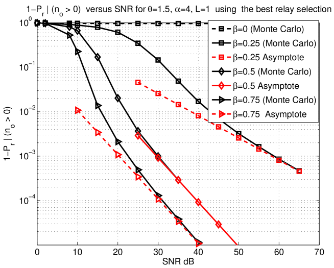
Figure 4: Outage probability $1-\mathsf{P}_{r}\mid(n_{o}>0)$ versus $\mathsf{SNR}$ for $\lambda_{b}=\mathsf{SNR}^{-\beta}$ and various $\beta$. The system parameters are $\alpha=4$, $\theta=1.5$, $z=(0.5,0.5)$, $\ell(x)=(1+\|x\|^{4})^{-1}$ and $\eta(y)=5\mathbf{1}_{y}([-0.5,0.5]^{2})$. The dashed lines are the asymptotes derived in (21) and are approximately equal to $0.812\mathsf{SNR}^{-0.5}$(interference limited) and $0.108\mathsf{SNR}^{-1}$ (noise limited).

VI Simulation Results and Observations

In this section the gain of the proposed methods over direct transmission is obtained by Monte-Carlo simulations. For the purpose of simulation we truncate the BS lattice to $\lambda_{b}^{-1/2}\{-2,-1,0,1,2\}^{2}$, and $\theta=1.5$ is used as the decoding threshold. The cells are modeled as squares and the destination of each BS is located at a random vertex of the square. The spatial density used is

$$\eta(y)=\lambda_{m}\mathbf{1}_{y}([-L/2,L/2]^{2}).$$

If not specified we use $\lambda_{m}=5$ and $L=1$.

()<++> In Figures 3 and 4 the error probability of the schemes employing nearest relay to the destination and the best relay are plotted. We observe that the asymptotes obtained from theory match perfectly with the simulation results. As predicted by theory, the diversity obtained is $1$ when $\alpha\beta>2$ and is equal to $\alpha\beta/2$ otherwise. From Figure 5 and 6, it can be seen that the gain reaches a constant when $\mathsf{SNR}\rightarrow\infty$.

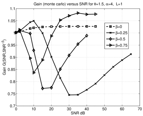
Figure 5: $G(\mathsf{SNR},\mathsf{SNR}^{-\beta})$ versus $\mathsf{SNR}$ for various $\beta$. Relay closest to the destination is selected.

Figure 6: $G(\mathsf{SNR},\mathsf{SNR}^{-\beta})$ versus $\mathsf{SNR}$ for various $\beta$. Relay with the best channel to the destination is selected.

We observe that the best-relay selection scheme performs the best as expected.

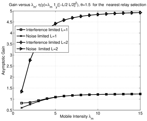
Figure 7: Asymptotic gain versus $\lambda_{m}$ where $\lambda_{m}$ is the intensity in $\eta(y)=\lambda_{m}\mathbf{1}_{y}([-L/2,L/2]^{2})$, $\ell(x)=\|x\|^{-\alpha}$, $\theta=1.5$ and $z=(-L/2,L/2)$.

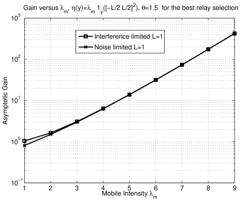
Figure 8: Asymptotic gain versus $\lambda_{m}$ where $\lambda_{m}$ is the intensity in $\eta(y)=\lambda_{m}\mathbf{1}_{y}([-L/2,L/2]^{2})$, $\ell(x)=\|x\|^{-\alpha}$, $\theta=1.5$ and $z=(-L/2,L/2)$.

In Figure 8, we observe that the asymptotic gain increases exponentially with $\lambda_{m}$ because of the $(1-\mu)/\mu$ factor in the expression for the asymptotic gain. Setting $\lambda_{b}=\mathsf{SNR}^{-\beta}$ reduces the spatial reuse factor as the $\mathsf{SNR}$ increases. The effective throughput density of the network is equal to $\mathsf{P}_{2}\log(1+\theta)\mathsf{SNR}^{-\beta}$ and the maximum of this throughput density is the transmission capacity [13]. In Figure 9, we plot $(\mathsf{P}_{2}\mid n_{o}>0)\log(1+\theta)\mathsf{SNR}^{-\beta}$ versus $\mathsf{SNR}$ for various $\beta$. We observe that for each $\mathsf{SNR}$ there is a $\beta$ that maximizes the throughput density, and that as $\mathsf{SNR}\rightarrow\infty$, the maximizing $\beta$ tends to $0$, which is intuitive. The figure indicates that a throughput density of $\approx 0.1\text{bps}/\text{m}^{2}$ is achieved at low $\mathsf{SNR}$, and that it increases with $\mathsf{SNR}$.

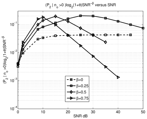
Figure 9: $(\mathsf{P}_{2}\mid n_{o}>0)\log_{2}(1+\theta)\mathsf{SNR}^{-\beta}$ versus $\mathsf{SNR}$ for various $\beta$. The best relay selection scheme is used.

VII Conclusions

In this paper we have analyzed the outage in a two-hop cellular system under consideration of all the node location statistics. Outage results were provided for two relay selection schemes, namely nearest-relay selection and best-relay selection. We observed that the diversity obtained is $\min\{1,\alpha\beta/2\}$ where $\alpha$ is the path-loss exponent, when the density of the base stations scale as $\lambda_{b}=\mathsf{SNR}^{-\beta}$ (alternatively $\mathsf{SIR}=\Theta(\mathsf{SNR}^{\alpha\beta/2})$). From this result we can infer that the system is noise-limited (even for high $\mathsf{SNR}$) when $\alpha\beta>2$ and interference-limited otherwise. The asymptotic outage gain of the two-hop system over direct transmission takes only two values as a function of $\beta$ depending on the relay selection scheme. The gain in selecting a relay with the best channel over a direct transmission increases exponentially with the density of the available relays. The gain also increases with increasing source-destination distance. From simulations we conclude that the gain in selecting the best relay outweighs the overhead in estimating the fading coefficients between the relays and the destination as compared to the near-relay selection method. The techniques introduced in this paper can be extended for the spatial analysis of other relay selection schemes.

References

- [1] G. Neonakis Aggelou and R. Tafazolli, “On the relaying capability of next-generation GSM cellular networks,” Personal Communications, IEEE, vol. 8, pp. 40–47, Feb 2001.
- [2] H. yu Wei and R. Gitlin, “Two-hop-relay architecture for next-generation WWAN/WLAN integration,” Wireless Communications, IEEE, vol. 11, pp. 24–30, Apr 2004.
- [3] V. Sreng, H. Yanikomeroglu, and D. Falconer, “Coverage enhancement through two-hop relaying in cellular radio systems,” in 2002 IEEE Wireless Communications and Networking Conference, 2002. WCNC2002, vol. 2, 2002.
- [4] Z. Jingmei, S. Chunju, W. Ying, and Z. Ping, “Performance of a two-hop cellular system with different power allocation schemes,” in 2004 IEEE 60th Vehicular Technology Conference, 2004. VTC2004-Fall, vol. 6, 2004.
- [5] J. Laneman and G. Wornell, “Distributed space-time coded protocols for exploiting cooperative diversity in wireless networks,” in IEEE Global Telecommunications Conference, 2002. GLOBECOM’02, vol. 1, 2002.
- [6] J. Laneman, D. Tse, and G. Wornell, “Cooperative diversity in wireless networks: Efficient protocols and outage behavior,” IEEE Transactions on Information Theory, vol. 50, no. 12, pp. 3062–3080, 2004.
- [7] A. Bletsas, A. Khisti, D. Reed, and A. Lippman, “A simple cooperative diversity method based on network path selection,” IEEE Journal on Selected Areas in Communications, vol. 24, no. 3, pp. 659–672, 2006.
- [8] E. Beres and R. Adve, “On selection cooperation in distributed networks,” in Information Sciences and Systems, 2006 40th Annual Conference on, pp. 1056–1061, 2006.
- [9] D. Michalopoulos and G. Karagiannidis, “Performance analysis of single relay selection in Rayleigh fading,” IEEE Transactions on Wireless Communications, vol. 7, pp. 3718–3724, October 2008.
- [10] D. Stoyan, W. S. Kendall, and J. Mecke, Stochastic Geometry and its Applications. Wiley series in probability and mathematical statistics, New York: Wiley, second ed., 1995.
- [11] D. J. Daley and D. Vere-Jones, An Introduction to the Theory of Point Processes. New York: Springer, second ed., 1998.
- [12] A. Edery, “Multidimensional cut-off technique, odd-dimensional Epstein zeta functions, and Casimir energy of massless scalar fields,” J. Phys. A: Math. Gen. 39, pp. 685–712, 2006.
- [13] S. Weber, X. Yang, J. Andrews, and G. de Veciana, “Transmission capacity of wireless ad hoc networks with outage constraints,” Information Theory, IEEE Transactions on, vol. 51, no. 12, pp. 4091–4102, 2005.