The viscous friction of a mesh-like super-hydrophobic surface

The friction of a mesh-like super-hydrophobic surface

Abstract

When a liquid droplet is located above a super-hydrophobic surface, it only barely touches the solid portion of the surface, and therefore slides very easily on it. More generally, super-hydrophobic surfaces have been shown to lead to significant reduction of viscous friction in the laminar regime, so it is of interest to quantify their effective slipping properties as a function of their geometric characteristics. Most previous studies have considered flows bounded by arrays of either long grooves, or isolated solid pillars on an otherwise flat solid substrate, and for which therefore the surrounding air constitutes the continuous phase. Here we consider instead the case where the super-hydrophobic surface is made of isolated holes in an otherwise continuous no-slip surface, and specifically focus on the mesh-like geometry recently achieved experimentally. We present an analytical method to calculate the friction of such a surface in the case where the mesh is thin. The results for the effective slip length of the surface are computed, compared to simple estimates, and a practical fit is proposed displaying a logarithmic dependance on the area fraction of the solid surface.

I Introduction

Among the fascinating flow phenomena occurring on small scales stone_review ; squiresquake , super-hydrophobicity offers a unique bridge between microscopic features and macroscopic behavior feng02 ; quere05 ; sun05 ; quere08 . Super-hydrophobic surfaces are non-wetting surfaces which possess sufficiently-large geometrical roughness that a liquid droplet deposited on the surface would not fill the grooves of the surface roughness, but instead remain in a a fakir-like state where the droplet only touches the surface at the edge of the roughness (Fig. 1a). As a result, super-hydrophobic surfaces possess very high effective contact angles, and display remarkable macro-scale wetting properties feng02 ; quere05 ; sun05 ; quere08 .

One particularly interesting characteristic of super-hydrophobic surfaces is their low viscous friction. Since fluid in contact with the surface only barely touches it, but is instead mostly in contact with the surrounding air, small droplets can roll very easily, a phenomenon known as the lotus-leaf effect. In general, super-hydrophobic surfaces are expected to provide opportunities for significant drag reduction in the laminar regime, as has been confirmed by experiments cited below. The effective viscous friction of a solid surface is usually quantified by a so-called slip length, denoted here by $\lambda$, which is the distance below the solid surface where the no-slip boundary would be satisfied if the flow field was linearly extrapolated, and the no-slip boundary condition corresponds to $\lambda=0$ neto05 ; laugareview ; bocquet07 .

At low Reynolds number, the only characteristics affecting the friction of super-hydrophobic surfaces arise from their geometry, specifically (a) the distribution of liquid/solid and liquid/air contact at the edge of the roughness elements of the surface, and (b) the shape of the liquid/air free surface. For one-dimensional surfaces, i.e. surfaces which have one homogeneous direction (Fig. 1b), significant drag reduction can be obtained when the homogeneous direction is parallel or perpendicular to the direction of flow, as demonstrated experimentally ou04 ; ou05 ; gogte05 ; choi06 ; truesdell06 ; maynes07 ; lee08 and theoretically philip72 ; philip72_2 ; lauga03 ; cottin-bizonne04 ; davies06 ; maynes07 ; ybert07 ; ng09 .

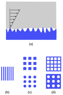
Figure 1: (color online) Typical topology of super-hydrophobic surfaces: (a) Side view of a random super-hydrophobic surface, illustrating the contact of the liquid (gray) at the edge of the surface roughness (blue); (b) Top view of a one-dimensional surface; (c) Top view of regular two-dimensional surfaces where the air (white) is the continuous phase; (d) Top view of regular two-dimensional surfaces where the solid (blue) is the continuous phase. The case illustrated on Fig. 1d (top) is the focus of the current paper.

For two-dimensional surfaces, an additional free parameter is the topology of the air/solid partition on the planar surface, and two general types can be distinguished. In the first type, the air is the continuous phase, and the liquid is in contact with the solid only at isolated, unconnected, locations (Fig. 1c). This is the most commonly-studied type of super-hydrophobic surface, and arises for surface roughness in the shape of bumps or posts on an otherwise flat solid surface ou04 ; ou05 ; gogte05 ; choi06_PRL ; joseph06 ; ybert07 ; lee08 ; ng09_2 . The second type of surface, less studied, is one where the solid is the continuous phase, and the liquid/air contact occurs on isolated domains (Fig. 1d). These surfaces can be obtained by making holes in an otherwise flat material ng09_2 , and have been used to study the influence of the geometry of the liquid/air free interface on the viscous friction of the surface steinberger07 ; hyvaluoma08 ; legendre08_2 ; davis09 .

A super-hydrophobic surface with a continuous solid phase can also be obtained by using an intertwined solid mesh. Recently this method has been exploited experimentally, using coated steel feng04 ; sun05 , and coated copper wang07 , as reproduced in Fig. 2a and b. The resulting surface is also the relevant geometrical configuration for flow past textile and fabric material. In this paper, we present an analytical method to calculate the friction of such a mesh-like (or grid-like) surface in the case where the mesh is thin in the plane (mesh aspect ratio $\epsilon\ll 1$). The analysis, based on a distribution of flow singularities, leads to an infinite system of linear equations for the approximate Fourier coefficients of the flow around the mesh, and gives results with relative error of order $\epsilon\ln(1/\epsilon)$. The results for the effective slip length of the surface are computed, compared to simple estimates, and used to propose a practical fit displaying the expected logarithmic dependance on the solid area fraction philip72 ; philip72_2 ; lauga03 ; ybert07 .

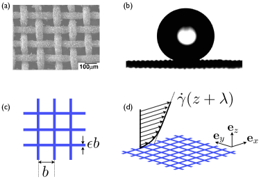
Figure 2: (color online) Mesh-like super-hydrophobic surface. (a): Coated copper mesh at the micron scale wang07 ; (b): The mesh from Figs. 2a is super-hydrophobic (water droplet, volume about 4 $\mu$l) wang07 ; (c): For our calculation we consider a planar square mesh of periodicity $b$ and width $\epsilon b$; (d): A shear flow is set up in one of the principal directions of the mesh, with shear rate $\dot{\gamma}$; the far-field flow is given by ${\bf v}=\dot{\gamma}(z+\lambda){\bf e}_{x}$, where $\lambda$ is the effective slip length of the mesh. Figs. 2a and 2b reprinted from S. Wang, Y. Song and L. Jiang (2007) “Microscale and nanoscale hierarchical structured mesh films with super-hydrophobic and superoleophilic properties induced by long-chain fatty acids”, Nanotechnology, 18, 015103, courtesy of Shutao Wang and with permission from IOP Publishing.

II Shear flow past a rectangular grid

II.1 Calculation background

Our paper follows classical work on the broadside motion of rigid bodies at low Reynolds number in the asymptotic limit for narrow cross-sections happel ; kimbook . Here, we build on the method of Leppington and Levine who studied axisymmetric potential problems involving an annular disk by using a distribution of singularities, and obtained an efficient method in the limit where the radii difference of the disk approaches zero leppington72 . Roger and Hussey studied the flat annular ring problem both experimentally and theoretically using a beads-on-a-shell model to represent a distribution of point forces roger82 . Subsequently, Stewartson showed that viscous fluid exhibits a marked reluctance to flow through a thin torus and the flux function has an essential singularity in the limit in which the hollow boundary approaches a circle and disappears stewartson83 . This ‘blockage’ feature was further demonstrated by Davis and James in considering flow through a array of narrow annular disks placed in planes normal to the flow in order to model a fibrous medium davis96 . Their analysis was made tractable by retaining only the inverse square root term in the force density function. A similar asymptotic estimate was used by Davis in modeling the broadside oscillations of a thin grid of the type discussed below davis93 . Since edgewise motions induce the same edge singularity in the force density, we follow in this paper a similar analytical treatment.

II.2 Model problem

We consider a thin stationary planar square mesh in the $(x,y)$ plane subject to a shear flow, with shear rate $\dot{\gamma}$, along the $x$ direction, which is one of the principal directions of the mesh, as illustrated in Figs. 2c and d. The mesh has periodicity $b$ and a small width $\epsilon b$. We denote by ${\bf e}_{x}$ and ${\bf e}_{y}$ the unit vectors parallel to the mesh axes, and ${\bf e}_{z}$ is the third Cartesian vector. We further assume that the shape of the interface between the liquid and the air located underneath the mesh is planar, with no protrusion of the mesh inside the fluid. Since the mesh is a super-hydrophobic surface and presents to the flow a combination of no-slip domains (the mesh) and perfectly-slipping domains (the free surfaces), the effective flow past the surface can be described as a slipping flow, and is given in the far field by ${\bf v}=\dot{\gamma}(z+\lambda){\bf e}_{x}$, where $\lambda$ is the effective surface slip length ($\lambda>0$). The goal of the calculation below is to present an accurate analytic calculation for $\lambda$ in the limit where $\epsilon\ll 1$.

In order to perform the calculation, we move in the frame translating at the steady velocity $U{\bf e}_{x}$, with $U=\dot{\gamma}\lambda$. In that case, the problem is equivalent to the uniform translation of an thin mesh in its own plane at velocity $-U{\bf e}_{x}$, and the goal is to derive the value of the shear rate $\dot{\gamma}$ in the far-field, $|z|\gg b$. The slip length will then be given by $\lambda=U/\dot{\gamma}$. Edge effects are ignored by assuming an infinite mesh as then periodic point force singularities can be used to describe the fluid flow field. The rectangular grid naturally introduces Fourier series with respect to Cartesian coordinates, and the analysis establishes a set of integral equations with the same logarithmic dependence on the geometrical parameters of the grid as in the flows described in the references discussed in §II.1.

The Reynolds number of the viscous incompressible flow is assumed to be sufficiently small for the velocity field ${\bf v}$ to satisfy the creeping flow (Stokes) equations happel ; kimbook

$$\mu\nabla^{2}{\bf v}=\nabla p,\qquad\nabla\cdot{\bf v}=0,$$ (1)

where $\mu$ is the coefficient of viscosity and $p$ is the dynamic pressure. The prescribed grid velocity is given by

$${\bf v}=-U{\bf e}_{x}\hbox{ at }z=0,\qquad(x,y)\in G.$$ (2)

In a typical grid element $0\leq x,y\leq b$, $G$ is complementary to the square hole bounded by the lines $x$ or $y=\frac{1}{2}\epsilon b$ or $(1-\frac{1}{2}\epsilon)b$ (shown in black in Fig. 3a).

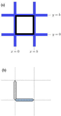
Figure 3: (color online) A typical grid element (see text for details).

II.3 Solution using a superposition of singularities

Following the calculation for broadside oscillations of the grid in Ref. davis93 , the fluid motion can be represented as due to a distribution of tangentially directed Stokeslets over the flat mesh $G$ and the density functions must be both periodic in two dimensions and symmetric with respect to the sides of each square. The field due to a two-dimensional square array, period $b$, of point forces of strength $4\pi\mu Ub$ directed parallel to the mesh’s motion, is governed by

$$\nabla\cdot{\bf v}_{A}=0$$ (3)

and

$$\mu\nabla^{2}{\bf v}_{A}-\nabla p_{A} = 4\pi\mu Ub{\bf e}_{x}\delta(z)\sum_{n_{1}=-\infty}^{\infty}\sum_{n_{2}=-\infty}^{\infty}\delta(x-n_{1}b)\delta(y-n_{2}b)$$ (4)

$$= \frac{4\pi\mu U}{b}{\bf e}_{x}\delta(z)\sum_{m_{1}=-\infty}^{\infty}\sum_{m_{2}=-\infty}^{\infty}\exp\left[\frac{2\pi i}{b}(m_{1}x+m_{2}y)\right].$$

With ${\bf m}=m_{1}{\bf e}_{x}+m_{2}{\bf e}_{y}$, the ${\bf m}={\bf 0}$ term in Eqs. (3) and (4) yields

$$\mu\nabla^{2}{\bf v}_{0}-\nabla p_{0}=\frac{4\pi\mu U}{b}{\bf e}_{x}\delta(z),\qquad\nabla\cdot{\bf v}_{0}=0,$$ (5)

whose solution,

$${\bf v}_{0}=\frac{2\pi U|z|}{b}{\bf e}_{x},\qquad p_{0}=0,$$ (6)

exhibits the anticipated shear at infinity. Note that the suppression of the immaterial arbitrary multiple of $U{\bf e}_{x}$ in ${\bf v}_{0}$ ensures uniqueness below. The solution of

$$\mu\nabla^{2}{\bf v}-\nabla p=\frac{2\mu U}{b}{\bf e}_{x}\int_{-\infty}^{\infty}e^{ikz}dk\sum_{{\bf m}}{}^{\prime}\exp\left[\frac{2\pi i}{b}{\bf m}\cdot{\bf r}\right],\qquad\nabla\cdot{\bf v}=0,$$ (7)

with a prime denoting that the ${\bf m}={\bf 0}$ term is omitted, is readily found by Fourier transform techniques (see Ref. hasimoto59 ). Thus the flow governed by Eqs. (3) and (4) is compactly expressed as

$${\bf v}_{A}=U\left[\left(\frac{2\pi|z|}{b}-S_{1}\right){\bf e}_{x}+\nabla\frac{\partial S_{2}}{\partial x}\right],\qquad p_{A}=\mu U\frac{\partial S_{1}}{\partial x},$$ (8)

where

$$S_{1}=\sum_{{\bf m}}{}^{\prime}\frac{1}{|{\bf m}|}\exp\left[\frac{2\pi}{b}(i{\bf m}\cdot{\bf r}-|{\bf m}||z|)\right]=\nabla^{2}S_{2},$$ (9)

with

$$S_{2} = -\frac{2}{b}\int_{-\infty}^{\infty}e^{ikz}dk\sum_{{\bf m}}{}^{\prime}\exp\left[\frac{2\pi i}{b}{\bf m}\cdot{\bf r}\right]\left[\left(\frac{2\pi i}{b}{\bf m}\right)^{2}+k^{2}\right]^{-2}$$ (10)

$$= -\frac{b^{2}}{8\pi^{2}}\sum_{{\bf m}}{}^{\prime}\frac{1}{|{\bf m}|^{2}}\left(\frac{1}{|{\bf m}|}+\frac{2\pi}{b}|z|\right)\exp\left[\frac{2\pi}{b}(i{\bf m}\cdot{\bf r}-|{\bf m}||z|)\right]\cdot$$

Only the velocities at the mesh and at infinity are needed for the subsequent analysis. The solution Eq. (8) shows that

$${\bf v}_{A}\sim\frac{2\pi U|z|}{b}{\bf e}_{x}{={\bf v}_{0}}\hbox{ as }|z|\to\infty,$$ (11)

since all terms in Eq. (9) exhibit exponential decay, and

$$[{\bf v}_{A}]_{z=0}=U{\bf e}_{x}\left(-S_{1}+\frac{\partial^{2}S_{2}}{\partial x^{2}}\right)_{z=0}=-U{\bf e}_{x}\sum_{{\bf m}}{}^{\prime}\frac{1}{|{\bf m}|}\exp\left[\frac{2\pi i}{b}{\bf m}\cdot{\bf r}\right]C_{{\bf m}},$$ (12)

where, after substitution of Eqs. (9) and (10), we have

$$C_{{\bf m}}=1-\frac{m_{1}^{2}}{2|{\bf m}|^{2}}\cdot$$ (13)

In particular, we see that

$$C_{(m_{1},0)}&=\frac{1}{2},\qquad C_{{\bf m}}\to\frac{1}{2}\hbox{ as }m_{1}\to\infty,\\ C_{(0,m_{2})}=1,\qquad C_{{\bf m}}\to 1\hbox{ as }m_{2}\to\infty.$$ (14)

The shaded region in Fig. 3b suffices for the distribution of periodic point forces and the enforcement of the prescribed mesh velocity (Eq. 2). The hexagon in Fig. 3b lying along the $x$-axis is given by $|y|\leq\frac{1}{2}\epsilon b,|y|\leq x\leq b-|y|$, or $-1\leq w,s\leq 1$ in terms of new variables $(w,s)$ defined by

$$w=\frac{\frac{1}{2}b-x}{\frac{1}{2}b-y},\qquad y=\frac{1}{2}\epsilon bs,\qquad x=\frac{1}{2}b[1-(1-\epsilon s)w].$$ (15)

Here $w$ may be identified as the tangent of an angle subtended at the center of the square. The hexagon in Fig. 3b lying along the $y$-axis is given similarly by interchanging $x$ and $y$ in Eq. (15). The flow generated by the translating mesh can be written as

$${\bf v} = \frac{1}{4}\int_{-1}^{1}\int_{-1}^{1}\left\{f_{x}(w,s){\bf v}_{A}\left[x-\frac{1}{2}b(1-w+\epsilon sw),y-\frac{1}{2}\epsilon bs,z\right]\right.$$ (16)

$$\left.+f_{y}(w,s){\bf v}_{A}\left[x-\frac{1}{2}\epsilon bs,y-\frac{1}{2}b(1-w+\epsilon sw),z\right]\right\}\,{\rm d}w{\rm d}s,$$

where $f_{x}$ and $f_{y}$ are dimensionless force densities. The prescribed mesh velocity is then obtained by enforcing Eq. (2) at each point of the two hexagons. Thus Eq. (16) gives

$$-U{\bf e}_{x}&=\frac{1}{4}\int_{-1}^{1}\int_{-1}^{1}\left\{f_{x}(w,s){\bf v}_{A}\left[\frac{1}{2}b(w-W+\epsilon SW-\epsilon sw),\frac{1}{2}\epsilon b(S-s),0\right]\right.\\ \left.+f_{y}(w,s){\bf v}_{A}\left[\frac{1}{2}b(1-W+\epsilon SW-\epsilon s),\frac{1}{2}b(\epsilon S-1+w-\epsilon sw),0\right]\right\}\,{\rm d}w{\rm d}s,\quad\\ -U{\bf e}_{x}=\frac{1}{4}\int_{-1}^{1}\int_{-1}^{1}\left\{f_{x}(w,s){\bf v}_{A}\left[\frac{1}{2}b(\epsilon S-1+w-\epsilon sw),\frac{1}{2}b(1-W+\epsilon SW-\epsilon s),0\right]\right.\\ \left.+f_{y}(w,s){\bf v}_{A}\left[\frac{1}{2}\epsilon b(S-s),\frac{1}{2}b(w-W+\epsilon SW-\epsilon sw),0\right]\right\}\,{\rm d}w{\rm d}s$$ (17)

for all $-1\leq W,S\leq 1$. We further note that the summation in Eq. (12) takes the simpler form

$$\sum_{{\bf m}}{}^{\prime}\frac{1}{|{\bf m}|}\exp\left[\frac{2\pi i}{b}{\bf m}\cdot{\bf r}\right]C_{{\bf m}}=\sum_{m_{1}=1}^{\infty}\frac{1}{m_{1}}\cos\frac{2\pi}{b}m_{1}x+2\sum_{m_{2}=1}^{\infty}\frac{1}{m_{2}}\cos\frac{2\pi}{b}m_{2}y$$

$$+4\sum_{m_{1}=1}^{\infty}\sum_{m_{2}=1}^{\infty}\frac{1}{\sqrt{m_{1}^{2}+m_{2}^{2}}}\left[1-\frac{m_{1}^{2}}{2(m_{1}^{2}+m_{2}^{2})}\right]\cos\frac{2\pi}{b}m_{1}x\cos\frac{2\pi}{b}m_{2}y,$$ (18)

from which we note that large contributions to Eqs. (17) arise from summations of type

$$\sum_{m=1}^{\infty}\frac{1}{m}\cos\pi m\epsilon(S-s){=\ln\left[\frac{1}{2}\csc\frac{\pi\epsilon}{2}|S-s|\right]}\sim-\ln(\pi\epsilon|S-s|).$$ (19)

Substitution of Eq. (12) into Eqs. (17) and use of Eqs. (14) now yields, when terms that tend to zero as $\epsilon\to 0$ are neglected,

$$1&=\frac{1}{4}\int_{-1}^{1}\int_{-1}^{1}\left\{f_{x}(w,s)\left[\sum_{m_{1}=1}^{\infty}\frac{1}{m_{1}}\cos\pi m_{1}(w-W)-2\ln(\pi\epsilon|S-s|)\right.\right.\\ \left.+4\sum_{m_{1}=1}^{\infty}\cos\pi m_{1}(w-W)\left\langle\sum_{m_{2}=1}^{\infty}\left(\frac{1}{|{\bf m}|}C_{{\bf m}}-\frac{1}{m_{2}}\right)-\ln(\pi\epsilon|S-s|)\right\rangle\right]\\ +f_{y}(w,s)\left[\sum_{m_{1}=1}^{\infty}\frac{(-1)^{m_{1}}}{m_{1}}\cos\pi m_{1}W+2\sum_{m_{2}=1}^{\infty}\frac{(-1)^{m_{2}}}{m_{2}}\cos\pi m_{2}w\right.\\ \left.\left.+4\sum_{m_{1}=1}^{\infty}\sum_{m_{2}=1}^{\infty}\frac{(-1)^{m_{1}+m_{2}}}{|{\bf m}|}C_{{\bf m}}\cos\pi m_{1}W\cos\pi m_{2}w\right]\right\}\,{\rm d}w{\rm d}s,\\ 1=\frac{1}{4}\int_{-1}^{1}\int_{-1}^{1}\left\{f_{x}(w,s)\left[\sum_{m_{1}=1}^{\infty}\frac{(-1)^{m_{1}}}{m_{1}}\cos\pi m_{1}w+2\sum_{m_{2}=1}^{\infty}\frac{(-1)^{m_{2}}}{m_{2}}\cos\pi m_{2}W\right.\right.\\ \left.+4\sum_{m_{1}=1}^{\infty}\sum_{m_{2}=1}^{\infty}\frac{(-1)^{m_{1}+m_{2}}}{|{\bf m}|}C_{{\bf m}}\cos\pi m_{1}w\cos\pi m_{2}W\right]\\ +f_{y}(w,s)\left[-\ln(\pi\epsilon|S-s|)+2\sum_{m_{2}=1}^{\infty}\frac{1}{m_{2}}\cos\pi m_{2}(w-W)\right.\\ \left.\left.+4\sum_{m_{2}=1}^{\infty}\cos\pi m_{2}(w-W)\left\langle\sum_{m_{1}=1}^{\infty}\left(\frac{1}{|{\bf m}|}C_{{\bf m}}-\frac{1}{2m_{1}}\right)-\frac{1}{2}\ln(\pi\epsilon|S-s|)\right\rangle\right]\right\}\,{\rm d}w{\rm d}s\quad\quad\,\,$$ (20)

for all $-1\leq W,S\leq 1$. All the $w$-integrals in these integral equations can be expressed in terms of Fourier coefficients defined as

$$[f_{xn}(s),f_{yn}(s)]=\frac{1}{2}\int_{-1}^{1}[f_{x}(w,s),f_{y}(w,s)]\cos n\pi w{\rm d}w\qquad(n\geq 0),$$ (21)

because the symmetric forcing ensures that the corresponding sine coefficients are all zero, and where we use brackets to define simultaneously two sets of Fourier coefficients. We then identify Eqs. (20) as a pair of Fourier cosine series in $W$, for each $S$ in $[-1,1]$, and, by considering coefficients of $\cos\pi m_{1}W$ and $\cos\pi m_{2}W$ in the respective series, we obtain

$$1=-\int_{-1}^{1}f_{x0}(s)\ln(\pi\epsilon|S-s|)ds+\sum_{m_{2}=1}^{\infty}\frac{(-1)^{m_{2}}}{m_{2}}\int_{-1}^{1}f_{ym_{2}}(s){\rm d}s,\\ 0=\int_{-1}^{1}f_{xm_{1}}(s)\left[\frac{1}{2m_{1}}+2\sum_{m_{2}=1}^{\infty}\left(\frac{1}{|{\bf m}|}C_{{\bf m}}-\frac{1}{m_{2}}\right)-2\ln(\pi\epsilon|S-s|)\right]{\rm d}s\\ +\frac{(-1)^{m_{1}}}{2m_{1}}\int_{-1}^{1}f_{y0}(s)ds+2\sum_{m_{2}=1}^{\infty}\frac{(-1)^{m_{1}+m_{2}}}{|{\bf m}|}C_{{\bf m}}\int_{-1}^{1}f_{ym_{2}}(s){\rm d}s,\qquad(m_{1}\geq 1),\\ 2=-\int_{-1}^{1}f_{y0}(s)\ln(\pi\epsilon|S-s|)ds+\sum_{m_{1}=1}^{\infty}\frac{(-1)^{m_{1}}}{m_{1}}\int_{-1}^{1}f_{xm_{1}}(s){\rm d}s,\\ 0=\int_{-1}^{1}f_{ym_{2}}(s)\left[\frac{1}{m_{2}}+\sum_{m_{1}=1}^{\infty}\left(\frac{2}{|{\bf m}|}C_{{\bf m}}-\frac{1}{m_{1}}\right)-\ln(\pi\epsilon|S-s|)\right]{\rm d}s\\ +\frac{(-1)^{m_{2}}}{m_{2}}\int_{-1}^{1}f_{x0}(s)ds+2\sum_{m_{1}=1}^{\infty}\frac{(-1)^{m_{1}+m_{2}}}{|{\bf m}|}C_{{\bf m}}\int_{-1}^{1}f_{xm_{1}}(s){\rm d}s,\qquad(m_{2}\geq 1),$$ (22)

for all $-1\leq S\leq 1$. These two related sets of equations have the form

$$\int_{-1}^{1}[f_{xn}(s),f_{yn}(s)]\ln\left(\frac{1}{|S-s|}\right){\rm d}s=\hbox{ constant }=[A_{n},B_{n}]\ln 2\qquad(-1\leq S\leq 1),$$ (23)

whose solution is

$$[f_{xn}(s),f_{yn}(s)]=\frac{[A_{n},B_{n}]}{\pi(1-s^{2})^{1/2}}\qquad(-1\leq s\leq 1),$$ (24)

with the particular property

$$\int_{-1}^{1}[f_{xn}(s),f_{yn}(s)]{\rm d}s=[A_{n},B_{n}].$$ (25)

Thus, as demonstrated more rigorously by Leppington and Levine leppington72 and exploited frequently elsewhere, the logarithmic kernel obtained as an asymptotic estimate yields the inverse square root function as the associated asymptotic solution. The substitution of Eqs. (23) and (25) into Eqs. (22) finally yields an infinite system of linear equations

$$1&=A_{0}\ln\left(\frac{2}{\pi\epsilon}\right)+\sum_{m_{2}=1}^{\infty}\frac{(-1)^{m_{2}}}{m_{2}}B_{m_{2}},\\ 0=A_{m_{1}}\left[\ln\left(\frac{2}{\pi\epsilon}\right)+\frac{1}{4m_{1}}+\sum_{m_{2}=1}^{\infty}\left(\frac{1}{|{\bf m}|}C_{{\bf m}}-\frac{1}{m_{2}}\right)\right]\\ +\frac{(-1)^{m_{1}}}{4m_{1}}B_{0}+\sum_{m_{2}=1}^{\infty}\frac{(-1)^{m_{1}+m_{2}}}{|{\bf m}|}C_{{\bf m}}B_{m_{2}},\quad(m_{1}\geq 1),\\ 2=B_{0}\ln\left(\frac{2}{\pi\epsilon}\right)+\sum_{m_{1}=1}^{\infty}\frac{(-1)^{m_{1}}}{m_{1}}A_{m_{1}},\\ 0=B_{m_{2}}\left[\ln\left(\frac{2}{\pi\epsilon}\right)+\frac{1}{m_{2}}+\sum_{m_{1}=1}^{\infty}\left(\frac{2}{|{\bf m}|}C_{{\bf m}}-\frac{1}{m_{1}}\right)\right]\\ +\frac{(-1)^{m_{2}}}{m_{2}}A_{0}+2\sum_{m_{1}=1}^{\infty}\frac{(-1)^{m_{1}+m_{2}}}{|{\bf m}|}C_{{\bf m}}A_{m_{1}},\quad(m_{2}\geq 1).$$ (26)

II.4 Determination of the slip length

The flow at infinity is determined by substitution of Eq. (11) into Eq. (16), which gives

$${\bf v}\sim\frac{2\pi U|z|}{b}{\bf e}_{x}\frac{1}{4}\int_{-1}^{1}\int_{-1}^{1}[f_{x}(w,s)+f_{y}(w,s)]{\rm d}w{\rm d}s\quad\hbox{as }|z|\to\infty,$$ (27)

whose simple form is due to the exponential decay of all Fourier modes except ${\bf m}={\bf 0}$. Then Eqs. (21) and (25) show that the shear rate at infinity is given by

$$\dot{\gamma}=\frac{\pi U(A_{0}+B_{0})}{b},$$ (28)

and therefore the slip length, $\lambda$, is found to be

$$\lambda\equiv\frac{U}{\dot{\gamma}}=\frac{b}{\pi(A_{0}+B_{0})},$$ (29)

which is proportional to the only other length scale in the problem, namely $b$. Notably, only the zeroth-order coefficients of Eqs. (26) contribute to the slip length. The system given by Eqs. (26), independent of $b$, is solved in truncated form for various values of $\epsilon$ in §III.

II.5 Error estimate

An error estimate can be gleaned by retaining all terms in proceeding from Eqs. (17) to Eqs. (22). Although the former suggests that the symmetry of each grid element implies a mathematically even dependence on $\epsilon$, convergence considerations prevent the error bound from being $O(\epsilon^{2})$. For example, the Fourier cosine series for $(\pi-x)^{2}$ in $[0,2\pi]$ shows that

$$\sum_{m=1}^{\infty}\frac{\sin(m\pi\epsilon S)\sin(m\pi\epsilon s)}{\pi^{2}m^{2}}=\frac{\epsilon}{2}\min(s,S)[1-\epsilon\max(s,S)]=O(\epsilon).$$ (30)

Hence the (relative) error estimate is $O(\epsilon\ln(1/\epsilon))$, as in various sample calculations given by Leppington and Levine leppington72 . Mathematically, its presence is due to an elliptic integral generated by the fundamental singularity.

III Numerical calculation and analytical estimate of the mesh slip length

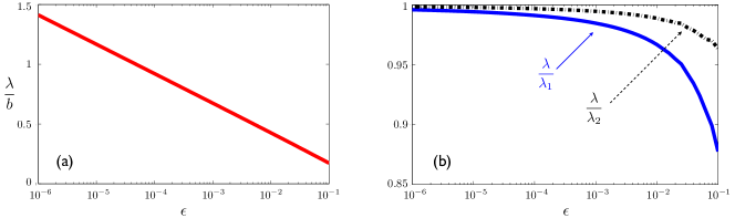
Figure 4: (color online) (a): Dimensionless effective slip length for the mesh-like super-hydrophobic surface, $\lambda/b$, as a function of the aspect ratio of the mesh, $\epsilon$. (b): Ratio between the slip length given by solving Eqs. (26) and the simple estimates provided by Eq. (33) ($\lambda/\lambda_{1}$, blue, solid line) and Eq. (36) ($\lambda/\lambda_{2}$, black, dash-dotted line), as a function of the aspect ratio.

III.1 Numerical results

We now solve numerically the infinite series given by Eqs. (26) by truncating it at a finite value $m_{1}=m_{2}=N$. The numerical results are displayed in Fig. 4a, where we plot the dimensionless slip length, $\lambda/b$, as a function of the aspect ratio of the mesh, $\epsilon$, for a truncation size of $N=10^{2}$. The exact size of the truncation has little influence on the final computed results; for example, when $\epsilon=10^{-3}$, the relative change in the computed slip length is less than 0.01 % between $N=10^{2}$ and $N=10^{3}$.

Our results show that the surface does show a reduction in friction (i.e. $\lambda>0$), and the effective slip length, always on the order of (but typically smaller than) the mesh size, increases when the solid area fraction decreases. Since the data on Fig. 4a are plotted on a semilog scale, we see that we recover the expected logarithmic relationship between the effective slip length of the mesh and its aspect ratio philip72 ; philip72_2 ; lauga03 ; ybert07 . A least squares fit to the data shown on Fig. 4a leads to the empirical formula

$${\frac{\lambda}{b}=\Lambda\ln{\epsilon}+\Pi,}$$ (31)

where the values $\Lambda=-0.107$ and $\Pi=-0.069$, gives result with maximum relative error of 0.4%. Alternatively, if we define the solid area fraction of the surface $\phi_{s}$, it is easy to see that $\phi_{s}=\epsilon(2-\epsilon)$. A least-square fit of the type

$$\frac{\lambda}{b}=\Lambda_{2}\ln{\phi_{s}}+\Pi_{2},$$ (32)

with the parameters $\Lambda_{2}=-0.107$ and $\Pi_{2}=0.003$, leads to a maximum relative error of $0.6\%$. As a matter of comparison, the fit proposed in Ref. ng09_2 , based on numerical simulations for $\phi_{s}\gtrsim 0.05$, leads to a relative error of 5% with the small-$\phi_{s}$ results obtained here; the asymptotic calculations presented in this paper are therefore able to quantitatively agree with the results of Ref. ng09_2 which are valid for much larger mesh sizes.

III.2 Comparison with simple estimates

An estimate of the mesh slip length can be obtained analytically by performing the truncation by hand. If only $A_{0},B_{0}$ — that is the mean values of the density functions with respect to $w$ — are retained in Eqs. (26), the surviving two equations give the lowest-order estimate

$$\frac{\lambda_{1}}{b}=\frac{1}{\pi(A_{0}+B_{0})}=\frac{1}{3\pi}\ln\left(\frac{2}{\pi\epsilon}\right)\cdot$$ (33)

We define here $L=\ln(2/\pi\epsilon)$ for subsequent convenience. Note that the slope of the relationship given by Eq. (33) is $1/3\pi\approx 0.106$, which is very close to the fitted value $|\Lambda|=0.107$ in Eq. (31).

Further, on writing Eqs. (26) and (26) as

$$3&=(A_{0}+B_{0})\ln\left(\frac{2}{\pi\epsilon}\right)+\sum_{m=1}^{\infty}\frac{(-1)^{m}}{m}(A_{m}+B_{m}),\\ -1=(A_{0}-B_{0})\ln\left(\frac{2}{\pi\epsilon}\right)-\sum_{m=1}^{\infty}\frac{(-1)^{m}}{m}(A_{m}-B_{m}),$$ (34)

and observing that the matrix elements in Eqs. (26) have $L$ only on the diagonal, it may be deduced that

$$\frac{\lambda_{1}}{b}-\frac{L}{3\pi}=O(L^{-1}).$$ (35)

As an illustration of this result, the truncation of Eqs. (26) at $m_{1}=m_{2}=1$ shows that the leading-order correction to Eq. (33) leads to the improved estimate

$$\frac{\lambda_{2}}{b}=\frac{L}{3\pi}-\frac{L+\frac{1}{2}}{6\pi\left[L^{2}+\frac{1}{4}L-\frac{1}{2}+\frac{9}{4\sqrt{2}}(L+\frac{1}{2})\right]}\cdot$$ (36)

On Fig. 4b, we show the ratio between the actual slip length (as calculated in Fig. 4a), and the simple estimates from Eq. (33) (blue, solid line) and Eq. (36) (black, dash-dotted line). We see that these simple formulae over-estimate the slip length (by up to 10%), but asymptotically converge to the correct result when $\epsilon\to 0$. As expected, the second-order solution, Eq. (36), is quantitatively better than the first-order one, Eq. (33).

IV Conclusion

In this work we have considered super-hydrophobic surface in the shape of a square mesh, and have presented an analytical method to calculate their effective slip length. Our analysis, which is valid for asymptotically small aspect ratio of the mesh, agrees also quantitatively with numerical calculations valid for larger mesh width ng09_2 . The results we obtain show that, for thin meshes, such surfaces can provide slip lengths on the order of the mesh size. However, for realistic mesh aspect ratio, say 10% or larger, the slip length is only a fraction of the typical mesh length (see Fig. 4). The increase of the slip length with the solid-to-air ratio of the overall surface is logarithmic, a universal feature of super-hydrophobic coatings with long and thin no-slip domains philip72 ; philip72_2 ; lauga03 ; ybert07 . Beyond such physical scaling, our results provide a first analytical prediction for the resistance to shear flow of the recently devised super-hydrophobic surfaces made of metal wires feng04 ; sun05 , and more generally to geometries with grid-like features such as fabric and textiles composed of interwoven threads.

Although we have considered here an idealized model system, the analytical approach developed in the paper has the advantage that it provides the effective slip length of the surface with relative error of order $\epsilon\log(1/\epsilon)$, which is significantly better than the more traditional but only logarithmically correct slender-body approach.

References

- (1) H. A. Stone, A. D. Stroock, and A. Ajdari. Engineering flows in small devices: Microfluidics toward a lab-on-a-chip. Annu. Rev. Fluid Mech., 36:381–411, 2004.
- (2) T. M. Squires and S. R. Quake. Microfluidics: fluid physics on the nanoliter scale. Rev. Mod. Phys., 77:977–1026, 2005.
- (3) L. Feng, S. H. Li, Y. S. Li, H. J. Li, L. J. Zhang, J. Zhai, Y. L. Song, B. Q. Liu, L. Jiang, and D. B. Zhu. Super-hydrophobic surfaces: From natural to artificial. Adv. Materials, 14:1857–1860, 2002.
- (4) D. Quere. Non-sticking drops. Rep. Prog. Phys., 68:2495–2532, 2005.
- (5) T. L. Sun, L. Feng, X. F. Gao, and L. Jiang. Bioinspired surfaces with special wettability. Acc. Chem. Res., 38:644–652, 2005.
- (6) D. Quere. Wetting and roughness. Annu. Rev. Fluid Mech., 38:71–99, 2008.
- (7) C. Neto, D. R. Evans, E. Bonaccurso, H.-J. Butt, and V. S. J. Craig. Boundary slip in newtonian liquids: A review of experimental studies. Rep. Prog. Phys., 68:2859–2897, 2005.
- (8) E. Lauga, M. P. Brenner, and H. A. Stone. Microfluidics: The no-slip boundary condition. In A. Yarin C. Tropea and J. F. Foss, editors, Handbook of Experimental Fluid Dynamics. Springer, New-York, 2007.
- (9) L. Bocquet and J.-L. Barrat. Flow boundary conditions: From nano- to micro-scales. Soft Matter, 3:685–693, 2007.
- (10) J. Ou, B. Perot, and J. P. Rothstein. Laminar drag reduction in microchannels using ultrahydrophobic surfaces. Phys. Fluids, 16:4635–4643, 2004.
- (11) J. Ou and J. P. Rothstein. Drag reduction and -PIV measurements of the flow past ultrahydrophobic surfaces. Phys. Fluids, 17:103606, 2005.
- (12) S. Gogte, P. Vorobieff, R. Truesdell, A. Mammoli, F. van Swol, P. Shah, and C. J. Brinker. Effective slip on textured superhydrophobic surfaces. Phys. Fluids, 17:051701, 2005.
- (13) C. H. Choi, U. Ulmanella, J. Kim, C. M. Ho, and C. J. Kim. Effective slip and friction reduction in nanograted superhydrophobic microchannels. Phys. Fluids, 18:087105, 2006.
- (14) R. Truesdell, A. Mammoli, P. Vorobieff, F. van Swol, and C. J. Brinker. Drag reduction on a patterned superhydrophobic surface. Phys. Rev. Lett., 97:044504, 2006.
- (15) D. Maynes, K. Jeffs, B. Woolford, and B. W. Webb. Laminar flow in a microchannel with hydrophobic surface patterned microribs oriented parallel to the flow direction. Phys. Fluids, 19:093603, 2007.
- (16) C. Lee, C. H. Choi, and C. J. Kim. Structured surfaces for a giant liquid slip. Phys. Rev. Lett., 101:064501, 2008.
- (17) J. R. Philip. Flows satisfying mixed no-slip and no-shear conditions. Z. Angew. Math. Phys., 23:353–372, 1972.
- (18) J. R. Philip. Integral properties of flows satisfying mixed no-slip and no-shear conditions. Z. Angew. Math. Phys., 23:960–968, 1972.
- (19) E. Lauga and H. A. Stone. Effective slip in pressure-driven Stokes flow. J. Fluid Mech., 489:55–77, 2003.
- (20) C. Cottin-Bizonne, C. Barentin, E. Charlaix, L. Bocquet, and J. L. Barrat. Dynamics of simple liquids at heterogeneous surfaces: Molecular-dynamics simulations and hydrodynamic description. European Phys. J. E, 15:427–438, 2004.
- (21) J. Davies, D. Maynes, B. W. Webb, and B. Woolford. Laminar flow in a microchannel with superhydrophobic walls exhibiting transverse ribs. Phys. Fluids, 18:087110, 2006.
- (22) C. Ybert, C. Barentin, C. Cottin-Bizonne, P. Joseph, and L. Bocquet. Achieving large slip with superhydrophobic surfaces: Scaling laws for generic geometries. Phys. Fluids, 19:123601, 2007.
- (23) C.-O. Ng and C. Y. Wang. Stokes shear flow over a grating: Implications for superhydrophobic slip. Phys. Fluids, 21:013602, 2009.
- (24) C. H. Choi and C. J. Kim. Large slip of aqueous liquid flow over a nanoengineered superhydrophobic surface. Phys. Rev. Lett., 96:066001, 2006.
- (25) P. Joseph, C. Cottin-Bizonne, J. M. Benoit, C. Ybert, C. Journet, P. Tabeling, and L. Bocquet. Slippage of water past superhydrophobic carbon nanotube forests in microchannels. Phys. Rev. Lett., 97:156104, 2006.
- (26) C.-O. Ng and C. Y. Wang. Apparent slip arising from Stokes shear flow over a bidimensional patterned surface. Microfluid. and Nanofluid., In Press, 2009.
- (27) A. Steinberger, C. Cottin-Bizonne, P. Kleimann, and E. Charlaix. High friction on a bubble mattress. Nature Mat., 6:665–668, 2007.
- (28) J. Hyvaluoma and J. Harting. Slip flow over structured surfaces with entrapped microbubbles. Phys. Rev. Lett., 100(24):246001, 2008.
- (29) D. Legendre and C. Colin. Enhancement of wall-friction by fixed cap-bubbles. Phys. Fluids, 20:051704, 2008.
- (30) A. M. J. Davis and E. Lauga. Geometric transition in friction for flow over a bubble mattress. Phys. Fluids, 21:011701, 2009.
- (31) L. Feng, Z. Y. Zhang, Z. H. Mai, Y. M. Ma, B. Q. Liu, L. Jiang, and D. B. Zhu. A super-hydrophobic and super-oleophilic coating mesh film for the separation of oil and water. Angew. Chem. Int. Ed., 43:2012–2014, 2004.
- (32) S. T. Wang, Y. L. Song, and L. Jiang. Microscale and nanoscale hierarchical structured mesh films with superhydrophobic and superoleophilic properties induced by long-chain fatty acids. Nanotech., 18:015103, 2007.
- (33) J. Happel and H. Brenner. Low Reynolds Number Hydrodynamics. Prentice Hall, Englewood Cliffs, NJ, 1965.
- (34) S. Kim and J. S. Karrila. Microhydrodynamics: Principles and Selected Applications. Butterworth-Heinemann, Boston, MA, 1991.
- (35) F.G. Leppington and H. Levine. Some axially symmetric potential problems. Proc. Edinburgh Math.Soc., 18:55–76, 1972.
- (36) R.P. Roger and R.G. Hussey. Stokes drag on a flat annular ring. Phys. Fluids, 25:915–922, 1982.
- (37) K. Stewartson. On mass flux through a torus in stokes flow. ZAMP, 34:567–574, 1983.
- (38) A.M.J. Davis and D.F. James. Slow flow through a model fibrous porous medium. Int. J. Multiph. Flow, 22:969–989, 1996.
- (39) A.M.J. Davis. A hydrodynamic model of the oscillating screen viscometer. Phys. Fluids, A5:2095–2103, 1993.
- (40) H. Hasimoto. On the periodic fundamental solutions of the stokes equations and their application to viscous flow past a cubic array of spheres. J. Fluid Mech., 5:317–328, 1959.